Global optimisation based control algorithms applied to boundary layer transition problems

Control Engineering Practice 12 (2004) 475–490

Global optimisation-based control algorithms applied to boundary

layer transition problems

G.V. Veres

, O.R. Tutty

, E. Rogers

*, P.A. Nelson

a_{School of Engineering Sciences, University of Southampton, Southampton SO17 1BJ, UK} b_{Department of Electronics and Computer Science, University of Southampton, Southampton SO17 1BJ, UK}

c_{Institute of Sound and Vibration Research, University of Southampton, Southampton SO17 1BJ, UK}

Received 27 January 2003; received in revised form 29 September 2003; accepted 30 September 2003

Abstract

Turbulent flow has a significantly higher drag than the corresponding laminar flow at the same flow conditions. The presence of turbulent flow over a large part of an aircraft therefore incurs a significant penalty of increased fuel consumption due to the extra thrust required. One possible way of decreasing the drag is to apply surface suction to delay the transition from laminar to turbulent flow. However, in order for the gain from the reduction in drag to outweigh the extra costs associated with the suction system, the suction must be distributed in an optimum, or near optimum, manner. In this paper two practical cases are considered. In the first of these a flat plate with panels whose positions are adjustable but do not overlap is treated. Since the cost function in this case is multi-modal, non-smooth and non-convex, methods for solving the optimisation problems necessary to design multi-panel suction systems based on direct search techniques are developed. In the second case considered the problem is that of linear distributed suction over the front part of an aerofoil. For this case, the computational load increases so significantly that in some cases it is not really feasible to continue the investigation using a single processor code. To overcome this, three parallel global optimisation algorithms are developed for the design of multi-panel suction systems on an aerofoil and it is shown that good solutions can be found efficiently.

r2003 Elsevier Ltd. All rights reserved.

Keywords: Boundary layer transition control; Flow control; Aerofoils; Non-smooth direct optimisation; Parallel global optimisation

1. Introduction

In recent years a number of ways have been considered for drag reduction and hence reduced operating costs for civil aircraft due to a decrease in

the fuel consumption (seeThiede (2001)for a summary

of some recent work in this area). It is well established that suction applied to surface of a body can delay the onset of transition from laminar to turbulent flow and thereby reduce the overall drag. Consequently, surface suction is regarded as one of the most promising methods for drag reduction. However, in order to maximise the benefit from the applied suction, it is necessary to distribute the suction in an optimum, or near optimum, way.

In the current work, the approach consists, in effect, of monitoring the state of the flow together with the

automatic control of suction applied through the surface of the body. This program involves both algorithm development and verification and wind tunnel based experiments. In the case of the latter, an essential element has been the development of techniques for monitoring the position of transition in a boundary layer. Experimentally, pressure measurements are used to determine the position of transition, and a control law is then used to maintain transition at a desired location with minimum power consumption by control-ling the suction flow rates on suction panels.

Previous work has demonstrated that this overall strategy is technically feasible both in simulation studies (of which computational fluid dynamics is an essential part) (Tutty, Hackenberg, & Nelson, 2000a, b) and by

wind tunnel-based experiments (Nelson, Wright, &

Rioual, 1997; Wright & Nelson, 1999). This work

employed gradient-based controllers, which used a local linear model constructed by standard linear system identification tools around selected operating points. For the case of flow over a flat plate these controllers *Corresponding author. Tel.: 592197; fax:

+44-2380-594498.

E-mail address:[email protected] (E. Rogers).

performed well. In somewhat more complicated cases, however, they did not, e.g. when a non-zero pressure gradient is applied to a flat plate (Tutty et al., 2000b).

InMacCormack, Tutty, Rogers, and Nelson (2002)it

was shown that the gradient-based approach failed when it was incompatible with the basic physics of the flow. An alternative approach, based on the use of Simulated Annealing and Genetic Algorithm methods to solve a non-linear optimisation problem, was

presented inDodd, Tutty, and Rogers (2001),

MacCor-mack et al. (2002). However, although this approach

was successful, computationally it is very demanding (and hence the time taken to obtain a satisfactory design may be (in relative terms) too long).

This paper first reports new results on the develop-ment of optimisation-based approaches for solving the design problem for the generic case of flow past a flat plate where the positions of the panels are calculated during the optimisation process, which for ease of terminology here we will term ‘moving panels’. The key point here is to include the panel positions as parameters in the optimisation task and hence obtain their best possible locations for minimising the cost function. This is a major advance on the previous work where we were optimising the suction flow rates for pre-positioned panels. A second new problem treated here is for an airfoil as opposed to panels where the computational cost will be (in relative terms) higher and the amount of time needed to complete the necessary design run may well be excessive (again in relative terms). Hence we also develop parallel versions of the algorithms for this case. There is no claim that the proposed methods are always preferable to all other methods (in particular, the development of parallel algorithms should not be read as implying that the computations cannot be done sequentially but merely that they may release a designers time for other tasks). Rather, the choice of optimisation technique to be used will be determined by the demands of the application problem or/and the preferences of user (but this, of course, requires a range of algorithms with known properties to be available). Note however that the speed of the algorithm is a critical feature if such methods are to be incorporated into a design process with practical constraints, when it may be necessary to repeat the calculation many times. The optimisation of the suction distribution under fixed flow conditions is a problem of considerable practical significance as this reflects cruise conditions for transport aircraft.

In the next section, we give the necessary background results. To provide context and a validated test case, the following section gives a description and some typical results from experiments performed for a flat plate with two suction panels. This is followed by a description of the models, cost functions, and algorithms used in this work. Representative results are given and discussed. Previous work (Tutty et al., 2000a, b) has shown that the

models developed below can be used to formulate a problem whose solution has good qualitative agreement with those from the experiments, including the dynamic behaviour under a control law.

2. Background

Consider a flat plate with a sharp leading edge aligned with a uniform incoming flow. Over most of the flow field, the effect of the viscosity of the fluid is negligible, and the flow will remain uniform. However, near the plate, the velocity must decrease from the free stream velocity to zero at the surface of the plate, and in this region, the ‘boundary layer’, viscous effects play a significant role. The width of the boundary layer is small compared with the length of the plate, but it increases along the plate, asx1=2_{;wherexis the distance along the}

plate from the leading edge, with the gradient of the velocity decreasing asx1=2_:

Suppose now that small disturbances are introduced into the flow in the boundary layer. Near the leading edge, forxox0;where

x0E6104n=UN ð1Þ

andUNandnare the free stream velocity and kinematic

viscosity of the fluid, respectively, these disturbances decay in amplitude, and the flow is stable. However, for

x>x0 the disturbances will grow, and the flow is

unstable. These disturbances, known as Tollmien– Schlichting waves, initially grow relatively slowly, but further downstream will provoke much more vigorous disturbances which rapidly lead to transition and a fully turbulent flow.

One of the primary characteristics of turbulent flow is enhanced mixing due to the rotational character of the small scale motions in the flow. In particular, in a turbulent boundary layer, the turbulence transports momentum from (the higher mean velocity) outer flow towards the wall and increases the velocity near the wall compared to that found in a laminar (non-turbulent) flow in similar conditions. This increases the velocity gradient at the wall, and since the shear stress (the frictional force) is proportional to the velocity gradient, the shear stress increases drastically, by at least an order of magnitude, at transition.

This paper is concerned with practical methods of delaying transition. There are a number of ways this can be achieved. For example, heating the surface will heat the fluid adjacent to it, and increase its kinematic viscosity, and enhance the stability of the flow: from (1)

it can be seen that increasing n will move the point at

which the flow becomes unstable downstream. However, in the aerospace industry there is a great deal of interest in using suction to delay transition. It has long been known that, in theory, withdrawing very small amounts of fluid from the boundary layer through the wall can greatly enhance the stability characteristics of the flow. In practice, suction flow rates are at least an order of magnitude greater than those suggested by the basic theory for a flat plate. However they are still small, and suction is regarded as one of the most viable means for practical drag reduction.

This paper considers distributed suction using discrete suction panels of the type commonly used in the aerospace field, but with the ability to vary the suction flow rate on each panel independently to optimise the effort required to achieve a desired objective. Different objectives and hence cost functions may be specified in different situations. For an aerofoil the aim will not be to simply delay transition as much as possible, but also to minimise the energy consumption of the system taking account of a number of factors. On a nacelle however, the design requirement is to fix transition at a particular point so that the benefits of laminar flow are obtained ahead of this point but the flow at the trailing edge of the nacelle is turbulent. Turbulence is desirable at the trailing edge of a nacelle as the contribution to the total drag from the pressure rather than the skin friction is substantially decreased in a body with a large blunt trailing edge if the flow is turbulent in this region. Both of these design requirements will be considered below.

Note that the transition scenario outlined above, through the amplification of linear Tollmien–Schlichting waves is not the only way that transition can occur. In particular, in a ‘noisy’ environment, a ‘bypass’ mechan-ism may operate where this linear stage may be absent completely, and transition may occur much more rapidly. However, in an environment with a low free stream turbulence level, there should be a relatively long region in which this linear mechanism is important, and where surface suction as considered in this paper can have a significant effect on the flow.

3. Experimental configuration

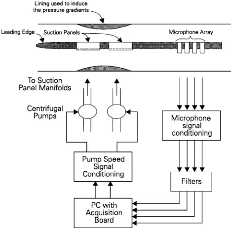
A simple experimental arrangement, for which an extensive series of tests has been performed (see e.g.

Nelson et al., 1997) is shown inFig. 1. A flat plate with,

if required, a smooth 2D hump on the wall opposite to

generate a pressure gradient, and two suction panels, one upstream and one downstream of the peak of the hump, is positioned in a wind tunnel with mean flow

speeds up to 22 m=s: The suction panels are made of

laser drilled titanium sheets, which provides a surface which is sufficiently smooth so as not to provoke transition through surface roughness. The holes have a

diameter of 0:1 mm (approximately), and are randomly

distributed with a density of 106_{holes per square metre,}

giving a porosity (hole area to surface area) of around

0.78%. Suction flow rates of up to 2 cm=s are possible,

where the suction flow rate is defined as the volume flow per unit surface area, and hence the flow in the holes is of the order of the suction flow rate divided by the porosity.

The humps are circular arcs 0:36 m long with a radius

of 0:555 m; giving a blockage of 10.3%. The suction

panels are located such that, according to hot wire anemometry experiments, without suction transition occurs on the second panel. Each suction panel is connected to a pump which is controlled by a PC via an inverter. Downstream of the two panels an array of flush-mounted microphones is installed. There were

eight microphones, positioned from 0.77 to 0:885 m

from the leading edge. This covers the range of possible transition positions for the conditions in this wind tunnel. The signals of these microphones are high pass filtered at 800 Hz in order to remove the background noise due to the wind tunnel fan. The microphone signals are sampled at a sampling rate of 4 kHz for a given period, then the rms value is calculated. These rms values are then normalised by pre-measured rms values of the signals for a fully turbulent boundary layer, hence

yielding a value close to 0 for laminar flow and a value close to 1 for turbulent flow.

The location of the laminar-turbulent transition is determined by comparison of the rms pressures acquired by the microphones to four reference pressures. The resulting error signal can be described by

eðkÞ ¼X

4

m¼1

½prefðxmÞ pðxm;kÞ

¼X

4

m¼1

prefðxmÞ X4

m¼1

pðxm;kÞ ¼ryðkÞ; ð2Þ

wherekis the iteration index,ris the sum of the desired

normalised pressures, and yðkÞ is the sum of the

measured normalised pressures. The desired normalised pressures are produced when transition is in the specified location. For the experimentsrandyðkÞare referred to as the desired plant output and the actual plant output, respectively. These two values are also directly related to

the desired transition location d and the actual

transition locationxT;such that (1) is equivalent to

eðkÞp½dx_TðkÞ: ð3Þ

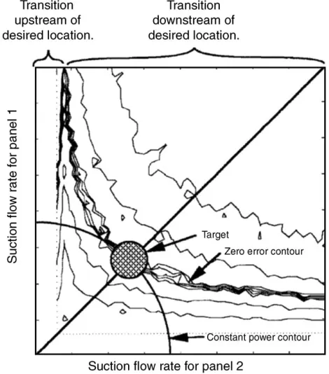
As illustrated in Fig. 2, an appropriate choice of the

reference pressures enables the specification of the location of the transition region with respect to the

microphone positions.Fig. 3shows, for a constant mean

flow speed, the position of transition as a function of the suction flow rates on the two panels. The contour lines indicate the position of transition.Fig. 3also illustrates the purpose of the controller which will regulate the two suction flow rates in this case until the shaded point is reached. This point corresponds to zero error with the minimum possible suction effort.

Further details of this experimental work and the

apparatus can be found inRioual (1994).

4. Theoretical modelling

When simulating viscous laminar flow it is possible to solve the full governing equations, the Navier–Stokes

equations, numerically. However, with the type of high Reynolds numbers considered here it is more efficient to apply Prandtl’s theory which assumes that the viscous part of the flow is restricted to a thin boundary layer, and solve a reduced set of equations which contain all the essential physics of the problem. The viscous part of the flow is described by the normalised boundary-layer equations:

*

u@u*

@x*þv*

@u*

@y*¼u*e

du*e

dx* þ

@2_u*

@y*2; ð4Þ

@u*

@x*þ

@v*

@y*¼0 ð5Þ

with the following boundary and initial conditions:

*

y¼0: u*¼0; v*¼v*wall; ð6Þ

*

y-N: u*ðx*;y*Þ-u*_eðx*Þ; ð7Þ

*

x¼x*0: Blasius profile; ð8Þ

whereu*andv*are the axial and the transverse velocities,

*

ueis the axial velocity at the edge of the boundary layer,

andx*andy*are the streamwise and normal coordinates. The variables in (4)–(8) have been non-dimensionalised using the scalings

*

u¼ u

UN

; v*¼ v

UN

ffiffiffiffi

R

p

; x*¼x

L; y*¼ y L

ffiffiffiffi

R

p ;

Normalised rms pressure

x x_{1 2 3 4}x x x

Microphone positions Transition upstream

of desired location

Transition at desired location

of desired location Transition downstream 1

Fig. 2. Monitoring the transition position using surface mounted microphones.

whereUNis the free-stream velocity,Lis the length of

the plate, R¼rUNL=m is the free stream Reynolds

number,ris the density, andmthe viscosity of the fluid.

The edge velocity u*e in (7) comes from a first-order

potential flow calculation for the flow past the body. A standard finite difference method is used to solve (4)–(8). In this work it is assumed that the transition from laminar to turbulent flow is preceded by the linear amplification of small 2D travelling waves, the so-called Tollmien–Schlichting waves. Note that this is only one possible scenario for transition to turbulence, and that there are other, much more vigorous, mechanisms that can cause transition resulting in bypass transition (see

e.g.Schmid & Henningson (2001) for discussion of this

and other relevant details). However, the assumption of linear amplification of small disturbances, and transition prediction through the growth of these disturbance (the

eN _{method—see below), forms part of a standard}

method used in the aerospace industry for the design of wings, fins and nacelles, and will therefore be employed here.

Linear hydrodynamic stability theory describes the stability of the flow to this kind of disturbance. A detailed description of the linear stability theory is given,

for example, by Mack (1977, 1984), therefore only the

main features are discussed in this paper. Linear stability theory is based on the study of small perturbations super-imposed on a basic laminar flow. The purpose of this theory is to determine the conditions under which these perturbations are amplified or damped. Therefore the velocity components and the pressure are decom-posed into an undisturbed mean part and a small disturbance. This decomposition is introduced into the unsteady 2D Navier–Stokes equations. The resulting equations are simplified by making the approximation

that the products of disturbance quantities are

negligible.

The result of the above analysis is a set of linear disturbance equations. The pressure is then eliminated by cross-differentiation. In the resulting equation the disturbance is expressed as a normal mode:

jðx;y;tÞ ¼FðyÞeiðaxotÞ; ð9Þ

where j is the (dimensionless) disturbance stream

function, a is the wave number, othe wave frequency

of the disturbance, and F is the (complex) disturbance

amplitude. This leads to the following disturbance velocities:

#

u¼F0eiðaxotÞ; ð10Þ

#

v¼ iaFeiðaxotÞ_{; ð11Þ}

where the prime stands for differentiation with respect

to y: Introducing these velocities into the disturbance

equation yields

uo

a

ðF00a2_{FÞ u}00_F

þ i

aReðF

0000_2a2_F00_þa4_{FÞ ¼0 ð12Þ}

the well known Orr–Sommerfeld equation. The

Rey-nolds numberRe is now based on the local

boundary-layer thickness, and u is the streamwise component of

the mean-flow velocity, obtained by the solution of the boundary-layer equations. Note that there is an implicit re-scaling here between the variables used for the flow calculation and the stability calculation.

Eq. (12) defines an eigenvalue problem with

homo-geneous boundary conditions (u# and v# must vanish at

the wall and in the free stream). For a given Reynolds number and real frequency, the solution yields an eigenfunction in the form of the complex disturbance amplitude and as an eigenvalue, the complex wave

number a¼arþiai: The imaginary part of the wave

number, ai gives the spatial growth rate of the

dis-turbance, which is positive for damped waves and negative for amplified waves. The speed of propagation of the disturbance is given byar=o:

Using linear stability theory, the onset of instability can be predicted, but instability is only a very early precursor of ultimate transition to turbulent flow. The

eN_{-method is a standard approach to relating the point}

of transition to the amplification of the disturbance waves. The total amplification rate is calculated by

integrating the spatial amplification factors ai at each

single real frequencyo:

ln A

A0

¼

Z x

x0

aidx; ð13Þ

whereAis the wave amplitude and the index 0 refers to

the streamwise position where this wave becomes unstable.

The eN_{-method is based on the envelope of these}

curves of total amplification, whereN is the maximum

amplification factor at each point:

N¼max ln A

A0

: ð14Þ

The position of transition is then predicted as the first

point at whichNexceeds a critical valueNT which can

vary according to the operating conditions of the flow.

Malik (1990)gives an extensive overview over the values

of NT found in various wind tunnel and flight

experiments. For a low free-stream turbulence level,

NT ¼10 proves to be a reasonable approximation.

However, Mack (1977, 1984) shows that this critical

amplification factor is strongly dependent on the turbulence level, and suggested the following relation:

where the turbulence level is calculated as

Tu¼

ffiffiffiffiffiffiffiffiffiffiffiffiffiffiffiffiffiffiffiffiffiffiffiffiffiffiffiffi

u02_þv02_þw02

3

s

with ðu0_;v0_;w0_{Þ denoting the dimensionless turbulent}

disturbance velocities and the overline averaging with

respect to time. In the present case the value of NT is

determined by comparison with the experiments of

Nelson et al. (1997). This givesNT ¼4:3;corresponding

to a free-stream turbulence level of approximately 0.5%. The calculations reported below use air at standard conditions, with kinematic viscosity of 1:5105 _m2_=s;

and a free stream velocity of 20 m=s:All lengths will be

in metres and velocities in m=s;and where convenient

these units will be dropped.

5. Cost functions

One relatively simple cost function for this general problem area is obtained by fixing the transition position at a pre-determined location, and then mini-mising the effort by varying the suction flow rates and the positions of the panels to achieve the best result. This is clearly of practical interest as it comes directly from the design requirements for a suction control system on a nacelle. We formulate two (slightly) different optimisation problems for the two scenarios we consider in this paper: flow past a flat plate where the position of the panels are not fixed but are adjusted as part of the optimisation procedure (moving panels) and flow past an aerofoil with fixed panels and linearly distributed suction flow rates. The first of these scenarios reflects the fact that the minimum effort depends on not just the amount of suction, but also its distribution. The second, is a generalised version of a suction system consisting of a relatively large number of contiguous plenum chambers under the front part of the body providing a near continuous suction distribution. Both are based on systems of practical interest and have not been the subject of any detailed investigation in the literature to-date.

Note here that a transition location is some function of suction flow rates and there is an unknown or, at best, very complicated relationship linking the panel positions and flow rates, i.e. essentially ‘black box’ optimisation problems have to be treated here. Also there clearly must be bounds on the suction flow rates and here it is assumed that these are known.

5.1. Cost function for moving panels on a flat plate

The problem of constraining the transition position to some desired location by finding optimal locations for the suction panels on flat plate can be formulated

as follows: Find optimal ðui;piÞ; i¼1yN; which minimise

f_s¼k1 XN

i¼1

u2_i; ð16Þ

subject to

xtxd ¼0:

Here ui denotes the suction flow rate through panel i

which runs from x¼pi to x¼piþH;where pi is the

starting point of panel i and the panels are of equal

lengthH;f_sis an estimate of the suction effort,Nis the

number of panels, k1 is a positive constant, ui is the

suction flow rate through panel i; xt is the current

transition position as predicted using the methods

described in the previous section, andxd is the desired

transition position. A key point here is that panels are not fixed, and their position is found as part of the solution to the problem. There is however a further constraint in that the panels cannot overlap, and this limits the acceptable values of the pi still further. This

constrained minimisation problem can be rewritten as unconstrained minimum by solving the following problem:

Find optimalðui;piÞ;i¼1yN;which minimise:

f¼f_sþk2jxtxdjh; ð17Þ

wherek2is a positive constant, andhis a positive integer

to be selected based on knowledge of the specific

configuration being considered (here the case of h¼1

is treated). This last optimisation problem is nonlinear and, as experiments have shown, multi-modal. This is

true even for the case withN¼2;which is investigated

here numerically (Section 8) as a representative case. Note thatf_sis not a true measure of the suction effort, but it is a monotonic function of the power used by the

suction system, and hence minimisingf_s will produce a

valid solution.

The solution of the optimisation problem just defined is a two stage process. First we compute the optimal flow rates under (17) for a fixed non-overlapped pair of

ðp1;p2Þ of starting positions and then find optimal

positions of the two panels. Each of the stages is detailed in Sections 6.1 and 6.2. For optimisation purposes, it is assumed that there are known bounds on the positions of the panels.

5.2. Cost function for linearly distributed suction flow rates on an aerofoil

rates linearly distributed over panels a practically relevant cost function is of the form:

minimisef_s¼k1 X

Nþ1

i¼1

u2_i; ð18Þ

subject to xtxd ¼0: Here fs denotes the suction

effort by panel i; N is the number of panels, k1 is a

positive constant, ui is a suction flow rate at the

beginning of paneli;or the end of paneliifi¼Nþ1;

xt is the transition position and xd is the desired

transition position. Note that the suction flow rate at the beginning of paneliis equal to a suction flow rate at the

end of panel i1 for 1oioNþ1:As in the previous

problem, the constrained version can be rewritten as an unconstrained problem which here is of the form:

minimisef¼f_sþk2jxtxdjh; ð19Þ

where k2 is a positive constant, and h is as in the

previous case. Again this is a nonlinear problem and has been shown in experiments to be multi-modal.

To obtain a realistic problem in the case of an aerofoil, for example, can often require the number of

panels N to be very large and thereby lead to an

enormous computational burden. (Experiments have shown that it can take days to complete a design run.) Hence we develop and demonstrate the effectiveness of parallel algorithms for these problems. In this paper, the calculations are performed for an NACA 0012

aerofoil, with a chord of 1 m: In the numerical work

here (Section 9) the representative cases of 5 and 10 panels are considered.

6. Optimisation algorithms

In this and the next section we detail in turn the algorithms developed for use in the work reported in this paper.

6.1. Optimisation of the flow rates with fixed panels

Consider a case when two panels are used and are in fixed positions and the design objective is to compute suction flow rates which minimise a cost function of form (17). This cost function is nonlinear, non-differential and multi-modal. Moreover, evaluation of the objective function requires the running of expensive analysis codes.

Since the cost function is non-smooth, non-convex, non-differential and multi-modal, appropriately mod-ified versions of direct search methods are (potentially) the most appropriate here. Direct search methods of the form considered here have their origins in the work of

Nelder and Mead (1965) but it is later modifications

which are of particular interest. These are the so-called

deformed configuration methods (Rykov, 1995) and the

multi-directional search methods of Torczon (1991)

(which can also be regarded as members of the deformed configuration class of methods). Here we will use an assortment of configuration types, i.e. a simplex, defined

to have c¼nþ1 vertices in n-dimensional space, a

complex, defined to cX_nþ_{2 vertices in n-dimensional}

space, of regular or irregular geometry, mapping functions, local optimality criteria, adaptation proce-dures and the rules for combining them, which together generate a class of deformed configuration methods. The major differences between the algorithm developed here

from those ofTorczon (1991)andRykov (1995)are an

additional preliminary procedure, the use of complex

vertices defined byc¼3n_{1 vertices in n-dimensional}

space, and the use of so-called accepted mapping directions to ensure that the global optimum of the multi-modal cost function is found.

Next we detail the so-called modified complex algorithm developed here for solving the optimisation problem under consideration. (In the numerical exam-ples of Sections 8.1 and 8.2, only the case of two panels will be considered.) This algorithm consists of three stages—initialisation, exploratory moves and the mod-ified direct search algorithm, respectively, which are now detailed in turn, and the cost function is denoted byFðÞ:

* _{Initialisation: Feasible bounds are defined and an}

inscribed complex is constructed within these bounds. The geometrical centre of the complex is calculated and the cost function values at the vertices of the complex and its centre are obtained through simula-tion.

* _{Exploratory moves: The purpose of these is to reduce}

the complex size and to attempt to locate the most likely regions for a global minimum. A line connected to each vertex of the complex and the complex centre is then divided into 10 intervals and cost function values obtained at these intervals. The point with minimum cost function value is taken as a new complex point, located in the direction of the old complex point and centre. After this operation a new complex with the same geometrical centre as the old one is constructed for further optimisation.

* _{Modified direct search algorithm: The basic operation}

of this algorithm is that a complex with c¼3n₁

vertices exists at each iteration. Then the geometrical centre of complex, together with the cost function values in each complex vertex and complex centre are obtained, and the correct enumeration of complex vertices is undertaken, i.e. such that the following chain of inequalities holds

Fðuðk;1ÞÞXFðuðk;2ÞÞX?XFðuðk;cÞÞ;

where k denotes the iteration number, and u is a

the vertices with cost function values greater than the cost function value at the centre of the complex are mapped through the geometrical centre of non-mapped vertices. If the cost function of a reflected vertex is less than that for the complex centre, the step-size is increased and a vertex of the new complex is taken to be one with the minimum cost function value, otherwise the original vertex is brought near to the complex centre. These iterations are repeated until either the stopping rule is satisfied or a pre-specified maximum number of iterations has been undertaken. The stopping rule used in this case is that the algorithm is assumed to have converged if

Fðuðk;1ÞÞ Fðuðk;cÞÞoe1

and

max

2oiocjju

ðk;1Þ_uðk;iÞ_jjoe 2

hold, where e1 and e2 are user specified convergence

measures (in the numerical work here both were set at 106).

The modified direct search algorithm can now be detailed as follows.

Initial Data to be specified—an initial complex

uð0;iÞ; i¼1;y;c(in the case of two panelsc¼8), the centre of the initial complexuðkÞ;the step-parameters

a; b; and g (here a¼1:9; b¼0:25; g¼1:1); the

maximum number of stepsNN (hereNN¼50)

for k¼0;1;yNN do

perform correct enumeration check the stopping rule

m’0

for i¼1;y;c do

if Fðuðk;iÞÞ>FðuðkÞÞ then

m’mþ1

for i¼1;y_;m do sðk;iÞðmÞ ¼ 1

cm

Pc

j¼mþ1 uðk;jÞ

uðkr;iÞ¼sðk;iÞðmÞ þgðsðk;iÞðmÞ uðk;iÞÞ calculateFðuðkr;iÞÞ

if Fðuðkr;iÞÞoFðuðkÞÞ then

uðke;iÞ ¼sðk;iÞðmÞ þaðsðk;iÞðmÞ uðk;iÞÞ calculateFðuðke;iÞÞ

if Fðuðke;iÞÞoFðuðkr;iÞÞ then uðkþ1;iÞ¼uðke;iÞ

Fðuðkþ1;iÞ_{Þ ¼Fðu}ðke;iÞ_Þ

else

uðkþ1;iÞ_¼uðkr;iÞ

Fðuðkþ1;iÞ_{Þ ¼Fðu}ðkr;iÞ_Þ

else

uðkþ1;iÞ ¼uðkÞbðuðkÞuðk;iÞÞ calculateFðuðkþ1;iÞÞ

for i¼mþ1;y;c do

uðkþ1;iÞ ¼uðk;iÞ;Fðuðkþ1;iÞÞ ¼Fðuðk;iÞÞ calculate new complex centreuðkþ1Þ andFðuðkþ1ÞÞ

The vertex which yields the minimum value of FðuÞ is

assumed to be the estimate of the minimum point.

Before proceeding further it should be noted that when the position of the panels is variable, different positions can result in different minimum values of the cost function.

6.2. Computing the optimal positions for two panels

When the positions of the panels (i.e.pi) are allowed

to vary, the complexity of the optimisation problem is considerably increased. Consider, however, the case of two panels. Then careful investigation of the final cost function shows that optimisation of the panel positions can be done independently of each other, i.e. fix one panel position whilst optimising the position of the other. Further, in this case the sub-cost function associated with the variable panel position is a unimodal 1D function. Hence the use of the golden section search method is proposed for the optimisation of each of

panel position, i.e. first p1 is chosen according to the

golden section method and then the same method is run

for p2: This approach is faster than going through all

possible combinations of panel positions and it

also enables either a global minimum or, at worst, a near optimal solution to be computed. Details of the golden search method are omitted here since it can be found in many optimisation textbooks (see, for example,

Fletcher, 1987).

Actual results (see Section 8) confirm that this algorithm can deliver good results but a major draw-back is that its complexity will grow exponentially with dimension, i.e. with the number of panels used. More-over, if the more realistic scenarios are considered (for example, continuous suction distributions over the front part of body with a realistic pressure gradient, etc.) and/ or more panels are used, a much larger computational effort would be required. To reduce computational time in such cases, a parallel version of the algorithm detailed above has been developed and investigated for a case of linearly distributed flow rates on an aerofoil as detailed next.

7. Parallel global optimisation of linearly distributed flow rates on an aerofoil

nonlinear, non-differential, multi-modal and where it is required to run expensive analysis codes. (The analysis and results given here start from the preliminary

findings in Veres, Tutty, Rogers, & Nelson, 2003b).

We consider three different classes of algorithms and also combinations of them. We now detail each of these in turn.

7.1. Random search method

These methods directly aim to find the global

minimum (Horst & Pardalos, 1995) and the version of

them used here consists of the following steps.

* _{Choose the initial number of pointsN}

1and set initial

feasible bounds on the flow rates.

* _{Select N}

1 uniformly distributed points within the

initial feasible bounds.

* _{Obtain the cost function values at the initial set of}

points concurrently and save the point with the minimum cost function value as the closest possible to an optimal solution.

* _{Taking into consideration cost function values,}

reduce the feasible bounds to areas more likely to contain optimal points and choose a number of

pointsN2 to be used within these new bounds.

* _SelectN

2uniformly distributed points within the new

feasible bounds and evaluate the cost functions at these points concurrently.

* _{Choose the point with the minimum cost function}

value from these new points and set the old near optimal solution equal to the new near optimal solution.

This approach can assist in refining the bounds on suction flow rates, but will require the use of a sufficient number of points to find the optimal or near optimal solution, i.e. to achieve a good coverage of the feasible region.

7.2. Parallel global optimisation method

Since the cost function (19) to be optimised is non-smooth, non-convex and multi-modal, we have already argued the case for the development of modifications of direct search methods to find the global minimum. Further support for these is provided by the fact that, for example, an asynchronous parallel pattern search

(Kolda, Hough, & Torczon, 2001), was successfully

implemented on parallel computing platforms for minimisation of objective functions which are expensive to evaluate.

Here we propose to use an algorithm which is one of a number of possible modifications of the deformed

configuration methods (Rykov, 1995), which belong to

the general class of direct search methods. In the method of deformed configurations, the basic feature of

constructing the simplex and applying an optimisation procedure to the complex is augmented by introducing search control. This consists of choosing the locally optimal direction, mapping the configuration vertices, the centroid, and the step-size, and leads to reduced cost function values. Also, since we are mapping several configuration (simplex or complex) vertices the number of which is automatically adjusted from step to step, these methods have relatively fast convergence and are less sensitive to noise corruption than the computation of the cost function at any instant.

The major differences between the algorithm pro-posed here and an asynchronous parallel pattern search

(Kolda et al., 2001) or the deformed configuration

methods (Rykov, 1995) are the addition of the

preliminary procedure and the (sophisticated) choice of mapping directions to ensure that we obtain the global optimum of multi-modal cost function. All the vertices are divided into three groups, i.e. mapped, reflected and the best vertex between best vertex of the complex and the complex centre. Mapped vertices are those whose cost function values are greater than the cost function value in the complex centre. Reflected vertices are those whose cost function values are less than or equal to those of the complex centre but also greater than cost function value at the best complex vertex, i.e. the complex vertex with the minimum cost function value in the complex.

After division of vertices the construction of a new complex is carried out as detailed below. All complex vertices are used here in the exploration of possible search directions and this gives better coverage of space in comparison to the original algorithm. This is a very important feature when there are several local optimum in the example under consideration.

In detail, the new algorithm for minimising the (19)

consists of three steps—initialisation, exploratory

moves, and the modified procedure for executing deformed configurations. These are described in turn next.

7.2.1. Initialisation

* _{Define feasible bounds for the suction flow rates.}

* _{Define the step-size parametersa;b;andg:}

* _{Select stopping tolerancestol}

1 andtol2:

* _{Select the maximum number of iterations N}

1 and

maximum number of iterations allowed without

changes in the minimum cost function valuesN2:

* _{Construct an inscribed complex u}ð0;iÞ_{; i¼1;y;c}

within the bounds and compute the geometrical centre of the complexuðkÞ:

* _{Evaluate the cost function values at the vertices}

7.2.2. Exploratory moves

(a) Divide a line connecting each vertex of the complex and the complex centre into ten intervals.

(b) Calculate the cost function values at the points defined in the last step concurrently.

(c) Take the point with minimum cost function value as a new complex point in the direction of the old complex point and centre.

7.2.3. Modified method of deformed configurations

1. If kpN1; then set k¼kþ1 (k is the iteration

counter) and go to Step 2. Else, exit.

2. Perform correct enumeration of complex vertices, i.e. such that the following chain of inequalities holds:

Fðuðk;1ÞÞXFðuðk;2ÞÞX?XFðuðk;cÞÞ:

3. If

ðFðuðk;1ÞÞ Fðuðk;cÞÞ_oe1

and

max

2oiocjju

ðk;1Þ_uðk;iÞ_jjo

e2Þ

or the number of iterations without the minimum cost function value changing is greater thanN2;exit.

Else, go to Step 4.

4. Divide all vertices into three groups: m mapped

vertices with Fðuðk;iÞÞ>FðuðkÞÞ; i¼1;y_{;m; q} re-flected vertices withFðuðk;iÞÞpFðuðkÞÞ andFðuðk;iÞÞ>

Fðuðk;cÞÞ; i¼1;y;q; q here is the vertex with the minimum cost function value from the set whose elements are the best complex vertices and the complex centre.

5. Map m vertices through the centre of unmapped

vertices

sðk;iÞðmÞ ¼ 1

cm

Xc

j¼mþ1

uðk;jÞ

according to

uðkr;iÞ¼sðk;iÞðmÞ þgðsðk;iÞðmÞ uðk;iÞÞ:

6. Reflect q vertices through the best complex

ver-tex with the minimum cost function value according to

uðkr;iÞ¼uðk;cÞþgðuðk;cÞuðk;iÞÞ:

7. If Fðuðk;cÞ_Þ>FðuðkÞ_{Þ; then reflect the best complex}

vertex through the complex centre

uðkr;cÞ ¼uðkÞþgðuðkÞuðk;cÞÞ:

Else, reflect the complex centre through the best complex vertex

uðkr;cÞ¼uðk;cÞþgðuðk;cÞuðkÞÞ:

8. Evaluate Fðuðkr;iÞÞ; i¼1;y;c;concurrently. 9. If Fðuðkr;iÞÞoFðuðkÞÞ; i¼1;y;m; then repeat the

mapping with a bigger step-size parameter a: Else,

repeat the mapping with a smaller step-size para-meterb:

10. If Fðuðkr;iÞÞoFðuðk;cÞÞ; i¼1;y;q; then repeat the

reflection with a bigger step-size parametera:Else,

repeat the reflection with a smaller step-size para-meterb:

11. If a reflected vertex in group q has a smaller cost

function value than a non-reflected vertex, repeat

the reflection with a bigger step-size parameter a:

Else, repeat the reflection with a smaller step-size parameterb:

12. Calculate cost function values at the newcvertices

concurrently.

13. Compare the cost function values computed for the

old set of c vertices with those at the new set of

corresponding 2c vertices obtained by reflection/

mapping with different step-size parameters.

Choose cvertices with the minimum cost function

values as the set of new complex vertices.

14. Calculate a new geometrical centre of the new complex and the cost function value in it.

The vertex which gives the minimum value of FðuÞ is

taken as the estimation of the minimum point.

In the above algorithm, parallelisation occurs only at the stage of computing the cost function values. Further parallelisation is, however, possible at the stage when the new complex vertices are being computed. Our experience has shown that this algorithm can find the

global optimum quite accurately (Veres, Tutty, Rogers,

& Nelson, 2003a), but the complexity of this problem

will grow exponentially with dimension and in case of 10 panels it requires weeks of computational time even on parallel processors to achieve either the global minimum or a ‘reasonable’ estimate of it.

These last facts have led to the development of the multi-start parallel global optimisation algorithm de-tailed next for higher dimensions where, crucially, the problem complexity will grow linearly rather than exponentially.

7.3. Multi-start parallel global optimisation

To speed up the optimisation process for a large number of panels, we have developed the following algorithm which, in effect, combines the multi-start parallel global optimisation algorithm with the pattern

search approach (Torczon, 1991) for local search tasks.

the local search starts and then apply this to selected points. Again, the resulting algorithm consists of three stages—initialisation, multi-start points selection, and local search which are detailed in turn next.

7.3.1. Initialisation

* _{Define feasible bounds for linear distributed flow}

rates.

* _{Define the step-size parametersa;b;andg:}

* _{Select the maximum number of iterations N}

1 and

maximum number of iterations allowed N2 without

changes in the minimum cost function value.

* _{Choose a number of complex verticescfor the local}

search.

* _{SelectNuniformly distributed random pointsu}

i; i¼

1;y_{;N;within the feasible bounds—these points will} form the set of initial pointsS0:

* _{Evaluate the values of the cost functions Fðu}

iÞ

concurrently.

7.3.2. Multi-start points selection

(a) Sort all points in ascending order with respect to the cost function values, i.e.u1anduNwill be the points

with minimum and maximum cost function values, respectively.

(b) Normalise all cost function values as

FnðuiÞ ¼

FðuiÞ Fðu1Þ

FðuNÞ Fðu1Þ

; i¼1;y;N:

(c) Remove the points from the setS0withFnðuiÞ>tol1:

(d) Do the following until there are no points left in set

S0:

(e) Add the first point to the set of multi-start pointsS:

(f) Calculate the Euclidean distances from this point to all other points, normalise these distances, and then

remove from the set Spoints with distances less or

equal to the chosen threshold tol2:Go to (d).

7.3.3. Local search

1. Letumin be a point with the minimum cost function

valueFðuminÞfrom the set S:

2. Choose the number of complex verticesc:

3. For each multi-start point in the set S do the

following.

4. Construct an initial complex. 5. min’argimin0pipc1Fðuð0;iÞÞ:

6. Swapuð0;minÞ anduð0;0Þ:

7. Ifk1pN1 and k2pN2;thenk1 ¼k1þ1 (k1 is—(as

before) the iteration number andk2is the number of

iterations for which there is no change in the minimum cost function value), go to Step 8. Else, go to Step 14.

8. Reflectc1 vertices through the best vertexuðk;minÞ

according to

uðkr;iÞ ¼uðk;minÞþgðuðk;minÞuðk;iÞÞ;¼1;y;c1:

9. Evaluate Fðuðkr;iÞÞ; i¼1;y_{;c1 concurrently.} 10. If Fðuðkr;iÞÞoFðuðk;minÞÞ; then repeat the mapping

with a bigger step-size parametera:Else, repeat the

mapping with a smaller step-size parameter b:

11. Evaluate the cost function values at the new c1

vertices concurrently.

12. Choose c1 vertices from the old vertices and

reflect them with different step-size parameters from the ones used to obtain the minimum cost function value.

13. If there is no change in the minimum cost function value setk2¼k2þ1;elsek2¼0:

14. The vertex uk;min _{with minimum value of FðuÞ is}

taken as the estimation of the minimum point. 15. If Fðuk;minÞ_oFðuminÞ; replace umin by uk;min; and

FðuminÞbyFðuk;minÞ:Go to Step 3.

This algorithm is faster than the parallel global optimisation algorithm based on the deformed config-uration method, but its accuracy will be depend on the thresholds in the multi-start points selection stage and on the number of vertices in the initial complex for each multi-start point. To obtain a compromise between accuracy and the speed of global optimisation, a combination of a random search procedure and a multi-start parallel global optimisation is proposed below.

7.4. Combination of random search procedure and multi-start parallel global optimisation

If the most important criterion is accuracy, then it is possible to combine the random search method with multi-start parallel global optimisation. The idea here is simple—initial (ideally wide ranging) bounds for flow rates are defined and then a random search is used to narrow these bounds to regions more likely to contain the global optimum. Following this, the multi-start parallel global optimisation is applied with these new bounds in place. The steps in implementing this algorithm can be summarised as follows.

* _{Choose an initial number of points N}

1 and initial

feasible bounds for the flow rates.

* _{Select N}

1 points uniformly distributed within the

initial feasible bounds.

* _{Compute the cost function values for the initial set of}

points concurrently.

* _{Based on cost function values, reduce the feasible}

* _{SelectNuniformly distributed random pointsu}

i; i¼

1;y;N;from within the feasible bounds, where these points will form the set of initial pointsS0:

* _{Evaluate the cost function valuesFðu}

iÞconcurrently.

* _{Perform multi-start points selection and the local}

search stages of the multi-start parallel global optimisation algorithm with the initial bounds for flow rates.

Note here that after choosing multi-start points, the bounds on flow rates are relaxed again. The purpose of this is to avoid missing the global minimum. (Since only a ‘coarse’ investigation of regions containing global solutions is undertaken (to avoid having an excessive number of points to evaluate), there is the possibility that a global minimum will be outside, but very close to, the reduced bounds.)

8. Results: optimisation of the flow rates with two moving panels

Consider a flat panel 1 m long with 2 non-overlapping suction panels, where the lengths of the panels are both

equal to 0:1 m with a minimum gap of 0:05 m between

them. To reduce the computational burden, the follow-ing bounds were imposed on the positions of the panels:

p1A½0:18;0:55; p₂A½p₁þ0:15;0:7: The desired

transi-tion is taken as xd ¼0:8 m and also the following cost

function parameters (see alsoMacCormack et al., 2002)

were used k1¼104;k2¼10 andh¼1:

8.1. Optimisation of the flow rates with fixed panels

To check the robustness of this algorithm the following actions were taken. First, the simulations were run without optimisation and the desired transition

point was achieved by changing the panel positions in

steps of 0:01 m; subject to the constraint that they

cannot overlap. The required suction flow rates were determined as follows. First, an initial guess of possible

suction flow rates was made and then transition pointxt

was computed by a suitable computational fluid dynamics (CFD) code for given flow rates. If the

difference between desired transition point xd and

calculated transition point xt was greater than a

specified tolerance, the flow rates were adjusted using:

uiðkþ1Þ ¼uiðkÞ 0:001ðxdxtÞ;

where i¼1;y;N (k is the iteration index). This

procedure was then repeated until either convergence occurred or the maximum allowed number of iterations had been completed. Note also that in this case that flow rate will be the same for each panel.

The minimum cost function value achieved with the above approach is given inTable 1, where in this and all other tables in this paper, distances are given in metres, flow rates in metres per second, and the cost functions involved have been non-dimensionalised by suitable choices of units for the constantsk1 andk2:

Now with fixed panels positionsðp1;p2Þ ¼ ð0:27;0:51Þ

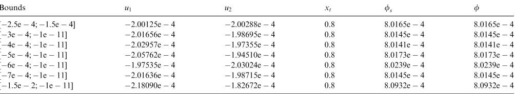
the optimisation algorithm was applied. Different initial bounds were used to judge algorithm convergence from different starting regions. The results are given in

Table 2. As can be seen from Table 2, applying the

optimisation algorithm does reduce the overall cost,

primarily by movingxt closer to xd;but in some cases

reducing the suction cost by a small amount as well.

Note also that the results in Table 2 were all obtained

with the same values of the tuning parametersa;bandg:

We also found that the suction cost can be further reduced, but not to any significant extent, by varying the parametersa;bandg:The running time of the algorithm for fixed panel positions depends on initial bounds and

Table 1

The minimum overall cost function without optimisation but with moving panels

p1 p2 u1 u2 xt fs f

0.27 0.51 2:002e4 2:002e4 0.799968 8:0160e4 8:3360e4

Table 2

The minimum overall cost function with optimisation and fixed panel locationsð0:27;0:51Þ

Bounds u1 u2 xt fs f

½2:5e4;1:5e4 2:00125e4 2:00288e4 0.8 8:0165e4 8:0165e4

½3e4;1e11 2:01656e4 1:98695e4 0.8 8:0145e4 8:0145e4

½4e4;1e11 2:02957e4 1:97355e4 0.8 8:0141e4 8:0141e4

½5e4;1e11 2:05762e4 1:94510e4 0.8 8:0173e4 8:0173e4

½6e4;1e11 1:97535e4 2:03024e4 0.8 8:0239e4 8:0239e4

½7e4;1e11 2:01636e4 1:98715e4 0.8 8:0145e4 8:0145e4

did not exceed 2 h for a chosen set of bounds on a 500 MHz PIII processor.

8.2. Finding the optimal positions of two panels

For this task, we first need to know where the actual global minimum located as this will allow us to estimate how good our optimisation actually is. For this purpose, the positions of the panels were changed by increments

of 0:01 m and optimisation was applied for each

non-overlapping pair ðp1;p2Þ: Table 3 gives the resulting

global minimum solution (for this set-up).

Clearly this way of finding the global minimum is very heavy computationally and is useful only for compar-ison purposes. The results of applying the golden section search algorithm together with modified complex

optimisation are given in Table 4 (where after each

calculation the panel positions were rounded up to two

digits after decimal point). The results in Table 4 are

identical to those inTable 3, but the computational load is reduced.

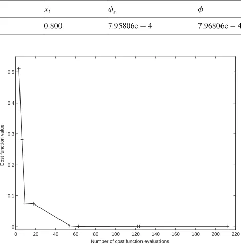
Fig. 4 shows the variation of the cost function with

the iteration count. Clearly, a good if not optimum solution is found relatively quickly, with further, slow, refinement later in the run. Similar plots were obtained in all other cases and are omitted here for brevity.

9. Results: linear distributed suction flow rates on an aerofoil

In this section the different methods developed in Section 7 are compared for the representative cases of 5 and 10 non-overlapping panels fixed at 20% of the chord with linear continuous suction flow rate distribu-tions for 2D flow. In particular, the three solution algorithms developed in Sections 7.2, 7.3 and 7.4 respectively above are compared with the random search

approach (Section 7.1). The parametersa;bandgwere

set at 1.9, 0.29, and 1.1, respectively, throughout these comparisons, and the thresholds tol1¼0:15 and tol2¼

0:5 were set for multi-start points selection. Initial

feasible sets for the flow rates were taken to be in the range½3:7e4;0:

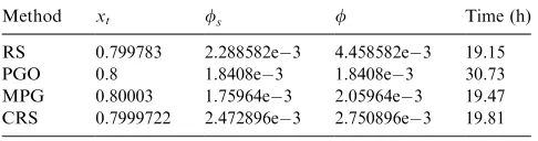
9.1. 5 panels case

Here random search (RS), parallel global optimisa-tion based on the modified deformed configuraoptimisa-tion method (PGO), multi-start parallel global optimisation with pattern search for local search (MPG), and a combination of random search and multi-start parallel

global optimisation (CRS) are compared. For RS,N1¼

8190 and N2¼3567 were chosen. Also the set S0

contained 2900 initial points, and the setScontained 10

multi-start points for MPG. In the case of CRS,N1¼

3567; S0 contained 2900 points and S contained 13

multi-start points. The results obtained are given in

Tables 5 and 6. Note thatu1has been set to zero in this

work since immediate vicinity of the leading edge of the aerofoil, where this suction effort would be applied, the flow is accelerating and stable to disturbances of the type considered here.

In Table 6, it is the elapsed rather than the total

computational time which is given, where the former is Table 3

Global minimum solution when optimisation is applied and the panels are moving

p1 p2 u1 u2 xt fs f

0.27 0.48 1:995460e4 1:994041e4 0.800 7:95806e4 7:95806e4

Table 4

The optimal solution when both the golden section search method and modified complex method are applied

p1 p2 u1 u2 xt fs f

0.27 0.48 1:99546e4 1:994041e4 0.800 7:95806e4 7:96806e4

0 20 40 60 80 100 120 140 160 180 200 220 0

0.1 0.2 0.3 0.4 0.5

Number of cost function evaluations

Cost function value

much larger due to the parallel structure of the solution method. The number of processors used varied, and was adjusted to suit the problem and make best use of the resources available, by ‘load balancing’ the processor array so that there was very little idle time. For example, in the RS case, 22 processors where used for the first

stage of the (N1¼8190—1 master processor and 21

workers) and 30 for the second stageðN2¼3567Þ;while

for CRS 15, 15 and 4 processors were used for the three stages, respectively.

As can be seen from theTable 6, PGO provides the

best solution, but also requires almost twice as much time to obtain a solution compared to the RS, MPG and CRS methods. Moreover the complexity of PGO method, and execution time required as result of this, grows exponentially with increasing optimisation pro-blem dimension. The MPG method suggests itself as a good compromise between accuracy and computational load, and in comparison CRS method is worse in both these respects. However, the performance of these two algorithms depend on the tuning parameters, the type of problem considered and the dimension of the resulting optimisation problem. Finally, it is to be expected that the CRS method will out-perform the MPG approach in terms of accuracy.

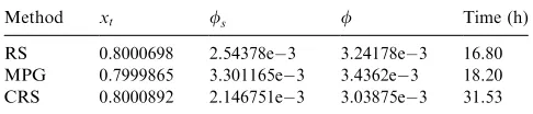
9.2. 10 panels case

Here the RS, MPG and the CRS methods are compared for a case with 10 panels. The reason why PGO is not included that it is too slow for 11D optimisation problem which has to be solved in this

case. For RS N1¼8190 and N2¼8961 were chosen.

The set S0 contained 9984 initial points, and the setS

contained 13 multi-start points for MPG. In the case of

CRS N1¼8190;the setS0 contained 9984 points, and

the setS contained 20 multi-start points.

The results of the comparison are given inTables 7–9,

respectively. It can be seen from Table 9 that CRS

method produces the best solution, as expected. How-ever, it requires the longest computational time and hence the preferences of users or/and the type of the application problems considered will decide which one of the proposed methods to choose for use for the underlying global optimisation problem. Note also that, since all three methods have a degree of randomness associated with them, it is not guaranteed that the results will be the same if we start from different initial data sets. This is most relevant for the RS since the other two attempt to find the global or near optimal minimum.

The values given in Table 9 for the cost function

values are larger than those given inTable 6for the case of 5 panels. This is deceptive in that the cost function takes no account of the length of the panels. To obtain a

direct comparison, the values in Table 9 should be

divided by two. This shows that shorter panels produce solutions with lower total suction effort, as would be expected on physical grounds.

10. Conclusions

Turbulent flow has a significantly higher drag than the corresponding laminar flow at the same flow conditions. The presence of turbulent flow over a large part of an aircraft therefore incurs a significant penalty of in-creased fuel consumption due to the extra thrust required. One possible way of decreasing the drag is to apply surface suction to delay the transition from laminar to turbulent flow. However, in order for the gain from the reduction in drag to outweigh the extra costs associated with the suction system, the suction must be distributed in an optimum, or near optimum, manner. The results presented here show that the modified complex method developed in this paper applied with a golden section search method can be used to optimise the panel positions and suction distribution for a two panel system. Although this approach is relatively efficient, there is still a trade off between finding the optimal solution and the computa-tional load. However, it is clear that if the aim is to find a ‘good’ solution, i.e. one that is close to the optimal Table 5

The near optimal flow rates for 5 panels

Method u1 u2 u3 u4 u5 u6

RS 0 6.66254e5 3.444661e4 3.134907e04 8.161225e5 2.872861e5

PGO 0 1.5e5 1.1e5 9.0e5 3.6999e4 1.9683e4

MPG 0 0 4.32388e5 0 3.67273e4 1.98027e4

CRS 0 1.580755e4 4.168359e5 9.0e5 3.442298e4 3.065454e4

Table 6

The minimum overall cost functions obtained for 5 panels

Method xt fs f Time (h)

RS 0.799783 2.288582e3 4.458582e3 19.15

PGO 0.8 1.8408e3 1.8408e3 30.73

solution with a significant reduction of the cost, rather than the optimal solution, then this can be done quickly. In case of an aerofoil with a linear continuous suction distribution over its front part, the computational load increases significantly, and in some cases it is not possible to continue the investigation using a single processor. Therefore several parallel global optimisation solution algorithms have been developed in this paper. For the representative case of 5 panels, the parallel global optimisation method based on modified de-formed configuration method (PGO) produced the best solution. However, this method requires 50% more computational time than random search method (RS) and multi-start parallel global optimisation method with pattern search for local search (MPG). Moreover, with an increase in dimensionality, the computational com-plexity of the PGO method will increase exponentially. Therefore for case of 10 panels we consider only RS, MPG and a combination of random search and multi-start parallel global optimisation (CRS). The results here showed that as expected CRS method gave the best solution in relative terms but it required more computa-tional time. Therefore there is still a trade off between finding the global minimum and the computational load and choice of the global optimisation approach will depend on preferences of user and/or an application problem considered.

Finally we note that the methods developed here have major advantages over those described in earlier work in that they can obtain solutions in cases where simpler gradient based methods fail (Tutty et al., 2000b) but are

much more efficient than methods based on stochastic

optimisation (Dodd et al., 2001; MacCormack et al.,

2002). Further, for the problems considered in

Mac-Cormack et al. (2002) which had a similar number of

variables to be determined as part of the solution, it was necessary to severely restrict the values the suction flow rates could take in order to obtain a relatively crude solution in a reasonable time.

References

Dodd, T. O. R., Tutty, & Rogers, E. (2001). Genetic algorithm based constrained optimisation for laminar flow control.Proceedings of the European control conference 2001(ECC’01), Porto, September 2001, pp. 2970–2974.

Fletcher, R. (1987). Practical methods of optimization. Chichester: Wiley.

Horst, R., & Pardalos, P. M. (Eds.). (1995). Handbook of global optimization. Dordrecht/Boston/London: Kluwer Academic Publishers.

Kolda, T. G., Hough, P. D., & Torczon, V. J. (2001). Asynchronous parallel pattern search for nonlinear optimization.SIAM Journal on Scientific Computing,23, 134–156.

MacCormack, W., Tutty, O. R., Rogers, E., & Nelson, P. A. (2002). Stochastic optimisation based control of boundary layer transition. Control Engineering Practice,10, 243–260.

Mack, L. M. (1977).Transition prediction and linear stability theory. AGARD CP-224, 1.1.

Mack, L. M. (1984).Boundary layer stability theory. AGARD Report 709, 3.1.

Malik, M. R. (1990). Stability theory for laminar flow control design. Progress in Aeronautics and Astronautics,123(3).

Nelder, J. A., & Mead, R. (1965). A simplex method for function minimization.The Computer Journal,7(4), 308–313.

Nelson, P. A., Wright, M. C. M., & Rioual, J.-L. (1997). Automatic control of laminar boundary-layer transition.AIAA Journal,35, 85–90.

Rioual, J.-L. (1994).The automatic control of boundary layer transition. Ph.D. thesis, University of Southampton.

Rykov, A. (1995). Construction principles of deformed configurations methods.Preprints of the summer school course on Identification and Optimization oriented for use in adaptive control, Prague, Czech Republic(pp. 65–80).

Table 8

The near optimal flow rates for 10 panels—cont’d

Method u7 u8 u9 u10 u11

RS 4:846197e5 1.02092e4 1.354573e4 3.570386e04 2.767380e4

MPG 3:352883e4 3.423307e4 0 7.614603e5 0

CRS 3:623112e4 2.624833ee4 0 0 0

Table 9

The minimum overall cost functions for 10 panels

Method xt fs f Time (h)

RS 0.8000698 2.54378e3 3.24178e3 16.80 MPG 0.7999865 3.301165e3 3.4362e3 18.20 CRS 0.8000892 2.146751e3 3.03875e3 31.53 Table 7

The near optimal flow rates for 10 panels

Method u1 u2 u3 u4 u5 u6

RS 0 4:517587e5 6.48977e5 6.626079e05 4:143352e5 8.269108e5

MPG 0 4:517458e5 8.147645e5 2.293512e4 1:702706e4 6.660711e5

Schmid, P. J., & Henningson, D. S. (2001).Stability and Transition in Shear Flows. New York: Springer.

Thiede, P. (Ed.). (2001). Aerodynamic Drag Reduction Technologies. Proceedings of the CEAS/DragNet European drag reduction Conference, Potsdam, Germany, June 2000. Berlin: Springer. Torczon, V. (1991). On the convergence of the multidirectional search

algorithm.SIAM Journal on Optimization,1(1), 123–145. Tutty, O. R., Hackenberg, P., & Nelson, P. A. (2000a). Numerical

optimisation of the suction distribution for laminar flow control. AIAA Journal,38, 370–372.

Tutty, O. R., Hackenberg, P., & Nelson, P. A. (2000b). Gradient projection based control and optimisation of the suction distribu-tion for laminar flow control. Proceedings of the Institution of

Mechanical Engineers Part I-Journal of Systems and Control Engineering,214, 347–359.

Veres, G. V., Tutty, O. R., Rogers, E., & Nelson, P. A. (2003a). On design optimisation based control methods for distributed suctions for boundary layer transition control. Proceedings of 2003 American control conference, Denver (pp. 2187–2192).

Veres, G. V., Tutty, O. R., Rogers, E., & Nelson, P. A. (2003b). Parallel global optimisation based control of boundary layer transition. 2003 European control conference, Cambridge, UK, CD-Rom proceedings.