City, University of London Institutional Repository
Citation:
Kaishev, V. K., Dimitrova, D. S., Haberman, S. and Verrall, R. J. (2006). Geometrically designed, variable know regression splines: asymptotics and inference (Statistical Research Paper No. 28). London, UK: Faculty of Actuarial Science & Insurance, City University London.This is the unspecified version of the paper.
This version of the publication may differ from the final published
version.
Permanent repository link:
http://openaccess.city.ac.uk/2372/Link to published version:
Statistical Research Paper No. 28Copyright and reuse: City Research Online aims to make research
outputs of City, University of London available to a wider audience.
Copyright and Moral Rights remain with the author(s) and/or copyright
holders. URLs from City Research Online may be freely distributed and
linked to.
City Research Online: http://openaccess.city.ac.uk/ [email protected]
Faculty of Actuarial
Science
and
Insurance
Geometrically Designed,
Variable Knot Regression
Splines: Asymptotics and
Inference.
Vladimir K. Kaishev, Dimitrina S. Dimitrova,
Steven Haberman and Richard Verrall.
Statistical
Research Paper No. 28
October 2006
ISBN 1-905752-02-4
Cass Business School
106 Bunhill Row
London EC1Y 8TZ
knot regression splines:
Asymptotics and inference
by
Vladimir K. Kaishev
*, Dimitrina S. Dimitrova, Steven Haberman
and Richard Verrall
Cass Business School, City University, London
Summary
A new method for Computer Aided Geometric Design of least squares (LS) splines with variable knots, named GeDS, is presented. It is based on the property that the spline regression function, viewed as a parametric curve, has a control polygon and, due to the shape preserving and convex hull properties, closely follows the shape of this control polygon. The latter has vertices, whose x-coordinates are certain knot averages, known as the Greville sites and whose y-coordinates are the regression coefficients. Thus, manipu-lation of the position of the control polygon and hence of the spline curve may be interpreted as estimation of its knots and coefficients. These geometric ideas are implemented in the two stages of the GeDS estima-tion method. In stage A, a linear LS spline fit to the data is constructed, and viewed as the initial posiestima-tion of the control polygon of a higher order (n>2 ) smooth spline curve. In stage B, the optimal set of knots of this higher order spline curve is found, so that its control polygon is as close to the initial polygon of stage A as possible and finally, the LS estimates of the regression coefficients of this curve are found. To implement stage A, an automatic adaptive knot location scheme for generating linear spline fits is developed. At each step of stage A, a knot is placed where a certain bias dominated measure is maximal. This stage is equipped with a novel stopping rule which serves as a model selector. The optimal knots defined in stage B ensure that the higher order spline curve is nearly a variation diminishing (i.e., shape preserving) spline approxima-tion to the linear fit of stage A. Error bounds for this approximaapproxima-tion are derived in Kaishev et al. (2006). The GeDS method produces simultaneously linear, quadratic, cubic (and possibly higher order) spline fits with one and the same number of B-spline regression functions.
Large sample properties of the GeDS estimator are also explored, and asymptotic normality is established. Asymptotic conditions on the rate of growth of the knots with the increase of the sample size, which ensure that the bias is of negligible magnitude compared to the variance of the GeD estimator, are given. Based on these results, pointwise asymptotic confidence intervals with GeDS are also constructed and shown to converge to the nominal coverage probability level for a reasonable number of knots and sample sizes.
Keywords: spline regression, B-splines, Greville abscissae, variable knot splines, control polygon, asymp-totic confidence interval, coverage probability, asympasymp-totic normality
1. Introduction.
Consider a response variable y and an independent variable x, taking values within an interval @a,bD and assume there is a relationship between x and y of the form
(1)
y= fHxL+ e,
where fHÿL is an unknown function and e is a random error variable with zero mean and variance Ee2= s2>0. We will consider the regression problem of estimating fHÿL, based on a sample of observations 8xi, yi<i=1
N . The design points 8x
i<iN=1 may be either
deterministic or random.
Different methods for the solution of this regression problem have been proposed and the related literature is extensive. One popular approach is to approximate f with an
n-th order (degree n-1) spline function defined on @a,bD. As is well known, n-th order splines, on a set of k internal knots, form a linear functional space, an element of which is represented as a linear combination of appropriate spline basis functions. Thus, a spline function is defined by its order n, by the number and location of its k internal knots and by the coefficients in front of the basis functions.
It is also well known that least squares fitting with splines of a fixed degree is a linear optimization problem, if the number of knots and their location are fixed. However, since the latter are in general unknown and need to be defined, several approaches to constructing free-knot regression splines have been developed. The direct approach is to assume that n and k are fixed (but unknown), and to find the knot locations which mini-mize the (non-linear) least squares criterion (see e.g. Jupp, 1978) or an appropriately penalized version of it (see Lindstrom, 1999). For an extensive discussion of the (dis)advantages of non-linear free-knot spline estimation, we refer to Lindstrom (1999).
In order to circumvent the difficulties related to the non-linear optimization approach, a number of authors have developed adaptive knot selection procedures, such as step-wise knot inclusion/deletion strategies. Among the latter are the early work of Smith (1982), the TURBO spline modelling technique of Friedman and Silverman (1989), the MARS method proposed by Friedman (1991), the POLYMARS of Stone et al. (1997) and the spatially adaptive regression splines (SARS) of Zhou and Shen (2001). Other methods, such as the knot removal algorithm of Lytch and Mørken (1993) and the minimum description length (MDL) regression splines of Lee (2000), have been proposed as well. Multivariate spline regression and knot location has also been considered by Kaishev (1984). Further references to alternative spline fitting methods, such as smoothing spline techniques are to be found in Kaishev et al. (2006).
knot placement density and the number of knots which minimize the asymptotic inte-grated mean square error. More recently, Zhou et al. (1998) and Huang (2003), have studied local (pointwise) asymptotic properties of least squares regression splines. Under the assumption of asymptotic uniformity of the knot placement, Zhou et al. (1998) provide explicit expressions for the asymptotic pointwise bias and variance of regression splines. A less stringent assumption on the knot mesh has been considered by Huang (2003), who establishes some asymptotic results for general estimation spaces. These asymptotic results shed some light on the large sample properties of least squares splines under some conditions on the joint asymptotic behaviour of the number and position of the knots and the sample size.
In this paper, we present a new variable knot spline regression estimation method which is very different from the existing methods and includes two stages. In stage A, a least squares linear spline regression fit to the data is constructed, following a novel knot location method. The latter places knots sequentially, one at a time, at sites where a certain bias dominated measure is maximal. Stage A is equipped with an appropriate stopping rule which serves as a model selector (see Section 3, and Appendix A for the complete description of stage A). In stage B, an optimal set of knots of a smoother, higher order Hn>2L least squares spline approximation is found so that the latter has also the characteristics of a Schoenberg's variation diminishing spline approximation of the linear spline fit from stage A. We show that this new spline regression estimation method has a direct Geometric Design interpretation. It stems from the fact that Schoen-berg's variation diminishing spline approximation scheme is the fundamental concept underlying parametric B-spline curve and surface modelling in Computer Aided Geomet-ric Design (see e.g. Farin, 2002). For this reason we will call our new method the GeD spline estimation method and will refer to the related estimator as a GeD spline estima-tor or simply GeDS. Optimality properties of the knots of the GeD spline estimaestima-tor are established in Kaishev et al. (2006) where further algorithmic details, related to GeDS, are also to be found. The numerical performance of GeDS, compared to other existing spline estimators is addressed more thoroughly in Kaishev et al. (2006). In the present paper, the focus of our attention is on introducing this new spline estimator and on its statistical properties. Under some mild conditions on the design points 8xi<iN=1, we
estab-lish its asymptotic normality and give conditions under which the bias term of the approx-imation error becomes asymptotically negligible compared to the variance term. The construction of pointwise asymptotic confidence intervals is also considered and illus-trated numerically.
coeffi-cients and knots, it is proposed that their estimation is performed through positioning the control polygon of the spline regression curve so that it follows the noise-perturbed shape of the underlying function. This geometric characterization of the regression problem is used in Section 3 to develop the GeD spline regression estimation method and in particular, to formulate its two stages, A and B, as optimization problems. In Section 4, some pointwise asymptotic properties of the GeDS estimator are established. The GeDS method and its properties are illustrated numerically in Section 5, based on a simulated example. It is shown how the large sample results of Section 4 can be used to construct asymptotic pointwise confidence intervals with a required coverage probabil-ity. In Section 6 we provide some discussion and conclusions. Detailed description of part A of GeDS are given in Appendix A and proofs of the results of Section 4 are given in Appendix B.
2. The B-spline regression and its control polygon.
Denote by Stk,n the linear space of all n-th order spline functions defined on a set of
non-decreasing knots tk,n=8ti<i2=n1+k, where tn=a, tn+k+1=b. In this paper we will use
splines with simple knots, except for the n left and right most knots which will be assumed coalescent, i.e., tk,n=8t1= ...=tn<tn+1<...<tn+k<tn+k+1= ...=t2n+k<. Following the Curry-Schoenberg theorem, a spline regression function f œStk,n, can be
expressed as
fHtk,n;xL=q'NnHxL=⁄i=1
p q
iNi,nHxL,
where q=Hq1, ...,qpL' is a vector of real valued regression coefficients and
NnHxL=HN1,nHxL, ..., Np,nHxLL', p= n+k, are B-splines of order n, defined on tk,n. It is well known that ⁄i=j-n+1
j
Ni,nHtL=1, for any tœ@tj,tj+1L, j=n, ...,n+k, and
Ni,nHtL=0 for t–@ti,ti+nD.
In the sequel, where necessary, we will emphasize the dependence of the spline fHtk,n;xL on q by using the alternative notation fHtk,n,q;xL.
The spline regression problem of Section 1 can now be more precisely stated as follows. For a fixed order of the spline n, given a sample of observations 8yi, xi<iN=1, estimate the
number of knots k, their locations tk,n and the regression coefficients, q.
In order to solve this estimation problem and develop the GeD spline estimator, our purpose in this section will be first to introduce an alternative way of expressing the spline regression fHtk,n, q;xL. Recall that the standard way is to consider it as a function of the independent variable xœ@a,bD, following the expression
fHtk,n,q;xL=⁄i=1
p q
(2)
QHtL=8xHtL, yHtL<=8⁄ip=1xiNi,nHtL,⁄i=1
p q
iNi,nHtL<,
where t is a parameter, and xHtL and yHtL are spline functions, defined on one and the same set of knots tk,n, with coefficients xi and qi, i=1, ..., p, respectively. If the coeffi-cients xi in (2) are chosen to be the knot averages
(3)
xi*=Ht
i+1+...+ti+n-1L ê Hn-1L, i=1, ..., p,
then it is possible to show that the identity
(4)
xHtL=⁄ip=1xi*Ni,nHtL=t ,
referred to as the linear precision property of B-splines, holds. In view of (2) and (4), the spline regression function fHtk,n,q;xL can be expressed as a parametric spline curve as
(5)
Q*HtL=8t, fHtk,n,q;tL<=8⁄i=1
p x
i*Ni,nHtL,⁄i=1
p q
iNi,nHtL< ,
where tœ@a,bD and xi* is the average of the n-1 consecutive knots ti+1, ...,ti+n-1
given by (3). In what follows, it will be convenient to use Q*HtL and fHtk,n,q;tL inter-changeably to denote a functional spline regression curve.
The values xi* given by (3) are known as the Greville abscissae. We will alternatively use the notation x*Htk,nL, to indicate the dependence of the set of Greville sites
x* =8x1*, ...,x
p
*<ªx*Ht
k,nL on the knots tk,n.
The interpretation (5) of the regression function fHtk,n,q;xL as a parametric spline curve
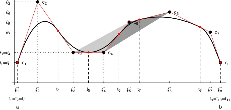
Q*HtL is fundamental for our aim of developing a geometrically motivated least squares, variable knot, spline regression smoother. It allows us to characterize the spline regres-sion curve Q*HtL by a polygon, which is closely related to Q*HtL, and is called the control polygon of Q*HtL, denoted by CQ*HtL. It is constructed by connecting the points
ci=Hxi*,qiL, i=1, ..., p, called control points, by straight lines. So, CQ*Hxi*L= qi,
i=1, ..., p. In Fig.1, the geometric relationship between a spline regression curve and its control polygon CQ*HtL is illustrated. This relationship is due to the fact that both the
x and y coordinates of the control points ci, i=1, ..., p, are related to the spline regres-sion curve Q*HtL. More precisely, the x-coordinates, xi*, are the Greville sites (3), obtained from the knots tk,n, and the y-coordinates, qi, are simply the spline regression coefficients. Since, ⁄ij=j-n+1Ni,nHtL=1, for any tœ@tj,tj+1L, j=n, ... , n+k, the curve
Q*HtL is a convex combination of its control points, and its graph lies within the convex hull of its control polygon CQ*. The convex hull of c1, ..., cp is the smallest convex
polygon, enclosing these points. Due to the convex hull property, the curve is in a close vicinity of its control polygon which is illustrated in Fig. 1 with respect to two adjacent polynomial segments of Q*HtL. The grey areas in Fig. 1 are the two convex hulls, formed by c3,c4,c5 and c4,c5,c6, within which the two segments of Q*HtL, for tœ@t5,t6D and
tœ@t6,t7D, lie. For further details related to geometric modelling with splines we refer to
x1*
t1=t2=t3
a
x2
* x
3
* x
4
* x
5
* x
6
* x
7
*
t4 t5 t6 t7 t8 x8*
t9=t10=t11
b
q1=q8
q2
q3=q4
q5
q6
q7
c1
c2
c3 c4
c5
c6
c7
[image:9.595.96.466.88.265.2]c8
Fig. 1. A quadratic, functional spline regression curve Q*HtL and its control polygon CQ*.
Another reason for the spline regression curve Q*HtL to be close to its control polygon
CQ*HtL is that Q*HtL is the Schoenberg's variation diminishing spline approximation of
CQ*HtL, i.e.,
(6)
V@CQ*DHtL=⁄i=1
p
CQ*Hxi*LNi,nHtL=⁄i=1
p q
iNi,nHtLªQ*HtL,
where xi*, i=1, 2, ..., p, are the Greville abscissae, obtained from tk,n and CQ*Hxi*L= qi by the definition of the control polygon.
Given a set of knots, tk,n, the spline approximation V@gDHxL=⁄i=1
p
gHxi*LNi,nHxL of any function g, defined on @a,bD, is known as the Schoenberg's variation diminishing spline (VDS) approximation of order n to g, on the set of knots tk,n. It is constructed by simply evaluating g at the Greville sites (3) and taking the values gHxi*L as the B-spline coeffi-cients of the VDS approximation.
It is important to recall a property of V@gD, which is crucial for developing the GeD estimator. That is, the VDS approximation, V@gD is shape preserving since it preserves the shape of the function g it approximates. More precisely, if g is positive, then V@gD is also positive, if g is monotone, then V@gD is also monotone, and if g is convex, V@gD is also convex. The variation diminishing character of V@gD is due to the fact that it crosses any straight line at most as many times as does the function g itself. In view of the convex hull property and the shape preserving property of (6) it is more clear why Q*HtL
lies so close to its control polygon CQ*HtL.
In summary, it has been established that the spline regression function fHtk,n,q;xL, (which we alternatively denoted as Q*HxL, xœ@a,bD), can be expressed in the form (5) and that its control polygon, CfHtk,n,q;xL, has vertices ci=Hxi
*,q
iL, i=1, ...p, where xi* are the Greville sites (3), obtained from tk,n. The latter suggests that, given n and k, locating the knots tk,n and finding the regression coefficients q of fHtk,n,q;xL, based on the set of observations 8yi, xi<iN=1, is equivalent to finding the location of the x- and y-coordinates
q affects the geometrical position of the control polygon CfHtk,n,q;xL, which, due to the
shape preserving and convex hull properties, defines the location of the spline curve
fHtk,n,q;xL. Inversely, locating the vertices ci of CfHtk,n,q;xL affects the knots tk,n, through
(3), and the values of q, and hence affects the position of the regression curve
fHtk,n,q;xL. The latter conclusion motivates the construction, in stage A of GeDS, of a control polygon as a linear least squares spline fit to the data, whose knots determine the knots tk,n, and whose B-spline coefficients are viewed as an initial estimate of q, which is improved further in stage B (see Section 3). This is the basis of our approach to con-structing the GeD variable knot spline approximation to the unknown function f in (1), and this is developed in the next section.
3. Geometrically designed spline regression.
In this section we introduce the GeD spline regression method which is motivated by the ideas, outlined in Section 2. The method "positions" first an initial control polygon, which reproduces the "shape" of the data, applying least squares approximation. Sec-ondly, an optimal set of knots of a higher order Hn>2L smooth spline curve is found, so that it preserves the shape of the initial control polygon and then this curve is fitted to the data, to adjust its position in the LS sense. In this way, it is ensured that the n-th order smooth LS fit follows the shape of the initial control polygon, and hence the shape of the data. This procedure simultaneously produces quadratic, cubic, or higher order splines and the LS fit with the minimum residual sum of squares is chosen as the final fit which recovers best the underlying unknown function f. The two stages of this approach may be given a formal interpretation as certain optimization problems with respect to the variables k,tk,n,q and n. Hence, the approach produces a solution which does not necessarily coincide with the globally optimal solution under the free-knot non-linear optimization approach. As illustrated by the numerical examples presented here and also in Kaishev et al. (2006), it produces LS spline fits which are characterized by a small number of non-coalescent knots and very low mean square errors. Thus, GeD spline fits are shown to be nearly optimal (see the example in Section 5 and also exam-ples 1 and 2 of Kaishev et al., 2006) and to enjoy some very good large sample proper-ties, such as asymptotic normality, established in Section 4. The latter allow for the construction of asymptotic confidence intervals illustrated in Section 5. The GeD spline estimation involves the following two stages:
Stage A. Fix the order n=2. Starting from a straight line fit and adding one knot at a time, find the least squares linear spline fit f`Hdl,2,a`;xL=⁄i=1
p a`
iNi,2HxL with a number
of internal knots l, number of B-splines p=l+2 and with a set of knots
dl,2=8d1= d2< d3<...< dl+2< dl+3= dl+4<, such that the ratio of the residual sums of
squares
RSSHl+qL êRSSHlL=‚
j=1
N
Hyj- f
`
Hdl+q,2;xjLL
2
í ‚Nj=1 Hyj- f
`
Hdl,2;xjLL
where aexit is a certain threshold level. This means that f
`
Hdl,2,a`;xL could not be
signifi-cantly improved if q more knots are added, q¥1, and therefore, f`Hdl,2,a`;xL adequately reproduces the "shape" of the unknown, underlying function f. The linear LS spline fit f`Hdl,2,a`;xL is viewed as a control polygon with vertices Hxi,a`iL, i=1, ..., p, where
xiª di+1, i=1, ..., p. The fit f
`
Hdl,2,a`;xL is constructed following an algorithm
described in Appendix A.
Stage B. For each of the values of n=3, ..., nmax, find the optimal position of the knots
t
é
l-Hn-2L,n, as a solution of the constrained minimization problem
(7) min
tl-Hn-2L,n,
xi+1<ti+n<xi+n-1,
i=1,...,k
±f`Hdl,2,a`;xL-CfHtl-Hn-2L,n,a`;xLµ¶,
where ∞g¥¶:=maxa§x§b » gHxL » defines the uniform (L¶) norm of a given function
gHxL, and xi, i=1, ..., p are the x-coordinates of the vertices of the control polygon f`Hdl,2,a`;xL obtained in stage A. In fact, minimization in (7) is over all polygons
CfHtl-Hn-2L,n,a`;xL with verticesHxi*,a`iL, whose x-coordinates coincide with the Greville sites
x*Htl-Hn-2L,nL, and whose y-coordinates, coincide with the y-coordinates a`i of the vertices of the polygon f`Hdl,2,a`;xL. Clearly, the two polygons f`Hdl,2,a`;xL and CfHtl-Hn-2L,n,a`;xL
have the same number of vertices p=l+2, since the number of internal knots in
tl-Hn-2L,n is l-Hn-2L.
As shown in Kaishev et al. (2006), the optimization problem (7) has no optimal solution such that the minimum in (7) is zero, i.e., for which CfHté
l-Hn-2L,n,a`;xLª f
`
Hdl,2,a`;xL. Instead,
the objective of stage B, (i.e. of the minimization in (7)) is to produce a set of optimal knots tél-Hn-2L,n, which ensures that f
`
Hdl,2,a`;xL becomes (nearly) the control polygon of
the spline regression function fHétl-Hn-2L,n,a`;xL, i.e., that CfHtél-Hn-2L,n,a`;xL> f
`
Hdl,2,a`;xL. In
this way, tél-Hn-2L,n is placed so that fHt
é
l-Hn-2L,n,a`;xL becomes (nearly) the Schoenberg's variation diminishing spline approximation of f`Hdl,2,a`;xL and hence, due to its convex hull and shape preserving properties (see Section 2), fHtél-Hn-2L,n,a`;xL lies very close to f`Hdl,2,a`;xL, and hence to the "shape" of the data for which the linear LS approximation
is f`Hdl,2,a`;xL (according to stage A). This is the fundamental concept of optimal knot
placement in GeDS. For a proof of the fact that fHtél-Hn-2L,n,a`;xL is nearly a VDS approxi-mation of f`Hdl,2,a`;xL with appropriate error bounds, we refer to Kaishev et al. (2006)
(see Theorem 1 and Corollaries 1.1 and 1.2).
However, we note that the fit fHtél-Hn-2L,n,a`;xL will not be a least squares approximation to the data set. In order to obtain an LS fit to the data and at the same time to preserve the shape of fHtél-Hn-2L,n,a`;xL, its optimal knots t
é
l-Hn-2L,n are preserved, whereas its B-spline coefficients a`i are released and are assumed to be unknown parameters, q, which are estimated in the least squares sense, using 8yi, xi<iN=1. Thus, for a fixed
n=3, ...,nmax, we find the least squares fit f
`
Itél-Hn-2L,n,q
`
min
q A‚j=1
N
Hyj- fHt
é
l-Hn-2L,n,q;xjLL
2
E.
Finally, we choose the order nè whose fit f`Itél-Hnè-2L,nè,q
`
;xM has the minimum residual sum of squares. In this way, along with the number of knots and their locations, the degree of the spline is also estimated. This is an important feature of the proposed estimation method which is rarely offered by other spline estimation procedures. One alternative that we are aware of is the MDL method of Lee (2000). Of course, any of the produced final fits of order n∫nè could be used, if other features were more desirable, for example if better smoothness were required.
Since (7) is a constrained non-linear optimization problem, and although for linear splines, our experience shows that it is still difficult to solve. As with other nonlinear optimization problems, finding the global optimum is not guaranteed. The knots
t
é
l-Hn-2L,n, which are the optimal solution, may also be (almost) coalescent and this may cause edges and corners in the final LS fit in stage B. To avoid these complications, the following simple knot placement method, called the averaging knot location method, is shown in Kaishev et al. (2006) to produce an approximation, ètl-Hn-2L,n, given by (8), to the optimal solution tél-Hn-2L,n of (7). Bounds of this approximation are also established in Kaishev et al. (2006).
The averaging knot location method
Given the control polygon f`Hdl,2,a`;xL of stage A, for each of the values of
n=3, ...,nmax, select the knot placement t
è
l-Hn-2L,n with internal knots, defined as the averages of the x-coordinates of the vertices of f`Hdl,2,a`;xL, i.e.
(8)
t
ê
i+n=Hdi+2+...+ di+nL ê Hn-1L, i=1, ... ,l-Hn-2L.
The choice of the knots ètl-Hn-2L,n according to (8) leads to an improvement in the bounds established by Theorem 1 in Kaishev et al. (2006), which hold for tél-Hn-2L,n. The improved bounds for the set of knots ètl-Hn-2L,n are given by Theorem 2 and its Corollar-ies 2.1 and 2.2 in Kaishev et al. (2006).
In summary, using the averaging knot location method (8), the GeDS estimation method simultaneously produces LS spline fits f`Itèl-Hn-2L,n,q
`
;xM of order n=2, 3, ... with the same number of basis functions p=l-Hn-2L+n=l+2. Hence, the spline estimation spaces Stèl-Hn-2L,n, n=2, 3, ... are of one and the same dimension. Note that from (8) when
n=2, ètl,2ªdl,2 and therefore, q
`
ªa` and f`Itèl,2,q
`
;xMª f`Hdl,2,a`;xL. For further
approxi-mation theoretic results and related algorithmic details, we refer to Kaishev et al. (2006).
4. Local asymptotic properties of the GeD spline estimator.
Local asymptotic properties of least squares spline regression estimators are useful in constructing asymptotic confidence intervals and have been considered by Zhou et al. (1998), and more recently by Huang (2003). To investigate the pointwise asymptotic behaviour of the GeDS estimation error f`Itèl-Hn-2L,n,q
`
;xM- fHxL we will consider its decomposition
f`Itèl-Hn-2L,n, q
`
;xM- f HxL
=Af`Itèl-Hn-2L,n,q
`
;xM-E f`Itèl-Hn-2L,n,q
`
;xME+AE f`Itèl-Hn-2L,n,q
`
;xM- fHxLE
where the first and the second terms on the right-hand side are correspondingly referred to as the variance and the bias terms. As was noted in Section 1, the design points 8xi<iN=1
can either be deterministic or random. Without loss of generality, we will consider here the case of random design points under which 8xi, yi<iN=1 is a random sample from the
joint distribution HX,YL of the predictor variable X and the response variable Y. It will be convenient to use the notation x”÷=Hx1, ..., xNL. In addition, we assume that the errors are homoscedastic, so that se2HxL=EHe2»X =xL= s2 is a constant. The results easily carry over to the heteroscedastic errors and fixed design case.
Thus, in our asymptotic analysis, as the sample size, Ni, grows to infinity with
i=1, 2, ..., under some mild assumptions with respect to the sequences of design points
8xj<Nj=i1 (see Assumption 1), we show that the GeDS estimation method produces esti-mates of the knots ètli-Hn-2L,n, n¥2, whose global mesh ratios form a sequence bounded
in probability (see Lemmas 2 and 3). Based on these results, and on a theorem from approximation theory establishing the stability of the L¶ norm of the L2 projections
onto the linear space of splines Stk,n, we will establish two asymptotic properties of the
GeDS estimator. Thus, Theorems 1 and 2 below give a bound for the bias term and a sufficient condition for it to be of negligible magnitude compared to the variance term.
We also study in this section the asymptotic distribution of the GeD spline estimator f`Itèl-Hn-2L,n,q
`
;xM. After its appropriate standardization, f`Iètl-Hn-2L,n,q
`
;xM is shown (see Theorem 3) to converge to a standard normal distribution, given that a suitable value of
aexit in the stopping rule of Stage A has been chosen. This characteristic of GeDS allows
for the construction of asymptotic confidence intervals, illustrated in Section 5. Proofs of the results of this section are given in Appendix B.
In what follows, we will rely on the sufficient asymptotic conditions for the least squares spline estimate to be well defined, established by Huang (2003). As is well known, the least squares estimate is an orthogonal projection relative to an appropriate inner prod-uct. The latter can be defined relative to a finite sample as
Xf1, f2\N =
1
ÅÅÅÅÅÅN ⁄iN=1 f
1HxiL f2HxiL and its theoretical version is given as
Xf1, f2\=Ÿa
b
f1HxL f2HxLpHxL „x, for any square integrable functions f1 and f2 on @a,bD.
Denote by ∞f1¥N =Xf1, f1\N
1ê2
and ∞f1¥=Xf1, f1\1ê2. It will be required that as the
investigate the asymptotic properties of the GeD spline estimator we will need the follow-ing assumption.
Assumption 1. Let zi, i=1, 2, ... be a sequence of designs on @a,bD with spectrum points zi=8a§xi,1<...<xi,Ni §b<, Ni-1<Ni, at which the unknown function f is
observed. Assume the spectrum points of zi are randomly generated according to a density 0< pHxL< ¶, with respect to Lebesgue measure, such that the sequence of global mesh ratios
MzHi1L = ÅÅÅÅÅÅÅÅÅÅÅÅÅÅÅÅÅÅÅÅÅÅÅÅÅÅÅÅÅÅÅÅmax1§j§Ni-1Hxi,j+ÅÅÅÅÅÅÅÅÅÅÅÅÅÅÅÅ1-xi,jL
min1§j§Ni-1Hxi,j+1-xi,jL
is bounded in probability, i.e., MzHi1L=OPH1L.
Note that this assumption requires the design points to be asymptotically quasi-uni-formly distributed. Our asymptotic setting is such that for each random sample
8xi,j, yi,j<Nj=i1, the GeD spline regression estimation method produces a linear least squares spline fit f`Hdli,2,a`;xL with knots dli,2 and higher order fits f
`
Itèli-Hn-2L,n,q
`
;xM,
n>2, with knots tèli-Hn-2L,n, where li is determined by the choice of the parameter aexit
i
for each i. Recall that the latter parameter controls the exit from GeDS by the stopping rule given in stage A and that the spline estimation spaces Sètl
i-Hn-2L,n, n=2, 3, ... are of
one and the same dimension, p=li+2. Next, we give a result which relates the rate of growth of li to that of the sample size Ni, which is used in proving the main theorems of this section.
Lemma 1. Given a sequence of random samples 8xi,j, yi,j<Nj=i1 from HX,YL, there exists a sequence of aexiti , such that, for a fixed n¥2, limiضliëNi1êH2n
+1L= ¶
and limiضlilogNiêNi=0.
It is clear that the sequence of aexiti from Lemma 1 could be different for different values of n. Unfortunately, one can not specify general conditions which will determine a required sequence aexiti since the latter depends on the variability of the unknown func-tion f and the noise level s. The following two lemmas establish other characteristics of the knot meshes generated in stage A of GeDS which are important for the asymptotic analysis.
Lemma 2. If Assumption 1 holds then, for any sequence aexiti , the sequence of global mesh ratios, MdHirL,
MdHirL= ÅÅÅÅÅÅÅÅÅÅÅÅÅÅÅÅÅÅÅÅÅÅÅÅÅÅÅÅÅÅÅÅmax2§j§li-r+3HdiÅÅÅÅÅÅÅÅÅÅÅÅÅÅÅÅÅÅÅ,j+r-di,jL
min2§j§li-r+3Hdi,j+r-di,jL
, r¥2
of the knot sets dli,2=8di,1= di,2<...< di,li+3= di,li+4<, generated according to stage A of
GeDS, is bounded in probability. In other words, there exists a constant g >0 such that, except on an event whose probability tends to zero as NiØ ¶, Mdi
HrL§ g
.
Given the result of Lemma 1, we next show that under Assumption 1 the knot sequences of the higher order fit f`Itèli-Hn-2L,n,q
`
Lemma 3. If the sequence of global mesh ratios, MdHirL, r¥2, of the knot sets dli,2,
gener-ated in stage A, is bounded in probability by a constant g >0, then the global mesh ratio, Mtè
i
HrL
, r¥n, of the knot sequence ètli-Hn-2L,n, n¥2, generated in stage B, is also
bounded by g, i.e.,
(9)
Mtè
i
HrL= maxn§j§li+1+n-rHt
ê
i,j+r-têi,jL
ÅÅÅÅÅÅÅÅÅÅÅÅÅÅÅÅÅÅÅÅÅÅÅÅÅÅÅÅÅÅÅÅÅÅÅÅÅÅÅÅÅÅÅÅÅÅÅÅÅÅÅÅÅ
minn§j§li+1+n-rHt
ê
i,j+r-têi,jL § g, r¥n
except on an event whose probability tends to zero as NiØ ¶.
Remark 1. Under Assumption 1, the assertions of Lemmas 1 and 3 imply that, for some appropriate aexiti , limiضlilogNiêNi=0, and that the global mesh ratio of the knots
t
è
li-Hn-2L,n is bounded. Since f
`
Iètli-Hn-2L,n,q
`
;xM, n¥2, is an LS estimator, one can apply Lemma 2.3 of Huang (2003) to establish that the latter are sufficient conditions for the theoretical norm to be close to the empirical norm, uniformly over Stèl
i-Hn-2L,n, i.e.,
(10) sups» ∞s¥Niê ∞s¥-1»=oPH1L,
where sœStèl
i-Hn-2L,n. This is essential for our asymptotic analysis since it ensures that the
problem of least squares GeD spline estimation is well defined.
We are now in a position to establish the asymptotic properties of the GeD spline estima-tor, which are used later in constructing asymptotic pointwise confidence intervals. We start with the following theorem.
Theorem 1. Under Assumption 1, there exist a sequence aexiti and an absolute constant
C such that,except on an event whose probability tends to zero as NiØ ¶,
±EIf`Iètli-Hn-2L,n,q
`
; xM …x”÷M- fHxLµ¶§C rNi,
where rNi=inf9∞f -s¥¶:sœStèli-Hn-2L,n=, n¥2.
The bound in Theorem 1 can be specified, imposing a certain smoothness condition on the unknown function f. Thus, if f œCq@a,bD and n¥q then it can be shown (see e.g. Schumaker, 1981) that rNi =OHli
-qL .
Next, we consider the asymptotic behaviour of the bias term, compared to the variance term in the GeDS estimation error decomposition. We state the following theorem.
Theorem 2. Under Assumption 1, if f œCq@a,bD, then there exists a sequence aexiti such that, for n¥q,
supxœ@a,bDƒƒƒƒƒƒƒƒƒ EIf `
Itèli-Hn-2L,n,q
`
;xM…x”÷M-fHxL
ÅÅÅÅÅÅÅÅÅÅÅÅÅÅÅÅÅÅÅÅÅÅÅÅÅÅÅÅÅÅÅÅ, ÅÅÅÅÅÅÅÅÅÅÅÅÅÅÅÅÅÅÅÅÅÅÅ
VarIf`Itèli-Hn-2L,n,q
`
;xM…x”÷M ƒƒƒƒƒƒƒƒƒ=oPH1L.
Theorem 3. Under Assumption 1, suppose limlضE@e28†e§>l<»X =xD=0. Then, there exists a sequence aexiti such that
PAf`Iètli-Hn-2L,n,q
`
;xM-EIf`Iètli-Hn-2L,n,q
`
; xM …x”÷M§t"##################################################VarIf`Iètli-Hn-2L,n,q
`
;xM …x”÷M Àx”÷E- F HtL
=oPH1L
for xœ@a,bD and tœ. Hence, f`Itèli-Hn-2L,n,q
`
;xM-EIf`Itèli-Hn-2L,n,q
`
;xM…x”÷M
ÅÅÅÅÅÅÅÅÅÅÅÅÅÅÅÅÅÅÅÅÅÅÅÅÅÅÅÅÅÅÅÅ, ÅÅÅÅÅÅÅÅÅÅÅÅÅÅÅÅÅÅÅÅÅÅÅÅÅÅÅÅÅÅÅÅÅÅÅÅÅÅÅÅÅÅÅÅÅ
VarIf`Itèli-Hn-2L,n,q
`
;xM…x”÷M ö
d
5H0, 1L , Niö iض¶.
Theorem 3 establishes asymptotic normality of the variance term in the error decomposi-tion of the GeDS estimator and enables us to construct asymptotic pointwise confidence intervals for EIf`Itèli-Hn-2L,n,q
`
;xM … x”÷M, n¥2. Furthermore, combining Theorem 3 with Theorem 2 allows for the construction of asymptotically valid confidence intervals for the unknown function f .
As known from the standard regression theory, in the finite sample case,
VarIf`Itèl-Hn-2L,n,q
`
;xM … x”÷M= s2N
n'HxL8XF'Hx”÷L,FHx”÷L\N<
-1
NnHxL,
where the matrix FHx”÷L=HNnHx1L, ..., NnHxNLL. Thus, a 100H1- aL% confidence interval can be constructed as
(11) f`Iètl-Hn-2L,n,q
`
;xM≤z1-aê2 "#################################################VarIf
`
Itèl-Hn-2L,n,q
`
;xM … x”÷M,
where z1-aê2= F-1H1- aê2L, n¥2. Following Theorem 6.1 of Huang (2003), in view
of Remark 1,
VarIf`Itèl-Hn-2L,n,q
`
;xM … x”÷M= s2Nn'HxL8XF'Hx”÷L,FHx”÷L\<-1NnHxLH1+oPH1LL, which means that (11) is an asymptotically valid confidence interval.
To conclude this section, recall that Theorem 2 gives the conditions on the order of the number of knots under which the bias term of the GeDS estimation error is of negligible magnitude compared to the variance term. The condition limiضliëNi
1êH2q+1L= ¶
implies that, in order not to consider the bias asymptotically in constructing a confidence interval, one needs to use higher number of knots than what is needed for achieving the optimal rate of convergence, Ni
-2qêH2q+1L
. The latter is obtained by balancing the rate of convergence of the squared bias and the variance terms (see Stone, 1982). Therefore, as was noted by Zhou et al. (1998), the knots obtained by using the generalized cross valida-tion (GCV) as a model selector lead to undersmoothed f`HxL and can not be used for the construction of asymptotic confidence intervals for fHxL.
matching the optimal rate. The latter is possible and one has a considerable degree of flexibility since the condition limiضlilogNiêNi=0 on the rate of growth of the num-ber of knots is much weaker than the condition limiضli2êNi=0 used in Zhou et al. (1998). The construction of asymptotic confidence intervals and appropriate choices of
aexiti are illustrated in the next section, where further comments are provided.
5. Simulation studies.
The GeDS method has been thoroughly tested numerically and compared with other spline methods and the results of this comparison are given in Kaishev et al. (2006). Examples include different values of signal-to-noise ratio, small and large sample sizes,
[image:17.595.71.438.361.398.2]x-values in a grid or uniformly generated within @a,bD. The overall conclusion is that GeDS has performed very well both in terms of efficiency and quality of the fit. Here we will illustrate briefly the GeDS method using the following test example, which appears in Schwetlick and Schütze (1995).
Table 1. Example used to test GeDS.
Test function Interval Sample size, N xi, i=1, ..., N Noise level,se
f HxL=ÅÅÅÅÅÅÅÅÅÅÅÅÅÅÅÅÅÅÅÅÅ1+10100xx2 @-2, 2D 90 xi= -2+ÅÅÅÅÅÅÅÅÅÅÅÅÅÅÅÅÅÅÅÅH2-89H-2LL Hi-1L UH-0.05, 0.05L
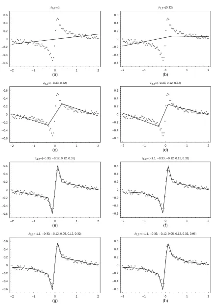
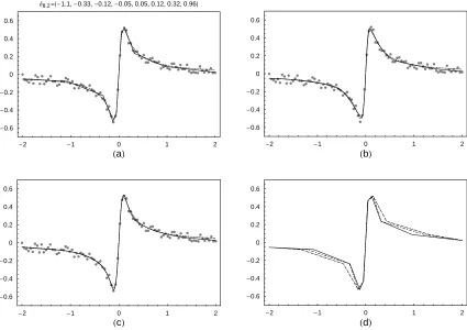
For a simulated data set, graphs of the linear spline fits, produced at each consecutive iteration in stage A of GeDS, preceding the final one, are given in Fig. 2. As can be seen, the initial straight line fit, presented in Fig. 2 (a), is sequentially improved by adding knots, one at each iteration, to reach the fit f`Hd8,2;xL, plotted in Fig. 3 (a), which
can not be further significantly improved by adding more knots. Applying the averaging knot location (8) to the knots d8,2 of the linear fit f
`
Hd8,2;xL, the set of knots t
è
8-Hn-2L,n of the quadratic, n=3, and cubic, n=4, fits, f`Hèt8-Hn-2L,n;xL, are defined. The LS spline fits
f`Itè8-Hn-2L,n,q
`
;xM, resulting from stage B of GeDS, are plotted in Fig. 3 (b) and (c) for
n=3 and n=4, respectively. The polygons CfHté
7,3,a`;xL and CfHt è
7,3,a`;xL, plotted in Fig. 3
(d), using dot-dashed and dashed lines, and obtained with ét7,3 as the solution of (7) and
with tè7,3, calculated using (8), are seen to be very close to each other and also close to
the initial control polygon f`Hd8,2,a`; xL. The final LS fits, f
`
Hét7,3;xL and f
`
Htè7,3; xL,
obtained with the optimal knots té7,3 and with the knots t
è
7,3, according to the averaging
knot location method (8), have close L2-errors, respectively 0.2798 and 0.2944, which
confirms that tè7,3 approximates very well the optimal set of knots t
é
-2 -1 0 1 2
HgL
-0.6 -0.4 -0.2 0 0.2 0.4 0.6
d6,2=81.1,-0.33,-0.12, 0.05, 0.12, 0.32<
-2 -1 0 1 2
HhL
-0.6 -0.4 -0.2 0 0.2 0.4 0.6
d7,2=8-1.1,-0.33,-0.12, 0.05, 0.12, 0.32, 0.96<
-2 -1 0 1 2
HeL
-0.6 -0.4 -0.2 0 0.2 0.4 0.6
d4,2=8-0.33,-0.12, 0.12, 0.32<
-2 -1 0 1 2
HfL
-0.6 -0.4 -0.2 0 0.2 0.4 0.6
d5,2=8-1.1,-0.33,-0.12, 0.12, 0.32<
-2 -1 0 1 2
HcL
-0.6 -0.4 -0.2 0 0.2 0.4 0.6
d2,2=8-0.33, 0.32<
-2 -1 0 1 2
HdL
-0.6 -0.4 -0.2 0 0.2 0.4 0.6
d3,2=8-0.33, 0.12, 0.32<
-2 -1 0 1 2
HaL
-0.6 -0.4 -0.2 0 0.2 0.4 0.6
d0,2=8<
-2 -1 0 1 2
HbL
-0.6 -0.4 -0.2 0 0.2 0.4 0.6
d1,2=80.32<
Fig. 2. The linear spline fits, obtained at each consecutive iteration in stage A, except the final one
[image:18.595.81.517.90.714.2]-2 -1 0 1 2
HcL
-0.6 -0.4 -0.2 0 0.2 0.4 0.6
-2 -1 0 1 2
HdL
-0.6 -0.4 -0.2 0 0.2 0.4 0.6
-2 -1 0 1 2
HaL
-0.6 -0.4 -0.2 0 0.2 0.4 0.6
d8,2=8-1.1,-0.33,-0.12,-0.05, 0.05, 0.12, 0.32, 0.96<
-2 -1 0 1 2
HbL
-0.6 -0.4 -0.2 0 0.2 0.4 0.6
Fig. 3. The final GeD spline fits: (a) linear; (b) quadratic; (c) cubic; (d) graphs of f`Hd8,2,a`;xL - the
solid line, CfIté
8-Hn-2L,n,a`;xM - the dot-dashed line and CfIt
è
8-Hn-2L,n,a`;xM - the dashed line; The dotted curve
in (a), (b), (c) is the true function.
The details of the final linear fit, and its corresponding quadratic and cubic spline fits are presented in Table 2.The computation time for the three fits is less then a second (0.89 sec. on a PC, Pentium IV, 1.4 Ghz, 512 RAM). Note that the values for the parameters
aexit and b are the default preassigned values 0.9, 0.5 (see Kaishev et al. 2006 for more
detailed comments on the effect of the choice of aexit and b). The parameter b is
defined and discussed in step 5 of Stage A (see Appendix A). As can be seen, the func-tion f is symmetric and GeDS places, symmetrically around the origin, 8, 7 and 6 knots, respectively for the linear, quadratic and cubic LS fits. As can be seen from Table 2, all the fits are of a very good quality with respect to the MSE, defined as MSE=‚
i=1
N
Hyi- f
`
HxiLL
2
ëN.
Table 2. Summary of GeD spline fits.
Fit No
Graph n k Internal knots aexit, b L2-error, MSE
1 Fig. 3,HaL 2 8 8-1.1,-0.33,-0.12,-0.05, 0.05, 0.12, 0.32, 0.96< 0.9, 0.5 0.2699, 0.000189
2 Fig. 3,HbL 3 7 8-0.69,-0.22,-0.09, 0.00, 0.09, 0.22, 0.64< 0.9, 0.5 0.2944, 0.000127
[image:19.595.85.510.94.394.2] [image:19.595.71.508.666.741.2]Based on the L2-errors for the linear, quadratic and cubic fits given in Table 2, the best
GeDS fit for this particular data set is the cubic one. We have compared it (No 3, Table 2) with the optimal cubic spline fits obtained applying the LS non-linear optimization method (NOM) and its penalized version (PNOM), due to Lindstrom (1999). The results are summarized in Table 3. As can be seen, the three fits are very close, comparing the
L2-errors, the MSE and the location of the knots. However, the GeD fit recovers best the
[image:20.595.74.413.263.339.2]original function as indicated by the corresponding MSE values. The computation time needed for GeDS is less then a second (0.89 sec.) whereas for PNOM and NOM it is respectively, 4.5 hours and 1.4 hours, using the Mathematica function NMinimize.
Table 3. The fits obtained by GeDS, PNOM and NOM.
Fit No
Method n k Internal knots L2-error, MSE
1 GeDS 4 6 8-0.51,-0.17,-0.04, 0.04, 0.16, 0.47< 0.2631, 0.000119
2 PNOM 4 6 8-0.53,-0.16,-0.06, 0.05, 0.17, 0.51< 0.2623, 0.000131
3 NOM 4 6 8-0.48,-0.15,-0.07, 0.05, 0.18, 0.40< 0.2614, 0.000154
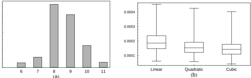
We test GeDS by fitting 1000 simulated data sets from the function f, given in Table 1. A frequency plot of the number of internal knots of the 1000 linear GeD spline fits and box plots of the MSE values of the linear, quadratic and cubic GeDS fits are presented in Fig. 4 (a) and (b).
6 7 8 9 10 11
HaL
0 50 100 150 200 250 300 350
Linear Quadratic Cubic
HbL
0.0001 0.0002 0.0003 0.0004
Fig. 4. (a): A frequency plot of the number of knots of the 1000 linear GeD spline fits; (b): Box
plots of the MSE values of the 1000 linear, quadratic and cubic GeD spline fits.
The box plots presented in Fig. 4 (b) confirm that the best GeDS fit for this particular function is the cubic one. Since the number of internal knots, k, of a quadratic (cubic) GeDS fit is always one (two) less than that of the corresponding linear fit, the frequency plot for the 1000 quadratic (cubic) GeDS fits is identical to the one in Fig. 4 (a) but over the range k =5, 6, 7, 8, 9, 10 (k =4, 5, 6, 7, 8, 9). The 1000 linear, quadratic and cubic GeD spline fits, with median number of regression functions n+k =10, have median
L2-errors 0.260, 0.267, 0.264 respectively, which are lower than 0.277, obtained by
[image:20.595.87.505.434.564.2]and Schütze (1995) is obtained starting from 15 knots and after three time-consuming knot generation, removal and relocation stages.
Constructing confidence intervals
The second part of our simulation study is devoted to the implementation of the asymp-totic results for the developed GeD spline estimator, given in Section 4. We illustrate the practical construction of finite-sample pointwise confidence intervals for the unknown function fHxL and test their performance in achieving the required nominal coverage probability levels. For this purpose, we again use the test function given in Table 1 but with normally distributed error term, ei~5H0, 0.015L, and for equally spaced design points 8xj<Nj=i1, i=1, 2, 3 with sample sizes N1=100, N2=500, N3=1000. To assess
the finite-sample performance of the constructed confidence intervals we evaluate their empirical coverage probabilities. The latter are calculated as the percentage of coverage of the true value fHxL by the 100H1- aL% confidence interval defined in (11), based on 1000 replications for each sample size, Ni. Confidence intervals are obtained using both the true s2 ("oracle" value) and its estimate, s`2, proposed by Hall et al. (1990) but only the results for the oracle values are presented. This is because our simulated results show that the estimate s`2 exhibits positive bias for small samples (see also Zhou et al., 1998) and hence, unjustifiably increases the empirical coverage probability values.
In order to compute the GeD spline estimator f`Itèl-Hn-2L,n,q
`
;xM and its variance, needed in (11), we have selected the sequence aexit1 =0.9, aexit2 =0.99, aexit3 =0.999 for the stopping rule (see step 10 of Stage A), which determines the number of knots l at exit of stage A. These values of aexit have been chosen so that the requirement of Theorems 2
and 3 with respect to the rate of growth of l with the sample size are met. Thus, the median number of knots selected by GeDS for each aexiti , i=1, 2, 3, is l1=10, l2=16,
l3=25 correspondingly.
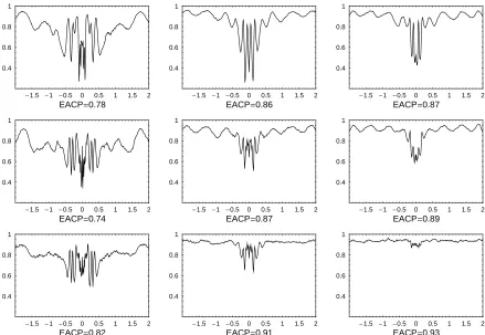
In Fig. 5 we have plotted the empirical coverage probabilities for 95% level pointwise confidence intervals as a function of x. The empirical average coverage probability (EACP) over all 8xj<Nj=i1 are also presented under each of the plots.
-1.5 -1 -0.5 0 0.5 1 1.5 2
EACP=0.82
0.4 0.6 0.8 1
-1.5 -1 -0.5 0 0.5 1 1.5 2
EACP=0.91
0.4 0.6 0.8 1
-1.5 -1 -0.5 0 0.5 1 1.5 2
EACP=0.93
0.4 0.6 0.8 1 -1.5 -1 -0.5 0 0.5 1 1.5 2
EACP=0.74
0.4 0.6 0.8 1
-1.5 -1 -0.5 0 0.5 1 1.5 2
EACP=0.87
0.4 0.6 0.8 1
-1.5 -1 -0.5 0 0.5 1 1.5 2
EACP=0.89
0.4 0.6 0.8 1 -1.5 -1 -0.5 0 0.5 1 1.5 2
EACP=0.78
0.4 0.6 0.8 1
-1.5 -1 -0.5 0 0.5 1 1.5 2
EACP=0.86
0.4 0.6 0.8 1
-1.5 -1 -0.5 0 0.5 1 1.5 2
EACP=0.87
0.4 0.6 0.8 1
Fig. 5. Empirical coverage probabilities of 95% pointwise confidence intervals, obtained by GeDS:
linear fit - first column; quadratic fit - second column; cubic fit - third column. Sample sizes:
N1=100 - first row; N2=500 - second row; N3=1000 - third row;
It is essential to mention here that, for such finite samples, it is important not only to assess the appropriate rate of growth of the number of knots but also to determine their absolute number and location. We believe that our number of knots is close to being minimal and because they are optimally located using GeDS, the 95% nominal level of the coverage probability is achieved already for sample size N =1000. Whereas, for example, if we fit a cubic spline to the data, using the same number and rate of growth of the knots but placing them uniformly, the EACP is much worse, i.e., EACP=0.20 for N =100, EACP=0.34 for N =500, EACP=0.63 for N =1000.
[image:22.595.76.515.92.395.2]-1.5 -1 -0.5 0 0.5 1 1.5 2 0.02 0.04 0.06 0.08 0.1 0.12 0.14
-1.5 -1 -0.5 0 0.5 1 1.5 2 0.02 0.04 0.06 0.08 0.1 0.12 0.14
-1.5 -1 -0.5 0 0.5 1 1.5 2 0.02 0.04 0.06 0.08 0.1 0.12 0.14 -1.5 -1 -0.5 0 0.5 1 1.5 2
-0.02 -0.01 0 0.01 0.02
-1.5 -1 -0.5 0 0.5 1 1.5 2 -0.02
-0.01 0 0.01 0.02
-1.5 -1 -0.5 0 0.5 1 1.5 2 -0.02
-0.01 0 0.01 0.02
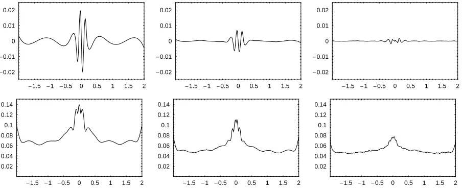
Fig. 6. Empirical bias (first row) and standard deviation (second row) of the cubic GeDS fits over
1000 replicates. Sample sizes: N1=100 - first column; N2=500 - second column; N3=1000
-third column;
In order to illustrate the local adaptability of the GeDS estimators (see stage A in Appen-dix A and Theorems 1 and 2 of Kaishev et al., 2006), in Fig. 6 we have plotted the empirical bias and standard deviation of f`Itèl-Hn-2L,n,q
`
;xM, n=4, as a function of x for
N =100, N =500, N =1000. One can see that the bias term becomes negligible com-pared to the variance term, in fact for N =1000 it is on average 300 times smaller, which corroborates the result of Theorem 2. As with the coverage probability, the bias and variance also exhibit rough behaviour around the origin which smooths out with the sample size. For brevity, we omit here the corresponding plots for the linear and qua-dratic fits.
6. Discussion.
One of the important characteristics of the GeDS estimation procedure is that it gives simultaneously linear, quadratic, cubic, etc. fits because once the LS linear spline fit in stage A is found, using the averaging knot location method (8), the knots for the higher order LS spline fits of stage B are immediately obtained. As far as we have been able to establish, no other spline fitting procedure is capable of doing this. Hence, one has the flexibility to choose the degree of the final fit providing best compromise between smoothness and accuracy.
As an alternative to the stopping rule, described in step 10 of stage A (see Appendix A), we have implemented two additional stopping criteria according to which our algorithm exits with number of knots which minimizes Stein's unbiased risk estimate (SURE) (see Stein, 1981)
(12)
RHf`L=‚
i=1
N
Iyi- f
`
Itèk,n,q
`
;xiMM
2
[image:23.595.72.524.88.273.2]or the generalized cross validation (GCV) (see e.g., Craven and Wahba, 1979)
(13) GCVHf`L=
i
k jjjjj jjj
„
i=1
N
Iyi-f
`
Itèk,n,q
`
;xiMM
2
ÅÅÅÅÅÅÅÅÅÅÅÅÅÅÅÅÅÅÅÅÅÅÅÅÅÅÅÅÅÅÅÅN ÅÅÅÅÅÅÅÅÅÅÅÅÅÅÅÅÅÅÅy
{ zzzzz
zzzìH1- ÅÅÅÅÅÅÅÅÅÅdNHkLL2
criterion. We have assumed that the minimum is attained when SURE or GCV do not decrease in two consecutive iterations in stage A. Rules (12) and (13) depend on the choice of the parameters Dand dHkL, and when D=2 and dHkL=k+1 they behave roughly as our stopping rule. The choice D=3 and dHkL=3k+1, as noted by Zhou and Shen (2001) tends to yield a smaller model, underfitting the underlying function f . For a comparative study of different model selection methods, we refer to Lee (2002). Apply-ing (12) or (13), GeDS becomes entirely automatic and can be applied if such a feature is preferred to the flexibility of controlling the output provided by our stopping rule.
We have addressed here pointwise large sample properties of this new spline estimator, such as the asymptotic behaviour of the variance and bias components of the estimation error and the construction of confidence intervals, based on the established asymptotic normality. The results of the simulation study corroborate well with the theoretical findings and support the strong practical appeal of the proposed GeD spline estimator. In conclusion, we believe that the proposed GeDS method provides a novel solution to the spline regression problem and in particular, to the problem of estimating the number and position of the knots. It is motivated by geometric arguments and can be extended to multivariate non-parametric smoothing as well as to generalized linear models. Details of how this may be done are outside the scope of this paper and are the subject of ongo-ing research.
Acknowledgements
The authors would like to acknowledge support received through a research grant from the UK Institute of Actuaries.
Appendix A
Stage A. A knot insertion scheme for variable knot, LS linear B-spline
regression.
In order to implement stage A of GeDS, an automatic knot insertion scheme is proposed to construct a variable knot, least squares, linear spline which reproduces the shape of the noise perturbed underlying function f , based on the data set 8xi, yi<iN=1. The