Abstract: The performance of a multi-layer neural network (MLP) depends how it is optimized. The optimization of MLP including its structure is tedious one as there is no explicit rules for deciding number of layers and number of neurons in each layer. Further, if the error function is multi-modal the conventional way of using gradient descent rule may give only local optimal solutions which may result in poorer performance of the network. In this paper a novel way is adopted to optimize the MLP in which a recently developed meta-heuristic optimization technique, Gray wolf optimizer (GWO) is used to optimize the weights of the MLP network. Meta-heuristic algorithms are known to be very efficient in finding globally optimal solutions of highly non-linear optimization problems. In this work the optimization of MLP is done by variation of hidden neurons layer wise and best performance is obtained using GWO algorithm. The ultimate optimal structure of MLP network so obtained is 13-6-1 where 13 is the number of neurons in the input layer, 6 is the number of neurons in the hidden layer and 1 is the number of neuron in the output layer. Single hidden layer is found to give better results as compared to more hidden layers. The performance of the optimized GWO-MLP network is investigated on three different datasets namely UCI Cleveland Benchmark Dataset, UCI Statlog Benchmark Dataset and Ruby Hall Clinic Local Dataset. On comparison the performance of the proposed approach is found to be superior to all other already reported works in terms of accuracy and MSE.
Keywords: MSE, UCI, GWO
I. INTRODUCTION
The artificial neural network (ANN) mimics the biological neural networks in its functionality and structure. The basic element in ANN is artificial neuron. It takes input, processes it using associated weights and produces output. The multiple neurons are stacked to create a layer. The first layer is called input layer and last layer is called output layer. The number of neurons in the input layer is decided by number of input parameters. The number of neurons in the output layer is decided by number of output categories. The ANN with input and output layers is called single layer ANN.
Revised Manuscript Received on December 22, 2018.
Sandeep Patil, Research Scholar, Computer Science and Engineering Department, National Institute of Technology Silchar, Cachar, Assam, India
Nidul Sinha, Professor, Electrical Engineering Department, National Institute of Technology Silchar, Cachar, Assam, India
Biswajit Purkayastha, Associate Professor, Computer Science and Engineering Department, National Institute of Technology Silchar, Cachar, Assam, India
The advantages [1] of single layer ANN include very easy to implement, fast training, direct mapping of sigmoid output function to posterior probabilities and outputs are weighted sum of the inputs.
But for the modern applications with nonlinearly separable data and complex decision boundary, the single layer ANN proved to be inefficient. So the multi-layer ANN are applied to solve them efficiently. The layer(s) between input layer and output layer is called hidden layer(s).The artificial neural network with hidden layer(s) is called multi-layer artificial neural network. There can be one or more hidden layers depending on the complexity of the problem.
The prediction accuracy of MLP network solely depends on two major parameters [1] like neural network architecture and values of the weights. The neural network architecture is mainly described by number of hidden layers and number of neurons per hidden layer. Many researchers have done significant work in this area. In 1991 Sartori et al [4] had suggested a methodology to find the number of hidden neurons after studying multiple optimization techniques. In 1993, Arai [5] had mentioned that the sufficient number of hidden neurons can be 2/3 of input neurons using two parallel hyper plane method. In 1995, Li et al. [6] have proved that second order neural network converges faster than the network with first order. In 1999, Keeni et al. [7] had discovered the number of hidden units using pruning method; but failed to improve on generalization error and could not find the optimal solution. In 2001, Onoda [8] found the optimal number of hidden units in prediction applications using statistics. Md. Islam et al [9] proved that generalization error increased when some of the may have spurious connections. In 2006, Choi et al. [10] solved local minima problem by training each hidden layer separately. In 2008, Jiang et al. [11] invented the lower bound on the number of hidden neurons. In 2009, Shibata et al [12] showed that the hidden output connection weight becomes small as number of hidden neurons becomes large. In 2010, Doukim et al. [13] proposed the combined binary search and sequential search to find the number of hidden neurons in MLP network.
Also the heart disease predication is one of the important areas of research, The creator of the Cleveland heart disease dataset, Detrano, [14] used
logistic-regression-derived discriminant function to get 77% classification accuracy.
Novel Methodology to Optimize the
Architecture of Multi-Layer Feed Forward
Neural Network Using Grey Wolf Optimizer
(GWO-MLP)
Qing Wang et al [15] have applied collection of
Randomized Bayesian Network Classifiers to predict heart disease using heart – cleveland, heart – hungarian and heart - statlog with accuracies, 83.07, 84.67 and 83.74 respectively. R. Das et al [16] created new neural network ensemble model by combining the posterior probabilities to achieve 89.01% classification accuracy with 80.95% sensitivity and 95.91 % specificity. A.V. Senthil Kumar et al [17] combined fuzzy inference system and artificial neural networks to achieve an accuracy of 91.83% for heart disease prediction. Chen et al [18] used multilayer perceptron (MLP) to predict the heart disease with 80% accuracy.
N. Cheung et al [19] combined three classifiers of Bayes namely Naive Bayes, Bayesian Network with Naïve Dependence (BNND) and Bayesian Network with Naïve Dependence and feature selection (BNNF) algorithms and C 4.5 decision tree algorithm toget classification accuracy of 81.48%, 81.11%, 80.96%, and 81.11%, respectively. Can [20] could get 88.5 % heart disease accuracy for the MCS of parallel MLP neural networks ensembles. Anna Jurek [21] provided stack of Classification by Cluster Analysis (CBCA) approach to get prediction accuracy of 84.6 %, 84.5 %, and 84.5% of heart disease on cleveland, heart, hungarian and heart-switzerland datasets respectively.
In most of the works on MLP the optimization of the network weights is done using gradient descent rule. However, this gradient based algorithm for optimization of weights works well when the error function is quadratic or non-multimodal. But if the error function is multi-modal this algorithm will give sub-optimal results and hence, the performance will be limited. In view of the above, an urge is felt to optimize the weights of MLP network using modern meta-heuristic algorithms together with the structure of the network as these algorithms are reported to be very efficient
to find better solutions if not global for highly non-linear multi-modal optimization problems.
The main objectives of this work are:
1. To find the optimum architecture of the MLP network with variation of hidden neurons layer wise and also the connecting weights of the network through evaluation using modern meta-heuristic algorithm Grey wolf optimizer (GWO) at the time of training the network for prediction of heart disease.
2. To validate the optimum MLP network obtained as above on three different data sets and compare its performance with already reported ones with conventional gradient descent based MLP networks.
The rest of the paper is organized as follows: Section 3 presents the design of maiden methodology of introducing novel methodology to optimize the architecture of Multilayer Perceptron (MLP) using Grey wolf optimizer (GWO). Section 4 presents the experimental results and analysis. Section 5 brings out the conclusion.
II. NOVEL METHODOLOGY OF OPTIMIZATION
OF ARCHITECTURE OF MLP USING GREY WOLF OPTIMIZER (GWO-MLP)
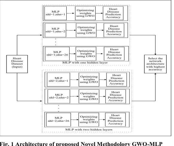
From the above literature survey the authors have decided to implement this methodology for maximum two number of hidden layers because majority of the real applications can be covered by two hidden layers. Also it is finalised that the brute force approach will be applied for hidden neurons up to double the input parameters for the exhaustive coverage. The Grey wolf optimizer is applied to every architecture to optimize the weights to find the prediction accuracy. Finally the neural network architecture with highest accuracy is selected. The taxonomy is nhl= number of hidden layer and nhn=number of hidden neurons.
MLP with one hiddeen layer
Heart Disease Dataset (Input)
Select the network architecture with highest accuracy Heart
Disease Prediction Accuracy
Heart Disease Prediction Accuracy Optimizing
weights using GWO MLP
nhl=1;nhn=1
MLP nhl=1;nhn=2
Optimizing weights using GWO
MLP nhl=1;nhn=26
Optimizing weights using GWO
Heart Disease Prediction Accuracy
Heart Disease Prediction Accuracy
Heart Disease Prediction Accuracy Optimizing
weights using GWO MLP
nhl=2;nhn=1
MLP nhl=2;nhn=2
Optimizing weights using GWO
MLP nhl=2;nhn=26
Optimizing weights using GWO
Heart Disease Prediction Accuracy
. . .
. . .
MLP with one hidden layer
[image:2.595.162.453.491.735.2]MLP with two hidden layers
Multilayer Perceptron (MLP) as Multi-layer feed forward
[image:3.595.57.282.245.387.2]Multi Layer Perceptron (MLP) is Feed-Forward Neural Network (FFNN) introduced by Rosenblatt in 1958. In MLP, the data is passed only in one direction through the network. FFNN consists of several parallel layers. The first layer is called the input layer and the last one is called output layer .The layers present between input layer and output layer are called as hidden layers. MLP consists of units called neurons connected by weighted links. Each neuron is a simple processing unit responsible for calculating its activation variable(s). Multilayer Perceptron is one of the most frequently used neural network architectures in many multi-layer artificial neural networks related applications like medical decision support systems.
Fig. 2 MLP Architecture
An activation vector is provided to the input layer which is processed by the neurons and forwarded to the hidden layer via weighted connections. Activations are calculated by hidden layer neurons and passed to the output layer. The connection weights of the network formulates the entire network function which maps input vector onto the output vector.
I) Calculation of weighted sum of inputs as mentioned in Equation (I) is,
Yj =
1
1 exp(
X
k)
1
(
. )
...(I)
mji i j
i
v z
where j=1,2,3,…..n ; m= number of input nodes ; vji=
connection weight from ith input layer node to jth hidden layer node ; zi= i
th
input ; θj=bias (threshold ) of j th
hidden node .
II) Calculation of output of hidden node as mentioned in Equation (II) is,
[image:3.595.349.483.463.607.2]yj= sigmoid(Yj)=
1
...( )
1 exp(
Y
j)
II
where j=1,2,3…n ;
III) Calculation of final output as mentioned in Equation (IV) is,
Yk=
1
(
. )
...(
)
nkj j k
j
w x
III
yk=
sigmoid(Yk)=
1
...(
)
1 exp(
Y
k)
IV
where k=1,2,3…..K ; k= number of output nodes ; wkj=
connection weight from kth hidden layer node to kth output layer node ; θk=bias (threshold ) of kth output node
Grey wolf optimizer to optimize the weights of MLP Grey wolf optimizer is a swarm based meta-heuristic proposed by Seyedali Mirjalili in 2013. This algorithm is inspired from leadership and hunting strategy followed by Grey wolves. Population of search agents is mainly divided into four groups: alpha, beta, delta ad omega.
The first three fittest wolves are defined as alpha, beta and delta respectively. Remaining wolves are omegas. Using following equations, (V) and (VI), omega wolves update their position around alpha, beta and delta wolves.
| . (t) (t) | ...(V)
( 1) (t) . | ...(VI)
p
p
D C X X
X t X A D
Where t is the current iteration,
A
2 .
a r a
1 ,C
2.
r
2,p
X
is the position of prey,X
is the position vector ofGrey wolf, a decreases linearly from 0 to 2.
r
1andr
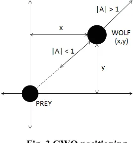
2are random vectors in [0,1]. Position updating process of Grey wolves around alpha, beta and delta is shown in figure 4 below.Fig. 3 GWO positioning
Wolf at position (X,Y) can relocate itself around the pray using equations (V) and (VI). Displacement of each wolf depends on the parameter |A|. In GWO positions of alpha, beta and delta wolves are considered as current optimum positions. Following equations, (VII), (VIII) and (IX) are used to calculate the distance of omega wolves from alpha, beta and delta.
1
| . | ...(VII)
2
|
.
| ...(VIII)
D
C X
X
3
| . | ...(IX)
D C X X
Where
X
,X
andX
are the position vectors of alpha, beta and delta respectively.X
is the current position andC
1,C
2 andC
3 are random vectors. After finding the distances, wolves need to update their positions using equations (X),(XI),(XII) and (XIII) which define the final positions of the omega wolves.1 1.( )...(X)
X X A D
2 2.( )...(XI)
X X A D
3 3.( )...(XII)
X X A D
1 2 3
(t 1) ...( ) 3
X X X
X XIII
Where, t is the current iteration number.
A
1,A
2 andA
3are random vectors. Vectors likeA
andC
are there for exploration and exploitation of search space by GWO algorithm. Exploration occurs when |A| is greater than 1 or less than -1 and when |C|>1. After each optimization iteration |A| decreases linearly and |C| is selected randomly Following steps are followed by GWO in process of optimization.1. Initialize the population randomly based on upper and lower bounds.
2. Calculate objective values (fitness) for each wolf. 3. Consider best 3 wolves as alpha, beta and delta. Based on its fitness value.
4. Using above equations, update equations of each of the omega wolf.
5. Update values of a, A and C.
6. Go to step 2 if criterion is not satisfied.
7. Return the position of alpha as the optimal solution obtained so far.
Algorithm of the proposed GWO-MLP
The algorithm of proposed GWO-MLP is as explained in figure 4.
Fig. 4 GWO MLP Algorithm
III. EXPERIMENTATION Datasets Information
This novel methodology of introducing diversity using optimization techniques to generate ensembles of base classifiers was evaluated by conducting experimentation using three different heart disease datasets. The authors have considered two UCI heart disease datasets namely Cleveland dataset and Statlog dataset and one local dataset namely Ruby hall clinic dataset. The authors also intended
to test this research work in Indian context, so they include Ruby hall clinic local dataset in this experimentation
Heart disease datasets
1. UCI Cleveland heart disease benchmark dataset [25]: For privacy purpose, the names and social security numbers of the patients are replaced. All four unprocessed files are also available in the directory, but not used in this work. The authors have
The authors have ignored those 6 records with missing values. The authors have converted this multi-class dataset into binary dataset by considering all 160 records with ‘no heart disease’ as class 0 and 137 records with any one type of heart disease among 1, 2, 3 and 4 are ‘with heart disease’ as class 1. All the 13 feature values are normalized using min max method between 0 and 1 to avoid the dominance of some of the features.
2. UCI Cleveland Statlog heart disease benchmark dataset [26]:
This heart disease dataset is in slightly different form Cleveland dataset. This dataset has no record with missing value. This dataset has 150 records with absence of heart disease as class 1 and 120 records with presence of heart disease as class 2. In this dataset also all the feature values are normalized between 0 and 1 using min max method.
3. Ruby hall clinic heart disease local dataset [27]: This heart disease dataset is collected from Ruby Hall Clinic, one of the popular heart clinics in Pune, Maharashtra, India. The main aim to include this dataset is to study this research work in Indian context. To keep compatibility with UCI Benchmark dataset, this local dataset is constructed using same 13 features. This dataset has no record with missing value. This dataset has 140 records with absence of heart disease as class 1 and 140 records with presence of heart disease as class 2. In this dataset also all the feature values are normalized between 0 and 1 using min max method.
[image:5.595.67.538.390.753.2]The summarized description of the final processed datasets is provided in table 1.
Table. 1 Heart Disease Dataset Summary Sr.
No.
Name of the dataset Number
of input features
Number of records
Number of target classes
Nature of Data
01. UCI Cleveland Benchmark Dataset 13 297 2 Normalized
02. UCI Statlog Benchmark Dataset 13 270 2 Normalized
03. Ruby Hall Clinic Local Dataset 13 280 2 Normalized
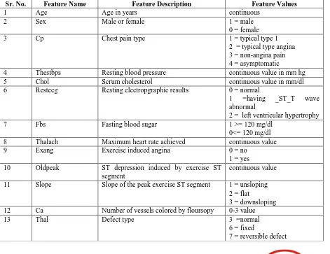
The detail description of the 13 input features is provides in Table 2 as below. Table. 2 Detail description of 13 input features
Sr. No. Feature Name Feature Description Feature Values
1 Age Age in years continuous
2 Sex Male or female 1 = male
0 = female
3 Cp Chest pain type 1 = typical type 1
2 = typical type angina 3 = non-angina pain 4 = asymptomatic
4 Thestbps Resting blood pressure continuous value in mm hg
5 Chol Scrum cholesterol continuous value in mm/dl
6 Restecg Resting electropgraphic results 0 = normal
1 =having _ST_T wave abnormal
2 = left ventricular hypertrophy
7 Fbs Fasting blood sugar 1 >= 120 mg/dl
0<= 120 mg/dl
8 Thalach Maximum heart rate achieved continuous value
9 Exang Exercise induced angina 0 = no
1 = yes 10 Oldpeak ST depression induced by exercise ST
segment
continuous value
11 Slope Slope of the peak exercise ST segment 1 = unsloping 2 = flat
3 = downsloping
12 Ca Number of vessels colored by floursopy 0-3 value
13 Thal Defect type 3 =normal
6 = fixed
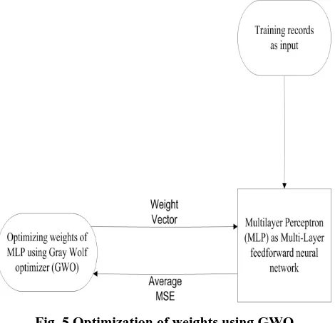
Applying Optimization Techniques to neural network Researchers have already used different optimization techniques to train the neural networks. In this experiment the concerned optimization techniquesGWO completely replace the learning algorithm of the particular neural network MLP. Important step to train a neural network with a meta-heuristic algorithm is problem representation. The MLP can be represented in a way that is suitable for optimization technique. The GWO, optimization technique is used to find the set of weights so that theMLP provides the highest approximation.
Hence, weights of MLP neural network are provided to concern optimization technique in the form of a vector. Vector can be represented by equation (XIV) as given below.
1,1 1,2 ,c
{ } {W , W , , W }...(XIV)n
V W
Where, n is the number of input nodes, Wij represents the
connection weight of ith neuron from input layer to jth neuron in competitive layer. There are total c number of neurons in competitive layer. The applied optimization technique needs an objective function which considers for optimization of values of vector V. Computing the weights to achieve the highest classification rate is the task of optimization technique. Any neural network can be evaluated based on MSE (Mean Square Error). As the all three neural networks are provided by all the training samples hence the objective will be to minimize the average MSE. Training samples are applied to the neural network and based on target values of those training samples, average MSE is calculated. Following equation (XV) is used to calculate the average MSE.
2
1
(P )
m
i i i
T MSE
m
……….(XV)Where m is the number of training samples, Pi and Ti are
[image:6.595.53.288.520.747.2]the class predicted by particular neural network and target class for ith training sample respectively.
Fig. 5 Optimization of weights using GWO Above figure 5 shows how the the weights of MLP are optimized with the help of optimization technique, GWO.
The GWO optimization technique provides weights to the MLP neural network and receives the average MSE from the particular neural network According to average MSE, optimization technique updates the position of its search agents. Ultimately it updates the vector that contains weights of the neural network. This process iterates for predefined number of iterations. Each iteration minimizes the value of MSE. This results in increase in the classification rate of neural network over the training samples.
The authors have worked with a fivefold cross-validation strategy to avoid imbalanced results. The authors have implemented this research work in the MATLAB 2013 on Windows XP operating system and run it in a Intel Core 2 CPU T5500 (1.6 GHz) PC equipped with 2048 MB of RAM .
Result Analysis
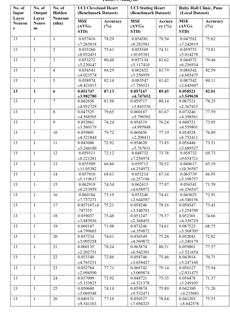
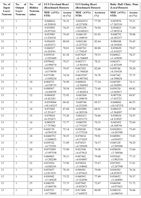
In this work the optimization of MLP is done first considering one hidden layer and number of neurons is varied from 1 to 26 (double the number of inputs) and best performance is obtained using GWO algorithm i.e. 6 neurons. Then keeping the first hidden layer with 6 neurons the number of neurons in second hidden layer is varied from 1 to 26 and performance is obtained using GWO algorithm. The ultimate optimal structure of MLP network obtained is 13-6-1 where 13 is the number of neurons in the input layer, 6 is the number of neurons in the hidden layer and 1 is the number of neuron in the output layer.
The two performance measuresused are heart disease prediction accuracy and Mean Square Error of the network. It is observed from table 3 and table 4 that the MLP architecture 13-6-1 gives highest accuracy of 89.45 % with MSE of 0.057167 for Statlog dataset. Also the same architecture is providing best results for Cleveland dataset with accuracy of 87.13 % and MSE of 0.051747 and Ruby hall clinic dataset with accuracy of 82.01 % and MSE of 0.058521. Also for majority architectures, it is observed that Statlog dataset is providing better results than other two datasets as it is processed and binary class dataset. The performance on Ruby hall clinic data set is not as good as on other two data sets because of the difference in the environment, food habits and other social factors of the people in the regions from which data are taken. First two data sets are from European region and third one is from Asian sub-continent.
Table. 3 Analysis No. of Input Layer Neuron s No. of Output Layer Neuro ns No. of Hidden Neurons (nhn)
UCI Cleveland Heart (Benchmark Dataset)
UCI Statlog Heart (Benchmark Dataset)
Ruby Hall Clinic, Pune (Local Dataset) MSE (AVG± STD) Accuracy (%) MSE (AVG± STD) Accura cy (%) MSE (AVG± STD) Accuracy (%)
13 1 1 0.057416 ±7.265018
78.29 0.054381 ±8.283581
79.54 0.047562 ±7.242019
75.62
13 1 2 0.035260 ±8.032451
75.61 0.055369 ±10.05381
74.31 0.059753 ±5.014278
73.81
13 1 3 0.053272 ±5.230147
80.48 0.057134 ±5.117410
81.62 0.044572 ±6.256934
79.44
13 1 4 0.036541 ±4.023574
84.29 0.062452 ±5.256959
83.79 0.086542 ±4.603475
82.59
13 1 5 0.058974 ±8.421013
82.14 0.083547 ±7.756521
81.42 0.087542 ±2.645607
80.11
13 1 6 0.051747 ±3.982780
87.13 0.057167 ±4.747652
89.45 0.058521 ±3.549630
82.01
13 1 7 0.042658 ±4.952729
81.98 0.059717 ±3.843536
80.14 0.087521 ±2.367415
78.25
13 1 8 0.047525 ±4.568505
79.65 0.060187 ±5.796503
81.67 0.073246 ±4.398561
77.59
13 1 9 0.052061 ±3.560179
74.24 0.054319 ±4.995848
76.24 0.048721 ±4.559801
73.05
13 1 10 0.059801 ±4.521844
79.72 0.060456 ±2.208411
77.19 0.034528 ±6.752411
76.89
13 1 11 0.043086 ±5.244180
72.92 0.054620 ±5.767631
73.85 0.056446 ±3.689327
73.51
13 1 12 0.059311 ±8.221281
72.12 0.048732 ±7.256974
73.78 0.058732 ±9.654721
69.73
13 1 13 0.055509 ±11.05382
66.86 0.059712 ±6.254972
70.52 0.048617 ±10.36587
65.19
13 1 14 0.057810 ±5.119617
68.61 0.053214 ±6.257196
67.34 0.065739 ±5.198757
66.95
13 1 15 0.062919 ±6.233959
74.54 0.062413 ±4.658972
77.97 0.036541 ±6.236547
71.59
13 1 16 0.060184 ±7.757271
73.19 0.053246 ±2.644587
74.41 0.043625 ±8.540156
72.91
13 1 17 0.057167±4 .747355
75.21 0.058246 ±3.546781
78.16 0.050347 ±3.254780
73.43
13 1 18 0.059037 ±3.885936
75.48 0.051247 ±2.368455
79.57 0.052301 ±4.358729
74.66
13 1 19 0.060187 ±4.799603
71.98 0.073246 ±4.359872
74.61 0.087525 ±3.568705
68.75
13 1 20 0.057234 ±3.995258
74.61 0.036549 ±4.569872
75.28 0.052041 ±3.240179
72.82
13 1 21 0.060135 ±2.202751
78.24 0.065874 ±6.542381
80.31 0.059801 ±3.521654
77.57
13 1 22 0.053340 ±4.765231
72.86 0.058746 ±3.658427
75.46 0.043014 ±5.247160
70.71
13 1 23 0.052784 ±2.094590
77.71 0.068742 ±3.069874
79.14 0.056127 ±2.031475
75.94
13 1 24 0.057009 ±5.153825
72.92 0.048721 ±4.521378
75.35 0.056478 ±5.249103
71.37
13 1 25 0.050660 ±5.069548
74.14 0.059874 ±9.532471
75.89 0.042380 ±4.235681
71.28
13 1 26 0.049131 ±9.541163
77.10 0.050327 ±7.694325
78.64 0.041203 ±8.642576
Table. 4 Result Set of 2 Hidden Layers
No. of Input Layer Neurons
No. of Output Layer Neurons
No. of Hidden Neurons (nhn)
UCI Cleveland Heart (Benchmark Dataset)
UCI Statlog Heart (Benchmark Dataset)
Ruby Hall Clinic, Pune (Local Dataset)
MSE (AVG± STD)
Accura cy (%)
MSE (AVG± STD)
Accuracy (%)
MSE (AVG± STD)
Accura cy (%)
13 1 1 0.048616 ±8.295018
76.32 0.0545231 ±8.237420
77.50 0.025876 ±7.242310
75.21
13 1 2 0.035893 ±8.075241
74.25 0.051258 ±10.045621
76.94 0.056823 ±5.985214
71.60
13 1 3 0.053985 ±5.236534
79.45 0.046139 ±5.108910
81.03 0.048752 ±6.202357
78.88
13 1 4 0.056439 ±4.032571
80.69 0.062140 ±5.257523
82.64 0.086548 ±4.103456
76.45
13 1 5 0.068227 ±9.254761
78.01 0.045761 ±7.750347
80.88 0.058620 ±2.610327
79.67
13 1 6 0.059510 ±3.852469
81.38 0.057629 ±4.744689
79.53 0.049621 ±3.145030
78.27
13 1 7 0.078642 ±4.998574
79.27 0.042717 ±3.841016
78.21 0.062471 ±2.452109
77.63
13 1 8 0.047651 ±4.578930
79.47 0.067203 ±5.768420
82.60 0.058746 ±4.336520
78.20
13 1 9 0.075380 ±3.058234
74.24 0.0432587 ±4.987562
76.78 0.047542 ±4.598624
75.75
13 1 10 0.068723 ±4.528753
76.98 0.068624 ±2.204562
77.24 0.045305 ±6.542091
74.11
13 1 11 0.098567 ±4.268705
70.54 0.050352 ±5.862014
71.68 0.059120 ±3.645617
69.82
13 1 12 0.068420 ±9.423281
72.92 0.043204 ±5.298674
73.19 0.087520 ±7.652721
69.87
13 1 13 0.0358964 ±10.145237
68.42 0.049746 ±6.252203
69.57 0.048602 ±10.347274
66.53
13 1 14 0.075462 ±5.351417
67.68 0.053896 ±6.205324
68.91 0.086523 ±5.564207
67.80
13 1 15 0.078624 ±6.235471
75.28 0.062413 ±4.651372
76.86 0.038624 ±4.218547
74.55
13 1 16 0.068529 ±7.757862
73.77 0.046530 ±2.753247
74.33 0.043452 ±8.548756
72.64
13 1 17 0.042170 ±4.963218
75.14 0.058246 ±3.575324
72.08 0.0542031 ±4.265380
73.69
13 1 18 0.0468752 ±3.848625
78.55 0.078634 ±4.375455
79.91 0.048901 ±4.036527
73.85
13 1 19 0.058742 ±4.753201
71.09 0.074523 ±4.745628
74.57 0.045128 ±5.569306
70.29
13 1 20 0.0572689 ±5.997558
75.88 0.023546 ±4.475621
76.28 0.058620 ±3.740546
73.04
13 1 21 0.060865 ±5.202240
78.21 0.067462 ±6.034087
79.40 0.052641 ±3.862534
77.15
13 1 22 0.053924 ±4.842101
73.96 0.078654 ±3.358602
75.67 0.057691 ±5.247590
71.81
13 1 23 0.053657 ±2.013255
78.10 0.096581 ±3.075412
79.68 0.036582 ±4.035875
76.24
13 1 24 0.056942 ±5.145628
75.22 0.040562 ±5.324596
77.80 0.054652 ±5.244983
76.37
13 1 25 0.046250 ±5.064756
73.73 0.057842 ±9.852471
72.67 0.044368 ±4.875421
71.72
13 1 26 0.047521 ±9.754803
77.97 0.017496 ±7.645872
80.09 0.048210 ±6.686516
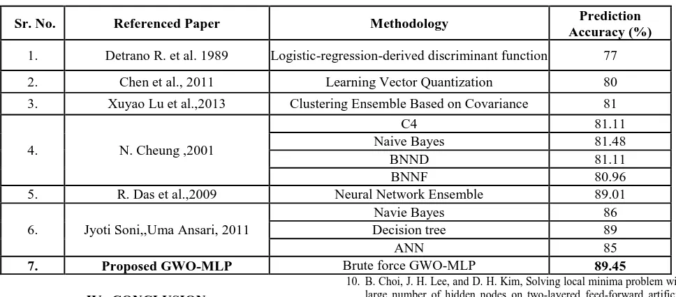
Table. 5 Comparison with existing system
Sr. No. Referenced Paper Methodology Prediction
Accuracy (%) 1. Detrano R. et al. 1989 Logistic-regression-derived discriminant function 77
2. Chen et al., 2011 Learning Vector Quantization 80
3. Xuyao Lu et al.,2013 Clustering Ensemble Based on Covariance 81
4. N. Cheung ,2001
C4 81.11
Naive Bayes 81.48
BNND 81.11
BNNF 80.96
5. R. Das et al.,2009 Neural Network Ensemble 89.01
6. Jyoti Soni,,Uma Ansari, 2011
Navie Bayes 86
Decision tree 89
ANN 85
7. Proposed GWO-MLP Brute force GWO-MLP 89.45
IV. CONCLUSION
The authors have proposed a novel optimization methodology, meta-heuristic algorithm for optimization of MLP network for accurate prediction of heart disease. The recently reported meta- heuristic algorithm GWO is used for obtaining the optimum architecture by brute force method to generate various architectures of MLP. The performance of the GWO-MLP is experimented on three heart disease data sets i.e. Cleveland, Statlog and Ruby Hall Clinic Pune dataset and compared with the already reported ones with gradient descent MLP networks for prediction of heart disease. It is observed that the performance of the proposed GWO-MLP network is superior to all the reported ones in terms of accuracy and MSE. Further, it is found that in all architectures of MLPsingle hidden layer is sufficient to approximate the search space to give optimum results with when optimized with GWO because this algorithm is having more explorative and exploitative features.
REFERENCES
1. Steve Renals, Multi-layer Neural Networks, 2011, pp. 1-29.
2. John A. Bullinaria, Introduction to Neural Networks, Bias and Variance, Under-Fitting and Over-Fitting, 2004, pp. 1-12.
3. Michał Woz´niak, Manuel Graña, Emilio Corchado, A survey of multiple classifier systems as hybrid systems, Information Fusion 16 (2014) 3–17.
4. M. A. Sartori and P. J. Antsaklis, A simple method to derive bounds on the size and to train multilayer neural networks, IEEE Transactions on Neural Networks, 2 4 (1991) 467– 471.
5. M. Arai, Bounds on the number of hidden units in binary valued three-layer neural networks, Neural Networks 6 6 (1993) 855–860.
6. J. Y. Li, T. W. S. Chow and Y. L. Yu, Estimation theory and optimization algorithm for the number of hidden units in the higher-order feedforward neural network, in: Proceedings of the IEEE International Conference on Neural Networks, 3 1995, pp. 1229-1233 7. K. Keeni, K. Nakayama and H. Shimodaira, Estimation of initial
weights and hidden units for fast learning of multi-layer neural networks for pattern classification, in: Proceedings of the International Joint Conference on Neural Networks (IJCNN ’99), 3 1999, pp. 1652– 1656
8. T. Onoda, Neural network information criterion for the optimal number of hidden units, IEEE International Conference on Neural Networks,1995, pp. 275– 280.
9. M. M. Islam and K. Murase, A new algorithm to design compact two-hidden-layer artificial neural networks, Neural Networks 14 9 (2001) 1265–1278.
10. B. Choi, J. H. Lee, and D. H. Kim, Solving local minima problem with large number of hidden nodes on two-layered feed-forward artificial neural networks, Neurocomputing 71 16-18 (2008) 3640–3643. 11. N. Jiang, Z. Zhang, X. Ma, and J. Wang, The lower bound on the
number of hidden neurons in multi-valued multi-threshold neural networks, in: Proceedings of the 2nd International Symposium on Intelligent Information Technology Application (IITA’08), 2008, pp. 103–107.
12. K. Shibata and Y. Ikeda, Effect of number of hidden neurons on learning in large-scale layered neural networks, in: Proceedings of the ICROS-SICE International Joint Conference 2009 (ICCASSICE ’09), 2009, pp. 5008–5013.
13. C. A. Doukim, J. A. Dargham, and A. Chekima, Finding the number of hidden neurons for an MLP neural network using coarse to fine search technique, in : Proceedings of the 10th International conference on Information Sciences, Signal Processing and Their Applications (ISSPA ’10), 2010, pp. 606–609.
14. Newman D.J., Hettich S., Blake C.L., Merz C.J., UCI repository of machine learning databases, Department of Information and Computer Science, University California Irvine, 1998.
15. Qing Wang, Ping Li, Randomized Bayesian Network Classifiers, in MCS 2013: Proceedings of the Eleventh International Workshop on Multiple Classifier Systems, Nanjing, China, Springer-Verlag , 2013, pp. 319-330.
16. R. Das, I. Trukoglu and A. Sengur, Effective diagnosis of heart disease through neural networks ensembles, Expert Systems with Applications 36 (2009) 7675-7680.
17. A.V. Senthil Kumar, Diagnosis of Heart Disease using Fuzzy Resolution Mechanism, Journal of Artificial Intelligence (2012) 47-55 18. A.H. Chen, S.Y. Huang, P.S. Hong, C.H. Cheng and E.J. Lin, HDPS:
Heart Disease Prediction System, in: proceeding of International Conference Computing in Cardiology, 2011, pp. 557-560.
19. N. Cheung, Machine learning techniques for medical analysis, in : Thesis of School of Information Technology , University of Queenland, 2001, pp. 58-61
20. Mehmet Can, Committee Machine Networks to Diagnose Cardiovascular Diseases, Southeast Europe Journal of Soft Computing (2013) 76-83.
21. Anna Jurek, Yaxin Bi, Shengli Wu and Chris Nugent, Classification by Cluster analysis: A New Meta-Learning Based Approach, in MCS 2011: proceedings of the tenth International Workshop on Multiple Classifier Systems, Naples, Italy Springer-Verlag, 2011, pp. 259-268. 22. Xuyao Lu, Yan Yang, Hongjun Wang, Selective Clustering Ensemble