This is a repository copy of
Probabilistic partial least squares model: Identifiability,
estimation and application
.
White Rose Research Online URL for this paper:
http://eprints.whiterose.ac.uk/131974/
Version: Accepted Version
Article:
El Bouhaddani, S, Uh, H-W, Hayward, C et al. (2 more authors) (2018) Probabilistic partial
least squares model: Identifiability, estimation and application. Journal of Multivariate
Analysis, 167. pp. 331-346. ISSN 0047-259X
https://doi.org/10.1016/j.jmva.2018.05.009
© 2018 Elsevier Inc. All rights reserved. This manuscript version is made available under
the CC-BY-NC-ND 4.0 license http://creativecommons.org/licenses/by-nc-nd/4.0/
[email protected] https://eprints.whiterose.ac.uk/ Reuse
This article is distributed under the terms of the Creative Commons Attribution-NonCommercial-NoDerivs (CC BY-NC-ND) licence. This licence only allows you to download this work and share it with others as long as you credit the authors, but you can’t change the article in any way or use it commercially. More
information and the full terms of the licence here: https://creativecommons.org/licenses/
Takedown
If you consider content in White Rose Research Online to be in breach of UK law, please notify us by
Probabilistic partial least squares model:
Identifiability, estimation and application
Said el Bouhaddania,∗, Hae-Won Uhb,a, Caroline Haywarde, Geurt Jongbloedc, Jeanine Houwing-Duistermaatd,a
aDepartment of Medical statistics and bioinformatics, Leiden University Medical Center, The Netherlands
bDepartment of Biostatistics and Research Support UMC Utrecht, div. Julius Centrum, University Medical Center Utrecht, The Netherlands cDepartment of Applied Mathematics, Delft University of Technology, The Netherlands
dDepartment of Statistics, University of Leeds, United Kingdom
eMRC Human Genetics Unit, Institute of Genetics and Molecular Medicine, University of Edinburgh, Scotland
Abstract
With a rapid increase in volume and complexity of data sets, there is a need for methods that can extract useful information, for example the relationship between two data sets measured for the same persons. The Partial Least Squares (PLS) method can be used for this dimension reduction task. Within life sciences, results across studies are compared and combined. Therefore, parameters need to be identifiable, which is not the case for PLS. In addition, PLS is an algorithm, while epidemiological study designs are often outcome-dependent and methods to analyze such data require a probabilistic formulation. Moreover, a probabilistic model provides a statistical framework for inference. To address these issues, we develop Probabilistic PLS (PPLS). We derive maximum likelihood estimators that satisfy the identifiability conditions by using an EM algorithm with a constrained optimization in the M step. We show that the PPLS parameters are identifiable up to sign. A simulation study is conducted to study the performance of PPLS compared to existing methods. The PPLS estimates performed well in various scenarios, even in high dimensions. Most notably, the estimates seem to be robust against departures from normality. To illustrate our method, we applied it to IgG glycan data from two cohorts. Our PPLS model provided insight as well as interpretable results across the two cohorts.
Keywords: Dimension reduction, EM algorithm, Identifiability, Inference, Probabilistic partial least squares
1. Introduction
With the exponentially growing volume of data sets, multivariate methods for reducing dimensionality are an important research area in statistics. For combining two data sets, Partial Least Squares (PLS) regression [28] is a popular dimension reduction method [1]. PLS decomposes variation in each data set in a joint part and a residual part. The joint part is a linear projection of one data set on the other that best explains the covariance between the two data sets. These projections are obtained by iterative algorithms, such as NIPALS [28]. Partial Least Squares is popular in chemometrics [3]. In this field, the focus is on development of algorithms with good prediction performance, while the underlying model is less important. For applications in life sciences, interpretation of parameter estimates is necessary to gain understanding of the underlying molecular mechanisms.
For interpretation, a model needs to be identifiable. A model is said to be unidentifiable if the model corresponds to more than one set of parameter values. For PLS, rotation of the parameters does not change the model [26]. Hence, PLS does not provide an identifiable model. By constraining the parameter space, identifiability can be obtained. This involves solving a challenging optimization problem, since PLS requires estimating a structured covariance matrix [19].
For many problems in life sciences the study design needs to be accounted for, and algorithmic approaches such as PLS cannot be applied. Hence, a probabilistic formulation is necessary. Since likelihood method provides asymptotic standard errors of parameter estimates, computer-intensive resampling procedures can be avoided.
∗Corresponding author
Also for other dimension reduction techniques, probabilistic methods have been developed. In 1999, Tipping and Bishop [23] developed the Probabilistic Principal Component Analysis (PPCA), in order to deal with missing data and dependent samples. In 2005, Bach and Jordan [2] developed Probabilistic Canonical correlation analysis (PCCA). However, for both PPCA and PCCA the model parameters are not identifiable, since rotation of the parameters does not change the model [2, 23]. In addition, in 2015, simultaneous envelopes models have been developed [4] for ‘low-dimensional’ settings. Further, Probabilistic PLS Regression and Probabilistic PLS have been proposed [14, 30]. For all these approaches, the model parameters are not identifiable.
In this paper we propose the Probabilistic Partial Least Squares (PPLS) model and show that the model pa-rameters are identifiable up to a sign. We propose to maximize the PPLS likelihood with an EM algorithm that decouples the likelihood into several factors involving distinct sets of parameters. In the M step, a constrained optimization problem is solved by using a matrix of Lagrange multipliers.
The rest of the paper is organized as follows: In Section 2 we develop the PPLS model and establish identifiabil-ity of the model parameters. We develop an efficient algorithm for estimating the PPLS parameters. In Section 3 we study the performance of the PPLS estimators via simulations. In Section 4 we illustrate the PPLS model with two data matrices from two cohorts. We finish with a discussion.
2. Model and estimation
2.1. The PPLS model
Let xandybe two random row-vectors of dimension p andq, respectively. The Probabilistic Partial Least
Squares (PPLS) model describes the two random vectors in terms of a joint part and a noise part. The joint part consists of correlated latent vectors, denoted bytandu, while the noise part consists of isotropic normal random vectors referred to ase, f andh. The dimension oft andu is denoted byr. The PPLS model describing the relationship betweenx,yand the joint and noise parts is
x=tW⊤+e, y=uC⊤+f, u=tB+h. (1)
Specifically,e=(e1, . . . ,ep), f =(f1, . . . ,fq) andh=(h1, . . . ,hr) are independent with zero mean and referred
to as noise variables. The distributions ofe, f andh are multivariate normal with positive definite covariance matrix proportional to the identity matrix,
e∼ N(0, σ2eIp), f ∼ N(0, σ2fIq), h∼ N(0, σ2hIr).
The latent vectort=(t1, . . . ,tr) is anr-dimensional multivariate normal vector with with zero mean and diagonal
positive definite covariance matrixΣt=diag(σ2t1, . . . , σ
2
tr), so
t∼ N(0,Σt). (2)
The matrixB=diag (b1, . . . ,br) is a diagonal matrix of sizer, containing regression coefficients ofuont. Finally W (p×r) andC (q×r) are parameter matrices, referred to as loadings. The PPLS model for the random p -dimensional row-vectorxand randomq-dimensional row-vectoryis given in Eq. (1). Letθbe the parameters of the PPLS model, i.e.,
θ=(W,C,B,Σt, σe, σf, σh). (3)
The PPLS model and its parameters are formulated conditional on the value of the dimension of the latent spacer. The PPLS model (1) assumes a multivariate normal distribution for the observable random vectorsxandy. The covariance betweenxandyis modeled by the regression of the latent vectoruont. The distribution of (x,y) is
N(0,Σ) with density given, forx∈Rpandy∈Rq, by
f(x,y)=(2π)−(p+q)/2|Σ|−12e(x,y)Σ
−1(x,y)⊤
,
and covariance matrix
Σ = Σx Σx,y Σy,x Σy
!
= WΣtW ⊤+σ2
eIp WΣtBC⊤
CBΣtW⊤ C(B2Σt+σ2hIr)C⊤+σ2fIq
!
. (4)
2.2. Identifiability of probabilistic PLS
To establish identifiability of the PPLS model, some assumptions about its parameters have to be made. First, we assume that 0 <r <min(p,q). Second, we assume that the diagonal elements ofBare positive,bk >0 for k∈ {1, . . . ,r}. This will not restrict the model, sincetkbkis equal to−tkbkin distribution. To identify the order
of the loading vectors, the elements of (σ2
tkbk) r
k=1are assumed to be strictly decreasing withk. Finally, we assume that the loading matricesW andCare orthogonal, i.e.,W⊤W =C⊤C=I
r. Together with the diagonality ofΣtin
(2), it implies identifiability of all parameters up to sign. This is shown in the following theorem.
Theorem 1. Let r be fixed such that0 <r <min(p,q). Let(x,y)1 and(x,y)2 be generated by the PPLS model
(1)having covariance matrixΣ1andΣ2with underlying parametersθ1andθ2as defined in(3), respectively. Then
Σ1= Σ2implies that W1 =W2∆, C1=C2∆for some diagonal matrix∆with on the diagonal elementsδi∈ {−1,1},
for i∈ {1, . . . ,r}, and all other parameters inθ1andθ2are equal.
The formal proof is given in Appendix B. Identifiability up to sign can be represented by a diagonal orthogonal matrix, namely a diagonal matrix with diagonal elements in{−1,1}. For example, taking the model forxin (1), we may substituteWbyWRS andtbytRS, whereRS is a diagonal orthogonal matrix, and get
x=tRSR⊤SW
⊤ +e=
r X
j=1
tj(RS)2j jw
⊤
j +e.
Since (RS)2j j =1 and the distribution oftjand−tjis the same, the right-hand side reduces to the original model for xin (1). Note that the PPLS model is not invariant under general rotation matrices. Take a general rotation matrix
R, then we still get
x=tW⊤+e=tRR⊤W⊤+e,
sinceRR⊤ =Ir. Inspecting the covariance ofT Rwe see that cov(T R)=R⊤ΣtR, which is not diagonal ifRis not
diagonal, and violates the PPLS model assumption onΣtin Eq. (2).
2.3. Estimating the parameters
Unlike the iterative PLS methods, we propose a simultaneous approach for estimating the parameters, while taking the constraints in the PPLS model into account. Given the number of PPLS components,r, the log likelihood of an independent and identically distributed (iid) sample (X,Y)={(X1,Y1)⊤, . . . ,(XN,YN)⊤}⊤of sizeNfrom (x,y)
is
L(θ)=−N(p+q)
2 −
N
2 ln|Σ| −
N
2tr(SΣ
−1
) (5)
withS =N−1PN
i=1(Xi,Yi)⊤(Xi,Yi) andΣas in Eq. (4). To ensure empirical identifiability, we assume thatr<N.
Note that the data dimensionalitypandqmay be larger thanN. For estimation ofθ, maximum likelihood is used. The log likelihood (5) depends in a non-linear way on the theoretical covariance matrixΣ, which contains the loadings and variances. Optimizing this function directly is a non-trivial task, especially in high dimensions (i.e. whenpandqare large). However, the PPLS model allows for a more simple (but iterative) optimization approach. Indeed, the maximum likelihood estimates forθare a least squares type solution if the latent variablestanduare observed, as the model forxandyin (1) involves knowntandu. In contrast, knowingθallows for reconstruction oft anduby computing their conditional means given xandy. Alternating these two scenarios is actually an Expectation-Maximization (EM) [5] algorithm, with observed data (x,y) and missing data (t,u).
The EM algorithm. The joint distribution of the complete data (x,y,t,u) can (with abuse of notation) be
decom-posed as
f(x,y,t,u)= f(x|t)f(y|u)f(u|t)f(t). (6)
This follows from
f(x,y,t,u)= f(x,y|t,u)f(t,u)= f(x|t,u)f(y|t,u)f(t,u).
andyandtare independent givenu. The last factor can be rewritten as f(u|t)f(t), yielding Eq. (6). The logarithm of the first three factors in the product in (6) can be written as
lnf(X|T)=− N p
2πσ2
e
− 1
2σ2
e N X
i=1
||Xi−TiW⊤||2,
lnf(Y|U)=− Nq
2πσ2
f
− 1
2σ2
f N X
i=1
||Yi−UiC⊤||2,
lnf(U|T)=− Nr
2πσ2
h
− 1
2σ2
h N X
i=1
||Ui−TiB||2.
Denote byLComp=lnf(X,Y,T,U) the complete data log-likelihood, and define
Q(θ)=E{LComp(θ)|X,Y, θ′},
where the expectation is taken conditional on the observed X andY, and θ′ is a fixed current estimate of the parameters. By optimizingQover all allowedθ, we get a non-negative increase in theobservedlog-likelihood
L. Moreover, by iterating this process of taking the expectation and maximizing overθ, the estimates in general converge to a stationary point or, in particular, a (possibly local) maximum ofL[5, 29]. The expectation step calculates the conditional expectation of the missing data given the observed data given byQ(θ), which may in general involve intractable integration. However, for the exponential family, in particular the multivariate nor-mal family, the complete likelihood depends on the complete data only via the sufficient statistics (calledt(x) in [5]), which are given in terms of the first and second moments of the complete data for the multivariate normal distribution. ComputingQ(θ) implies computing the expected first and second moment of the latent variables: E (T|X,Y, θ), E T⊤T|X,Y, θ
, E (U|X,Y, θ), E U⊤U|X,X, θ
and E U⊤T|X,Y, θ
; see Appendix C for details. More-over, the decomposition in (6) allows for optimization of E{lnf(X|T)}, E{lnf(Y|U)}and E{lnf(U|T)}separately, while only considering parameters involved in each factor. MaximizingQoverθyields parameter estimates for the next iteration in the EM algorithm. This leads us to the following theorem.
Theorem 2. Let X and Y be an observed data sample of size N, generated according to the PPLS model(1). Let r
be fixed such that0<r<min(N,p,q). The parameters inθcan be estimated with an EM algorithm, yielding the
following iterative scheme in k with given starting values for k=0:
Wk+1=X⊤E(T|X,Y, θk)(L⊤W)−1; Ck+1=Y⊤E(U|X,Y, θk)(L⊤C)−1;
Bk+1=E(U⊤T|X,Y, θk){E(T⊤T|X,Y, θk)}−1◦Ir; Σkt+1=
1
NE(T
⊤T|X,Y, θk
)◦Ir; (σ2h)
k+1= 1
NrtrE(H
⊤H|X,Y, θk
);
(σ2e) k+1
= 1
N ptrE(E
⊤
E|X,Y, θk); (σ2f)k+1= 1
NqtrE(F
⊤
F|X,Y, θk);
where LWand LCare such that
LWL⊤W=E(T
⊤|X,Y, θk
)X X⊤E(T|X,Y, θk), LCL⊤C=E(U
⊤|X,Y, θk
)Y Y⊤E(U|X,Y, θk).
The proof for Theorem 2 and the expressions for the conditional expectations are given in Appendix C. Note the dependency ofWk+1andCk+1on the matricesL
WandLC. These matrices ensure orthogonality ofWk+1andCk+1
in each iteration:
(Wk+1)⊤Wk+1=L−W1T˜⊤X X⊤T˜(L⊤W)−1=LW−1LWL⊤W(L
⊤
W)
−1=I
r,
where ˜T = E(T|X,Y, θk). The exact forms of L
W and LC are not unique. Two choices are the eigenvectors of
E(T⊤|X,Y, θk)X X⊤E(T|X,Y, θk) and the lower triangular matrix ofX⊤E(T|X,Y, θk) in the Cholesky decomposition. Note that these two orthogonalization matrices are straightforward to calculate with standard linear algebra tools. Since the PPLS model is identifiable, all choices forLW andLC will lead to the same optimum as the iteration
Standard errors for PPLS. Asymptotic standard errors for maximum likelihood estimators are found by inverting the observed Fisher information matrix. Following the reasoning of [16], the observed information may be given by
E{B(ˆθ)|X,Y} −E{S(ˆθ)S(ˆθ)⊤|X,Y}.
HereS(ˆθ)=∇λ(ˆθ) andB(θ)=−∇2
λ(ˆθ) are the gradient and negative of the second derivative of the log likelihood λ(θ) respectively evaluated in the MLE ˆθ. The explicit form of the asymptotic covariance matrix ofwkis given in
Appendix D. The square root of the diagonal elements are the asymptotic standard errors for the corresponding loading estimates.
Finding the number of components r. Available approaches to determine the number of PPLS componentsrare
minimizing a cross-validated loss function [9], visually inspecting eigenvalues of a covariance matrix [17], and se-lecting the number of components needed to achieve a certain proportion of variance explained by the components. In this paper we apply the last approach.
The PLS and PPLS algorithms are available asRpackages atgithub.com/selbouhaddaniunder repository
OmicsPLS and PPLS, respectively.
3. Simulation study
To evaluate the performance of the PPLS estimates, a simulation study was conducted. The aim was (1) to investigate the performance of PPLS for various scenarios, (2) to evaluate robustness of the PPLS estimates against departures from the normality assumption, (3) to compare the performance of the loading estimates with other probabilistic approaches, and (4) to compare the asymptotic PPLS standard errors with the bootstrap standard errors.
The simulated data were generated according to the PPLS model (1). The number of components was chosen to be 3, both in the data generation and in the estimation. We considered combinations of small and large sample size (N ∈ {50,500}), low and high dimensionality (p ∈ {20,1000}), and small and large proportion of noise (denoted byαn ∈ {0.1,0.5}). The robustness of PPLS was evaluated by considering four different continuous and discrete
distributions for the latent variablest,u,e, f andh; we chose the normal distribution, thetdistribution with two degrees of freedom, the Poisson distribution with rate 1, and the Binomial distribution with two trials and success probability 0.25. These distributions cover a wide range of characteristics typically observed in omics data: heavy tailed, skewed and/or discrete. The latent variables were scaled to have mean zero and variances as specified below. All scenarios are summarized in Table 1.
The true loading values per component were generated from the normal density function with parametersµand σ, denoted byN(x;µ, σ2), as follows
wj,k=N{j; (1/2+1/10j)p,1/10p}, cj,k=N{j; (3/5+1/10j)q,1/10q}.
The second columns inWandCwere orthonormalized with respect to the first columns, and the third columns were orthonormalized with respect to the first two columns; we used a Gram–Schmidt procedure for both operations. The elements of the diagonal matrixBwere set tobk =eln(1.5)−3(k−1)/10 =(1.5,1.11,0.82), forΣtwe choseσtk = e−(k−1)/10=(1,0.90,0.82).
For comparing the parameter estimates with the true values θ, we computed the bias and the variance of the
estimates. To deal with the identifiability up to sign, we multiplied each estimated loading vector by−1 if the inner product of the estimated loading vector and the true loading vector was negative. Moreover, we swapped columns inWandCto maintain the same ordering as the ordering in the true loadings. This was done to avoid inflation of the bias or variance due to a wrong sign or ordering of the individual components.
PPLS estimates were compared to PLS estimates (with orthogonal loadings, see [20] for an overview) for all
scenarios above. For comparing PPLS with PPCA and PCCA, we constructed a ‘null model’, i.e.,B=0, as well
asB,0. We used the same scenarios as above, but we only considered the normal distribution.
Regarding standard errors for PPLS loadings, we compared asymptotic standard errors (as in Section 2) and
bootstrap standard errors [27]. One set of two data matricesX andY was simulated from a PPLS model with
Table 1: Overview of the simulation scenarios. The noise level is defined as the proportion of variation in the noise matricesE,FandHrelative to the total variation inX,YandUrespectively.
Sample size N=(50, 500)
Dimensionality p=q=(20, 1000)
Noise level αn =(0.1, 0.5)
Distribution oft,u,e, f andh {N(0,1), t2, P(1), BIN(2,0.3)}
original data) were included as reference. Low and high noise levels (αn =0.1 resp. αn =0.5), and small, large
and ‘extra large’ sample sizes (N = 50, N = 500 and N = 5000, respectively) were considered. In the ‘extra
large’ sample size scenario, no simulation-based reference was calculated. The PPLS estimation algorithm was considered to be converged when either the log-likelihood increment was below 10−6, or 104EM steps were made. For each scenario, 1000 replicates are used.
3.1. Results
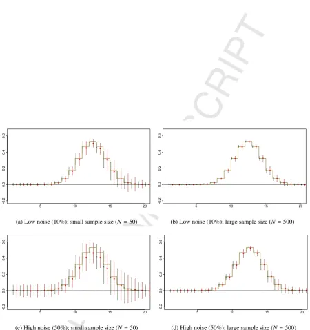
Results for the loadings. The biases and variances of the estimated first componentW1for the low dimensional
case for normally distributed latent variables are graphically depicted in Figure 1. A black dot represents the average estimated PPLS loading value across 1000 simulations, whereas the width of the black dashed vertical line equals two times the standard deviation across 1000 simulations. The red star and red dashed vertical line represent the average loading value and twice the standard deviation for the PLS estimates. The true loading values are represented by a step function with steps at each indexj∈ {1, . . . ,p}. Results for other components and scenarios are included in the Online Supplement.
Comparing the estimates for thefirstloading componentW1, a better performance of PPLS compared to PLS
was observed in terms of bias. In all scenarios the bias of the PPLS estimators were about the same as or less than the bias of the PLS estimators. Both estimators showed larger bias towards zero for higher absolute loading values. The biases decreased with a larger sample size and lower noise level. The biases of both estimators were very similar across different distributions. In the scenario where there is 50% noise and few (50) samples the variance of the PPLS estimators tended to be slightly larger than the variances of the PLS estimators when the true loading values were larger. This was observed across all distributions. The variances of the PPLS estimates were about the same or lower than the PPLS estimates in all other scenarios, where either the noise level was less or more samples were available. For both PPLS and PLS estimators the variances tended to increase with higher loading values. The variances decreased with larger sample size and lower noise level. The variances of bots estimators were very similar across different distributions. For the loading componentC1and their PLS and PPLS estimators the same conclusions were obtained.
For the second loading component W2 (shown in the Online Supplement), the biases of the PPLS loading
estimates were as good as, and often better than the PLS loading estimates, especially at lower values. In the scenarios of 50% noise and a small sample size (N=50) the bias was slightly larger for PPLS estimators compared to PLS estimates when the loading values were larger. Both estimators showed larger bias towards zero for higher loading values. The biases decreased with a larger sample size and lower noise level. For all distributions, the biases of both estimators were very similar. The variances of the PPLS estimators were as good as or lower than the PLS estimators, except in the scenario in which both the noise level was high (50%) and the sample size was small (50). In this scenario the variances of the PPLS estimators were still lower if the true loading values were close to zero, but higher for higher loading values. For both PPLS and PLS estimators the variances tended to increase with higher loading values. The variances decreased with larger sample size and lower noise level. The variances of both estimators were very similar across different distributions. For the loading componentC2and their PLS and PPLS estimators the same conclusions were obtained.
For thethirdloading componentsW3andC3 (shown in the Online Supplement), the same observations were
made as for the first loading componentsW1andC1, both for the biases as for the variances.
For the high and extra high-dimensional case, the same results were obtained for the loadingsWandC. See the Online Supplement for more details.
Table 2: Proportion of correct order of loadingsWandCacross 1000 simulation replicates. These were obtained for different values of the dimensionality (high=1000 variables, low=20 variables), sample size (large=500 subjects, small=50 subjects) and noise level (high=
50% noise, low=10% noise).
Dimensionality Sample Size Noise Level Correct Ordering Proportion
low
large low 1.000
high 0.989
small low 0.932
high 0.435
high
large low 0.990
high 0.985
small low 0.940
high 0.665
Results for the variance parameters. The performance of the estimators of the variance parametersB,σt,σe,σf
andσh were also evaluated, the results are shown in Figure 2. We did not compare with PLS as these model
parameters are not present in the PLS framework. For sake of comparison, we calculated the relative biases and variances of the estimates with respect to the true corresponding parameter value. The biases of the PPLS estimators for all variance parameters were very small for large sample size (N =500), regardless of the noise. For small sample size (N =50), the first two diagonal elements ofBandΣt were overestimated, while the last
component was underestimated. The noise parametersσeandσf were underestimated in these scenarios, while the
estimator forσhwas unbiased, except in combination with a low noise level (10%). The relative biases decreased
slightly with lower noise level, except for the earlier mentionedσh, and decreased more with larger sample size.
The relative variances of the estimators of B,Σt andσh were larger than the variances of the estimators ofσe
andσf. For B, there was a slight increase in variance across the three components. The variances decreased
slightly with lower noise and more with larger sample size. The variances slightly decreased in the scenario of high dimensionality and high noise level. The same observations were made across the different distributions.
Ordering of the loadings. We compared the ordering of the true loadingsW andCwith the ordering of the
esti-mated loadings. This provides a proportion across the 1000 simulation replicates in which the ordering matched. In Table 2, the proportion of correct orderings ofW for the scenario with normally distributed latent variables is shown for different scenarios. It can be seen that the proportion of correct orderings tends to be lower with smaller sample size and with higher noise level. Moreover, if the sample size is small, the proportion of correct orderings is much lower with higher noise. A higher dimensionality has a slightly negative impact on the correct ordering proportion when the sample size is larger, but a positive impact in the small sample size scenario. Especially, when also the noise level is high, this can be considerable. The same observations were made for the other distributions. Exactly the same proportions were observed for the loadingsC.
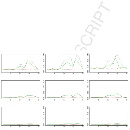
Comparison of PPLS standard errors. The results for low noise level are shown in Figure 3. In all scenarios,
the asymptotic standard errors were smaller than the bootstrap standard errors for nearly all loading elements. In particular, for high loading values the difference between asymptotic and bootstrap standard errors tended to be large. This difference decreased with larger sample size: In the ‘extra large’ sample size, the bootstrap and asymptotic standard errors had similar magnitude. Similar observations were made for other distributions. For details, see the Online Supplement.
4. Data analysis
To illustrate the Probabilistic Partial Least Squares model, we apply it to IgG glycan datasets. Glycans, in particular IgG glycans, play an important role in the innate immune system, as well as in cell signaling. IgG2 glycans are less abundant than IgG1 glycans and more difficult to measure. Therefore, by using the relationships between IgG1 and IgG2 glycans, the characteristics of IgG2 can be better estimated. Hence, we will use IgG1 as
Xmatrix, and IgG2 asYmatrix.
participants) [12]. The data matrices containing IgG1 and IgG2 glycan variables are denoted byXmandYm, with
m∈ {1,2}, wherem=1 corresponds to CROATIA Korcula andm=2 corresponds to CROATIA Vis. We apply
PPLS to IgG1 and IgG2 glycans in each cohortseparatelyand compare results.
In Figure 4, heatmaps of the correlations within and between the IgG1 and IgG2 glycans are shown, from which it is clear that there are many highly positive correlations between and within IgG1 and IgG2 in each data set. The RV coefficient [18], which generalizes thesquaredPearson correlation coefficient to two matrices, was about 0.60 and 0.45 for CROATIA Korcula and CROATIA Vis cohorts respectively.
To determine the number of latent variables to use, we considered the total amount of variance explained by the latent space relative to the total amount of variation in the data:||Tm||/||Xm||and||Um||/||Ym||form∈ {1,2}. By using
four components, at least 89% of the total variation in each of the matricesX1,X2,Y1andY2was accounted for.
For both cohorts, we fitted the PPLS models usingr =4 latent components. The amount of overlap in each
cohort, estimated by tr ˆΣx,y/tr ˆΣygiven in (4), was 58% and 46% for CROATIA Korcula and CROATIA Vis cohorts,
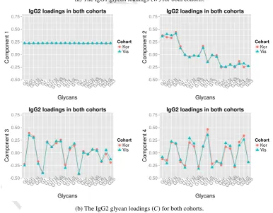
respectively. The PPLS loadings are inspected to identify which IgG glycans contribute most to this overlap. The estimated IgG1 loadings wj,k, j ∈ {1, . . . ,p}andk ∈ {1, . . . ,4}, for both cohorts and both subclasses are
depicted in Figure 5. The first joint component is proportional to the average glycan, as all glycans get about the same loading value. The second joint component involves especially G0 and G2 glycan subtypes, in which they are negatively correlated. Inspection of the loading values for the third component shows contibutions of fucosylated and non-fucosylated glycan subtypes. In the fourth component a pattern of positive and negative loading values is visible regarding the presence and absence of bisecting GlcNAc, respectively. The large loading value for G1NS is remarkable. The same conclusions hold for IgG2, as the estimated loading values were very similar. It is interesting to note that the observed patterns within components potentially reflect enzymatic synthesis where monosaccharides are added to glycan substrates [22]. Additionally, similar patterns are seen reflecting the inflammatory characteristics of glycans in aging and several different diseases [13]. Finally, the observed loading patterns were strikingly similar for both cohorts.
5. Discussion
We proposed PPLS to model the covariance matrix of two data sets. Maximum likelihood estimators for the model parameters were derived by solving a constrained optimization problem, and the parameter loadings were shown to be identifiable up to sign. This property ensures that PPLS estimates are comparable across several studies.
Our simulation study showed that the PPLS estimators had good performance and lower bias compared to PLS. Most notably, the performance of PPLS was robust to misspecification of the distribution of the variables. A smaller sample size and high noise level had a negative effect on the accuracy of the estimates, but large loading values were still non-zero. Also, compared to Probabilistic CCA estimates, the PPLS estimates were less biased and more efficient. For high-dimensional data, PCCA estimates have larger bias and higher variance. This is likely to be caused by the unstable inverse sample covariance matrix calculated when using PCCA. Moreover, if the number of variables is larger than the sample size, PCCA estimates cannot be obtained. Therefore, especially in omics data analysis, PPLS provides more robust findings.
As an illustration of the PPLS model, we analyzed IgG glycomics data from two cohorts. The high correlations in the data (Figure 4) and the use of multiple cohorts illustrate the applicability of PPLS to facilitate combination of results derived from different experimental settings. We found that the estimated loading values were almost identical across the two cohorts (Figure 5).
studies. For example, in [25], a non-probabilistic approach is pursued in a least squares estimation method using PCA. Performing data integration across studies, while taking into account uncertainties within each study, is one of our topics for future research, and will lead to more powerful analysis of the IgG glycans across cohorts.
To assess the statistical significance of loadings, the probabilistic framework provides alternative approaches to jackknifing and bootstrapping [27]. The observed Fisher information matrix can be used to estimate standard errors for individual loading parameters. For small sample sizes, bootstrap approaches appears to better reflect the uncertainty of the parameters. For large enough sample sizes, the asymptotic standard errors are close to the simulation-based standard errors. Typically, in epidemiological studies, the sample size is large enough to use asymptotic standard errors.
In this paper we ignored the fact that different biological ‘omics’ measurements have different error structures. An extension of Partial Least Squares was proposed to correct for systematic variation (variation induced by latent variables uncorrelated to the other data set) in the data sets, named Two-Way Orthogonal PLS (O2PLS) [8, 24]. Such an extension can be pursued for PPLS by adding for bothXandYin (1) a set of independent latent variables multiplied by their loading parameters. We are currently working on exploring the possibilities of a Probabilistic O2PLS for heterogeneous data sets.
Acknowledgments
The authors would like to thank the Editor-in-Chief, the Associate Editor and the referees for their valuable comments and suggestions. This work has been supported by the European Unions Seventh Framework Pro-gramme (FP7-Health-F5-2012) under grant agreement number 305280 (MIMOmics). The CROATIA Vis and CROATIA Korcula studies were funded by grants from the Medical Research Council (UK), European Commis-sion Framework 6 project EUROSPAN (Contract No. LSHG-CT-2006-018947), FP7 contract BBMRI-LPC (grant No. 313010), Croatian Science Foundation (grant 8875) and the Republic of Croatia Ministry of Science, Educa-tion and Sports (216-1080315-0302). We would like to acknowledge the staffof several institutions in Croatia that supported the field work, including but not limited to The University of Split and Zagreb Medical Schools, Insti-tute for Anthropological Research in Zagreb and the Croatian InstiInsti-tute for Public Health. Glycome analysis was supported by the European Commission HighGlycan (contract No. 278535), MIMOmics (contract No. 305280), HTP-GlycoMet (contract No. 324400), IntegraLife (contract No. 315997). The IgG glycan data are available upon request.
Appendix A Variances and covariances
The covariance matrix of (x,y) is given in (4). First note that var(u)=var(tB+h)=B2Σ
t+σ2hIr, then compute
var(x)=var(tW⊤+e)=Wvar(t)W⊤+var(e)=WΣtW⊤+σ2eIp,
var(y)=var(UC⊤+f)=Cvar(u)C⊤+var(f)=C(B2Σt+σ2hIr)C⊤+σ2fIq,
cov(x,y)=cov(tW⊤+e,uC⊤+f)=Wcov(t,u)C⊤=Wcov(t,tB)C⊤ =W BΣtC⊤.
The covariances between the observed and latent variables are as follows
cov(x,t)=cov(tW⊤+e,t)=Wvar(t)=WΣt,
cov(x,u)=cov(tW⊤+e,tB+h)=Wvar(t)B=WΣtB,
cov(y,t)=cov(uC⊤+f,t)=Ccov(tB+h,t)=CΣtB,
cov(y,u)=cov(uC⊤+f,u)=Ccov(tB+h,tB+h)=C(ΣtB2+σ2hIr).
See, e.g., [21] for more details.
Appendix B Identifiability of PPLS
For establishing identifiability of the PPLS model, we need to prove that if the distribution of (x,y) is given, there is only one corresponding set of parameters yielding this distribution. Since (x,y) follows a zero mean normal distribution, identifiability is equivalent to
whereΣ,Σ˜is defined, throughθ,θ, in (4). The following lemma will be very useful in establishing identifiability.˜
Lemma 1. (Singular Value Decomposition).Let W,W be p˜ ×r and C,C be q˜ ×r, all orthogonal matrices. Let D,D˜
be r×r diagonal with r distinct positive elements on the diagonal. Then W DC⊤=W˜D˜C˜⊤(B.1) implies W=W˜∆,
C=C˜∆for some diagonal matrix∆of size r×r with on the diagonal elementsδi∈ {−1,1}and D=D.˜
Proof. LetA1 =W DC⊤ andA2 =W˜D˜C˜⊤. ConsiderAiA⊤i andA
⊤
i Ai,i∈ {1,2}. The assertion (B.1) then implies
the following.
A1A⊤1 =W D
2W⊤=W˜D˜2W˜⊤ =A
2A⊤2; A
⊤
1A1=CD2C⊤=C˜D˜2C˜⊤=A⊤2A2.
Note that bothW D2W⊤ and ˜WD˜2W˜⊤ are eigenvalue decompositions, asD2 and ˜D2 are diagonal andW,W˜ and
C,C˜are orthogonal. The spectral theorem for matrices [7] then implies that whenever the elements inD2,D˜2 are distinct, the corresponding columns inW,W˜ andC,C˜are equal up to multiplication with the same sign. We thus getW =W˜∆,C=C˜∆andD=D˜.
Using this lemma, we show identifiability of the off-diagonal block part of the covariance matrix as given in Eq. (4).
Lemma 2. If for matrices W,W, C˜ ,C and diagonal B˜ ,B and˜ Σt,Σ˜t, given as in the PPLS model, WΣtBC⊤ =
˜
WΣ˜tB˜C˜⊤, then W=W˜∆, C=C˜∆andΣtB=Σ˜tB.˜
Proof. Applying Lemma 1 withD = ΣtBand ˜D =Σ˜tB˜ gives the desired result, sinceΣtBand ˜ΣtB˜ are diagonal
matrices with distinct ordered elements.
GivenΣx,ywe can identifyW andC up to sign and the productΣtB. We now show that in particular also the
individual parametersΣtandBare identified from the upper diagonal block matrixΣx.
Lemma 3. If for matrix W, diagonal matricesΣtandΣ˜tand positive numbersσ2e,σ˜2e, given as in the PPLS model,
WΣtW⊤+σ2eIp=WΣ˜tW⊤+σ˜2eIp(B.2), thenσe=σ˜eandΣt=Σ˜t.
Proof. Suppose (B.2) holds. Since r < p and p > 1, one can find a unit vectorw⊥ such that W⊤w⊥ = 0.
Multiplying with such vector yieldsσ2
ew⊥ =σ˜2ew⊥. Multiplying again withw⊤⊥yieldsσ2e=σ˜2e. It follows that we
can identifyσ2
e. We can now reduce (B.2) toWΣtW⊤ =WΣ˜tW⊤. Pre-multiplying withW⊤and post-multiplying
withWon both sides yieldsΣt=Σ˜t.
We have seen in Theorem 2 that we can identifyΣtB. Since we identifiedΣt we get identifiability ofB. The
remaining parametersσ2handσ2f are now shown to be identified using the lower block diagonalΣy.
Lemma 4. If for matrices C, B,Σt,σ2f,σ˜2f andσ2h,σ˜2h, given as in the PPLS model, the assertionΣy=Σ˜yholds, i.e.,
C(B2Σt+σ2hIr)C⊤+σ2fIq=C(B2Σt+σ˜2hIr)C⊤+σ˜2fIq,
thenσ2
f =σ˜
2
f andσ
2
h=σ˜
2
h.
Proof. In Theorem 3 takeW equal toC,σ2
eequal toσ2f, ˜σ
2
eequal to ˜σ2f, and the diagonal covariance matricesΣt
and ˜Σtequal toΣtB2+σh2Ip andΣtB2+σ˜2hIp. We find that we can identifyΣtB2+σ2h andσ2f. Since we already
identifiedΣtandB, we have also identifiability ofσ2h.
We conclude with the proof of Theorem 1.
Proof. SupposeΣ =Σ˜. This is true if and only if
Σx,y=Σ˜x,y, Σx=Σ˜x, Σy=Σ˜y. (B.1)
Applying Lemma 2 to the first equation, we identifyW andC up to sign. Considering Lemma 3 together with
Lemma 2, the second equation implies identifiability ofΣt,Bandσe. The three Lemmas 2, 3 and 4 together with
Appendix C An Expectation-Maximization algorithm for PPLS
To obtain parameter estimates in the PPLS model, maximum likelihood is used. The EM algorithm is an iterative procedure for maximizing the observed log-likelihood (5) and consists of an Expectation step and a Maximization step. The following Lemma is convenient to make the expectation step explicit.
Lemma 5. Let the pair(z,x)be jointly multivariate normal row vectors with zero mean and covariance matrix
Σz Σz,x
Σx,z Σx !
.
Then z|x is normally distributed with conditional meanE (z|x) = xΣ−x1Σx,z, and conditional covariance matrix
var (z|x) = Σz−Σz,xΣ−x1Σx,z. Secondly, if z = (t,u),cov(t,x) = Σt,x andcov(x,u) = Σx,u, then the conditional
covariance between t and u iscov(t,u|x)=cov(t,u)−Σt,xΣ−x1Σx,u.
Proof. The proof for the first part of the Lemma is found in [21]. The second part follows from the offdiagonal
blocks of var(z|x).
Expectation. The conditional first moments can be obtained by applying Lemma 5 while substitutingtoruforz
and (x,y) forx.
µt=E (t|x,y, θ)=(x,y)Σ−1cov{(x,y),t}, µu=E (u|x,y, θ)=(x,y)Σ−1cov{(x,y),u}.
The same substitution can be made for the conditional second moments. Using E(a⊤b|z)=cov(a,b|z)+E(a|z)⊤E(b|z),
we get
CT T =E(t⊤t|x,y, θ)=Ir−cov{t,(x,y)}Σ−1cov{(x,y),t}+cov{t,(x,y)}Σ−1SΣ−1cov{(x,y),t},
CUU=E(u⊤u|x,y, θ)=Ir−cov{u,(x,y)}Σ−1cov{(x,y),u}+cov{u,(x,y)}Σ−1SΣ−1cov{(x,y),u},
whereS is the biased sample covariance matrix of (x,y). The conditional cross term equals
CUT =E(u⊤t|x,y, θ)= ΣtB−cov{u,(x,y)}Σ−1cov{(x,y),t}+cov{u,(x,y)}Σ−1SΣ−1cov{(x,y),t}
The covariances are given by
cov{(x,y),t}= WΣt
CΣtB
!
, cov{(x,y),u}= WΣtB
C(ΣtB+σ2hIr)
!
.
Although the the conditional expectations involve random variables and parameters, in the maximization step the calculated quantities are considered fixed and known.
Maximization. The maximization step involves maximizing the complete-data likelihood (6), we have seen that
it can be decomposed in distinct factors. This allows optimization of the expected complete data likelihood to be split into four sub-maximizations, given by the individual factors and their respective parameters in the following annotated product:
f(x|t)
|{z} W,σe
f(y|u)
|{z} C,σf
f(u|t)
|{z} B,σh
f(t)
|{z}
Σt
Moreover, it will become apparent that each parameter within each component can be decoupled, yielding a sep-arate maximization per component per parameter. We focus on the part of f(x|t) that depends onW, which is given by
E{lnf(X|T)|X,Y}=−E(||X−T W⊤||2|X,Y)+const.
=tr(−X⊤X+2X⊤µtW⊤−WCT TW⊤)+const.
To take into account the constraints onW, namelyW⊤W = I
r, we introduce a matrix of Lagrange multipliersΛ.
We get as objective function
Differentiating with respect toW yields 2X⊤µt−2WCT T−2WΛ =2W(CT T+ Λ)−2X⊤µt. One may chooseΛso
thatCT T+ Λis invertible. In a maximumWthen satisfiesW =X⊤µt(CT T + Λ)−1. We want to find aΛsuch that
the constraint holds, i.e.,
Ir =W⊤W ={(CT T+ Λ)−1}⊤µ⊤tXX
⊤
µt(CT T+ Λ)−1, µ⊤tXX
⊤
µt=(CT T+ Λ)⊤(CT T + Λ)
The last identity can be recognized as a Cholesky or Eigenvalue decomposition.
µ⊤tXX⊤µt=(CT T+ Λ)⊤(CT T+ Λ)=LtL⊤t
withLtthe lower triangular matrix of a Cholesky decomposition ofµ⊤t XX⊤µt. Note thatLtexists, sinceµ⊤t XX⊤µt
is always positive semi-definite. ChoosingΛ = L⊤
t −CT T, we get as updateW = X⊤µt(L⊤t)−1. Following the
same reasoning, we obtain for the f(Y|U) partC=Y⊤µ
u(L⊤u)−1, whereLuis the lower triangular matrix from the
Cholesky decomposition ofµ⊤
uYY⊤µu.
The parameterBinvolves maximizing lnf(U|T), which is given by
−||U−T B||2=−tr(U⊤U−2U⊤T B+BT⊤T B)+const.
Taking the conditional expectation with respect to (x,y) yields−tr E(U⊤U−2U⊤T B+BT⊤T B|X,Y). Differentiating with respect toBand equating to the zero matrix yields
BE(T⊤T|X,Y)=E(U⊤T|X,Y) B=E(U⊤T|X,Y){E(T⊤T|X,Y)}−1
To incorporate the constraint thatBshould be diagonal, we set the diagonal elements to zero, yielding
B=E(U⊤T|X,Y){E(T⊤T|X,Y)}−1◦Ir,
with◦the element-wise (Hadamard) product operator.
For the covariance matrix ofΣt, we consider lnf(T) which is given by
2 lnf(T)=const.−Nln|ΣT| −tr(T⊤TΣ−T1)=const.+Nln|Σ
−1
T | −tr(T
⊤TΣ−1
T ).
After taking the conditional expectation of the last expression, it can be differentiated with respect toΣ−1
t , which
yields
2 ∂
∂Σ−1
T
lnf(T)=NΣT−E(T⊤T|x,y)=0, ΣT =N−1E(T⊤T|x,y)◦Ir
The last Hadamart product ensuresΣtis diagonal.
To maximize overσ2
e, we consider lnf(X|T) and note thatE=X−T W
⊤
. Then lnf(X|T) is given by
2 lnf(X|T)=const.−N pln|σ2e| −σ−e2tr(E⊤E)=const.+N plnσe−2−σ−e2tr(E⊤E)
After taking the conditional expectation of the last expression, we differentiate it with respect toσ−e2, yielding
2 ∂
∂ σ−1
e
lnf(X|T)=N pσ2e−E(E⊤E|X,Y)=0, σ2e=(N p)−1E(E⊤E|X,Y)
The same derivation can be applied to lnf(y|u) and lnf(u|t) to find
σ2f =(Nq)−1E(F⊤F|X,Y), σ2h=(Nr)−1E(H⊤H|X,Y)
Appendix D Asymptotic standard errors for PPLS loadings
Using notation as in [16] we define
λ(Wk)=−
1 2σ2
e
to be the part of the log likelihood depending onwk. We calculate the following first and second derivatives.
S(wk)=∇λ=σ−e2(X
⊤t
k−wktk⊤tk), B(wk)=−∇2λ=σ−e2(t
⊤
ktk)Ip.
We obtain
σ4eS(wk)S(wk)⊤=X⊤tkt⊤kX−2X
⊤t
kt⊤ktkw⊤k +wkt⊤ktktk⊤tkw⊤k,
σ4eE{S(wk)S(wk)⊤|X,Y}=X⊤E(tktk⊤|X,Y)X−2X
⊤
E(tkt⊤ktk|X,Y)w⊤k +wkE(t⊤ktkt⊤ktk|X,Y)w⊤k
=σ2kX⊤X−2X⊤(µk||µk||22+3µkσ2k)w
⊤
k +wk(||µk||24+6||µk||22σ 2
k+3σ
4
k)w
⊤
k.
Hereµk =E(tk|X,Y) andσk =E(t⊤ktk|X,Y). For explicit expressions of these expectations, see Appendix C. For
the second derivative we get E{B(wk)|X,Y}=σ2kIp/σ2e. The observed Fisher information is now
Iobs=E{B(wk)|X,Y} −E{S(wk)S(wk)⊤|X,Y},
and the asymptotic covariance matrix ofwkis−Iobs−1. The square root of the diagonal elements are the standard errors of the corresponding loading elements.
References
[1] H. Abdi, Partial least squares regression and projection on latent structure regression (PLS Regression), Wiley Interdiscip. Rev. Comput. Stat. 2 (2010) 97–106.
[2] F.R. Bach, M. Jordan, A Probabilistic Interpretation of Canonical Correlation Analysis, Dept. Stat. Univ. California, Berkeley, CA, Tech. Rep 688 (2005) 1–11.
[3] A.L. Boulesteix, K. Strimmer, Partial least squares: A versatile tool for the analysis of high-dimensional genomic data, Br. Bioinform 8 (2007) 32–44.
[4] R.D. Cook, X. Zhang, Simultaneous envelopes for multivariate linear regression, Technometrics 57 (2015) 11–25.
[5] A.P. Dempster, N.M. Laird, D.B. Rubin, Maximum likelihood from incomplete data via the EM algorithm, J. R. Stat. Soc. Ser. B 39 (1977) 1–38.
[6] R. DerSimonian, N. Laird, Meta-analysis in clinical trials, Control. Clin. Trials 7 (1986) 177–188. [7] M. Eaton, Multivariate Statistics: A Vector Space Approach, Wiley, New York, 1983.
[8] S. el Bouhaddani, J. Houwing-Duistermaat, P. Salo, M. Perola, G. Jongbloed, H.W. Uh, Evaluation of O2PLS in Omics data integration, BMC Bioinformatics 17.
[9] S. Geisser, Predictive Inference, Taylor & Francis, London, 1993.
[10] Q. He, H.H. Zhang, C.L. Avery, D.Y. Lin, Sparse meta-analysis with high-dimensional data, Biostatistics 17 (2016) 205–220.
[11] X. Huang, W. Pan, X. Han, Y. Chen, L.W. Miller, J. Hall, Borrowing information from relevant microarray studies for sample classification using weighted partial least squares, Comput. Biol. Chem. 29 (2005) 204–211.
[12] G. Lauc, J.E. Huffman, M. Puˇci´c, L. Zgaga, B. Adamczyk, A. Muˇzini´c, M. Novokmet, O. Polaˇsek, O. Gornik, J. Kriˇsti´c, T. Keser, V. Vitart, B. Scheijen, H.W. Uh, M. Molokhia, A.L. Patrick, P. McKeigue, I. Kolˇci´c, I.K. Luki´c, O. Swann, F.N. van Leeuwen, L.R. Ruhaak, J.J. Houwing-Duistermaat, P.E. Slagboom, M. Beekman, A.J.M. de Craen, A.M. Deelder, Q. Zeng, W. Wang, N.D. Hastie, U. Gyllensten, J.F. Wilson, M. Wuhrer, A.F. Wright, P.M. Rudd, C. Hayward, Y. Aulchenko, H. Campbell, I. Rudan, Loci Associated with N-Glycosylation of Human Immunoglobulin G Show Pleiotropy with Autoimmune Diseases and Haematological Cancers, PLoS Genet. 9 (2013) e1003225.
[13] G. Lauc, M. Pezer, I. Rudan, H. Campbell, Mechanisms of disease: The human N-glycome, Biochim. Biophys. Acta 1860 (2016) 1574– 82.
[14] S. Li, J.O. Nyagilo, D.P. Dave, W. Wang, B. Zhang, J. Gao, Probabilistic partial least squares regression for quantitative analysis of Raman spectra, Int. J. Data Min. Bioinform. 11 (2015) 223–243.
[15] Y. Li, P. Uden, D. von Rosen, A two-step PLS inspired method for linear prediction with group effect, Sankhy¯a Indian J. Stat. 75 (2013) 96–117.
[16] T.A. Louis, Finding the observed information matrix when using the EM algorithm, J. R. Stat. Soc. Ser. B 44 (1982) 226–233. [17] K.V. Mardia, J.T. Kent, J.M. Bibby, Multivariate analysis, Academic Press, London, 1979.
[18] P. Robert, Y. Escoufier, A unifying tool for linear multivariate statistical methods: The rv-coefficient, J. R. Stat. Soc. Ser. C 25 (1976) 257–265.
[19] B. Ro´s, F. Bijma, J.C. de Munck, M.C.M. de Gunst, Existence and uniqueness of the maximum likelihood estimator for models with a Kronecker product covariance structure, J. Multivariate Anal. 143 (2016) 345–361.
[20] R. Rosipal, N. Kr¨amer, Overview and Recent Advances in Partial Least Squares, in: Proc. 2005 Int. Conf. Subspace, Latent Struct. Featur. Sel., Vol. 3940 of SLSFS’05, Springer, New York, 2006, pp. 34–51.
[21] G.A.F. Seber, A.J. Lee, Linear Regression Analysis, 2nd ed., Wiley, Hoboken, NJ, 2003.
[22] N. Taniguchi, K. Honke, M. Fukuda, H. Narimatsu, Y. Yamaguchi, T. Angata (Eds.), Handbook of Glycosyltransferases and Related Genes, Springer Japan, Tokyo, 2014.
[23] M.E. Tipping, C.M. Bishop, Probabilistic principal component analysis, J. R. Stat. Soc. Ser. B 61 (1999) 611–622.
[25] K. Van Deun, A.K. Smilde, M.J. van der Werf, H.A.L. Kiers, I. Van Mechelen, A structured overview of simultaneous component based data integration, BMC Bioinformatics 10 (2009) 246.
[26] H. Wang, Q. Liu, Y. Tu, Interpretation of partial least-squares regression models with VARIMAX rotation, Comput. Stat. Data Anal. 48 (2005) 207–219.
[27] R. Wehrens, W.E. van der Linden, Bootstrapping principal component regression models, J. Chemom. 11 (1997) 157–171.
[28] H. Wold, Nonlinear iterative partial least squares (NIPALS) modelling: some current developments, in: Multivar. Anal. III (Proc. Third Internat. Symp. Wright State Univ., Dayton, Ohio, 1972), Academic Press, New York, 1973, pp. 383–407.
[29] C.F.J. Wu, On the convergence properties of the EM algorithm, Ann. Stat. 11 (1983) 95–103.
- - - -- - - -- - - -- -- - - -- - -- - - --
-5 10 15 20
-0 .2 0. 0 0. 2 0. 4 0. 6
(a) Low noise (10%); small sample size (N=50)
- - - -- - - -- - - -- - -- - - -- - - -- - - -- -
-5 10 15 20
-0 .2 0. 0 0. 2 0. 4 0. 6
(b) Low noise (10%); large sample size (N=500)
- - - -- -- -- - - -- -- - - -- -- -- - - --
-5 10 15 20
-0 .2 0. 0 0. 2 0. 4 0. 6
(c) High noise (50%); small sample size (N=50)
- - - -- - - -- - - -- -- - - -- - - -- - - --
-5 10 15 20
-0 .2 0. 0 0. 2 0. 4 0. 6
[image:16.595.87.538.103.582.2](d) High noise (50%); large sample size (N=500)
B1 B2 B3 sigma_T1 sigma_T2 sigma_T3 sigma_E sigma_F sigma_H
--
-- - -
--
-- -
--
-0.
6
0.
8
1.
0
1.
2
(a) Low noise (10%); small sample size (N=50)
B1 B2 B3 sigma_T1 sigma_T2 sigma_T3 sigma_E sigma_F sigma_H
- - - - - -
-- -
-- - -
-0.
6
0.
8
1.
0
1.
2
(b) Low noise (10%); large sample size (N=500)
B1 B2 B3 sigma_T1 sigma_T2 sigma_T3 sigma_E sigma_F sigma_H
-- -
--
--
-0.
6
0.
8
1.
0
1.
2
(c) High noise (50%); small sample size (N=50)
B1 B2 B3 sigma_T1 sigma_T2 sigma_T3 sigma_E sigma_F sigma_H
-- - -
--
-- -
-- -
-0.
6
0.
8
1.
0
1.
2
[image:17.595.90.536.119.584.2](d) High noise (50%); large sample size (N=500)
Figure 2: True and estimated variance parametersB,Σt,σe,σf andσhover 1000 simulation replications. The dots are the average values
5 10 15 20
0.
00
0.
05
0.
10
0.
15
5 10 15 20
0.
00
0.
05
0.
10
0.
15
5 10 15 20
0.
00
0.
05
0.
10
0.
15
5 10 15 20
0.
00
0.
05
0.
10
0.
15
5 10 15 20
0.
00
0.
05
0.
10
0.
15
5 10 15 20
0.
00
0.
05
0.
10
0.
15
5 10 15 20
0.
00
0.
05
0.
10
0.
15
5 10 15 20
0.
00
0.
05
0.
10
0.
15
5 10 15 20
0.
00
0.
05
0.
10
0.
[image:18.595.93.539.118.563.2]15
Figure 3: Standard errors of theWloading elements per component. Bootstrap standard errors (solid green line), asymptotic standard errors (dashed red line) and simulation-based standard errors (dotted black line) are plotted for the loading estimates in each component. Plots for the three sample sizes (smallN=50, largeN=500, ‘extra large’N=5000) are shown along the rows. The three loading components (W1,
G 0F G1F G2F
G 0F N G 1F N G 2F N G 1F S 1 G 2F S 1 G 1F N S 1 G 2F N S 1 G 0 G 1 G 2 G 0N G 1N G 2N G 1S 1 G 2S 1 G 1N S 1 G 2N S 1 G
0F G1F G2F
G 0F N G 1F N G 2F N G 1F S 1 G 2F S 1 G 1F N S 1 G 2F N S 1 G 0 G 1 G 2 G 0N G 1N G 2N G 1S 1 G 2S 1 G 1N S 1 G 2N S 1 G2NS1 G1NS1 G2S1 G1S1 G2N G1N G0N G2 G1 G0 G2FNS1 G1FNS1 G2FS1 G1FS1 G2FN G1FN G0FN G2F G1F G0F G2NS1 G1NS1 G2S1 G1S1 G2N G1N G0N G2 G1 G0 G2FNS1 G1FNS1 G2FS1 G1FS1 G2FN G1FN G0FN G2F G1F G0F
-1 -0.5 0 0.5 1
Value 0 40 80 Color Key and Histogram Count
(a) The first (CROATIA Korcula) cohort
G 0F G 1F G 2F G 0F N G 1F N G 2F N G 1F S 1 G 2F S 1 G 1F N S 1 G 2F N S 1 G 0 G 1 G 2 G
0N G1N G2N
G 1S 1 G 2S 1 G 1N S 1 G 2N S 1 G 0F G 1F G 2F G 0F N G 1F N G 2F N G 1F S 1 G 2F S 1 G 1F N S 1 G 2F N S 1 G 0 G 1 G 2 G
0N G1N G2N
G 1S 1 G 2S 1 G 1N S 1 G 2N S 1 G2NS1 G1NS1 G2S1 G1S1 G2N G1N G0N G2 G1 G0 G2FNS1 G1FNS1 G2FS1 G1FS1 G2FN G1FN G0FN G2F G1F G0F G2NS1 G1NS1 G2S1 G1S1 G2N G1N G0N G2 G1 G0 G2FNS1 G1FNS1 G2FS1 G1FS1 G2FN G1FN G0FN G2F G1F G0F
-1 -0.5 0 0.5 1
Value 0 20 40 60 Color Key and Histogram Count
[image:19.595.130.484.103.698.2](b) The second (CROATIA Vis) cohort
-0.50 -0.25 0.00 0.25 0.50 0.75
G0G0FG0FNG0NG1G1FG1FNG1FNSG1FSG1NG1NSG1SG2G2FG2FNG2FNSG2FSG2NG2NSG2S
Glycans
Component 1
Cohort Kor Vis
IgG1 loadings in both cohorts
-0.50 -0.25 0.00 0.25 0.50 0.75
G0G0FG0FNG0NG1G1FG1FNG1FNSG1FSG1NG1NSG1SG2G2FG2FNG2FNSG2FSG2NG2NSG2S
Glycans
Component 2
Cohort Kor Vis
IgG1 loadings in both cohorts
-0.50 -0.25 0.00 0.25 0.50 0.75
G0G0FG0FNG0NG1G1FG1FNG1FNSG1FSG1NG1NSG1SG2G2FG2FNG2FNSG2FSG2NG2NSG2S
Glycans
Component 3
Cohort Kor Vis
IgG1 loadings in both cohorts
-0.50 -0.25 0.00 0.25 0.50 0.75
G0G0FG0FNG0NG1G1FG1FNG1FNSG1FSG1NG1NSG1SG2G2FG2FNG2FNSG2FSG2NG2NSG2S
Glycans
Component 4
Cohort Kor Vis
IgG1 loadings in both cohorts
(a) The IgG1 glycan loadings (W) for both cohorts.
-0.50 -0.25 0.00 0.25 0.50 0.75
G0G0FG0FNG0NG1G1FG1FNG1FNSG1FSG1NG1NSG1SG2G2FG2FNG2FNSG2FSG2NG2NSG2S
Glycans
Component 1
Cohort Kor Vis
IgG2 loadings in both cohorts
-0.50 -0.25 0.00 0.25 0.50 0.75
G0G0FG0FNG0NG1G1FG1FNG1FNSG1FSG1NG1NSG1SG2G2FG2FNG2FNSG2FSG2NG2NSG2S
Glycans
Component 2
Cohort Kor Vis
IgG2 loadings in both cohorts
-0.50 -0.25 0.00 0.25 0.50 0.75
G0G0FG0FNG0NG1G1FG1FNG1FNSG1FSG1NG1NSG1SG2G2FG2FNG2FNSG2FSG2NG2NSG2S
Glycans
Component 3
Cohort Kor Vis
IgG2 loadings in both cohorts
-0.50 -0.25 0.00 0.25 0.50 0.75
G0G0FG0FNG0NG1G1FG1FNG1FNSG1FSG1NG1NSG1SG2G2FG2FNG2FNSG2FSG2NG2NSG2S
Glycans
Component 4
Cohort Kor Vis
IgG2 loadings in both cohorts
[image:20.595.114.501.426.728.2](b) The IgG2 glycan loadings (C) for both cohorts.