An investigation into fishing boat optimisation using a hybrid algorithm

An Investigation into Fishing Boat Optimisation using a Hybrid

Algorithm

Tahsin Tezdogan1*_{, Zhang Shenglong}2_{, Yigit Kemal Demirel}1_{, Wendi Liu}1_{, Xu Leping}2_{, Lai Yuyang}3_, Rafet Emek Kurt1_{, Eko Budi Djatmiko}4_{, Atilla Incecik}1

(1. University of Strathclyde, Department of Naval Architecture, Ocean and Marine Engineering, Glasgow G4 0LZ, UK; 2. Shanghai Maritime University, Merchant Marine College, Shanghai 201306,

China; 3. Technical Department, Beijing Soyotec Co., Ltd., Beijing 100062, China; 4. Department of Naval Architecture and Shipbuilding, Marine Technology Faculty, Sepuluh Nopember Institute of

Technology, Surabaya, Indonesia)

Abstract: The optimisation of high-speed fishing boats is different from the optimisation of other displacement type vessels as, for high-speed fishing boats, the wave-making resistance decreases while the splashed resistance increases sharply. To reduce fuel consumption and operating costs in the current economic climate, this paper presents a fishing boat optimisation approach using a Computational Fluid Dynamics (CFD) technique. The RANS-VoF solver was utilised to calculate total resistance, sinkage and trim for a fishing boat in calm water. The Arbitrary Shape Deformation (ASD) technique was used to smoothly alter the geometry. A hybrid algorithm was presented to solve the complicated nonlinear optimisation problem. Herein, a Design of Experiments (DoE) method was applied to find an optimal global region and a mathematical programme was employed to determine an optimal global solution. Under the same displacement with the original hull, two optimisation loops were built with different design variables. After completion of the optimisation, two optimal hull forms were obtained. The optimisation results show that the optimisation loop presented in this study can be used to design a suitable fishing boat in the reduction of the total resistance in calm water.

Keywords: Fishing boat; CFD; arbitrary shape deformation; ship hull form optimisation; hybrid algorithm

1. Introduction

The ship hull form optimisation process is a crucial aspect of the early stages of ship building. To obtain a ship with optimal hydrodynamic performance, the hull form needs to be optimized. In recent years, Simulation-Based Design (SBD) techniques have gained particular attention worldwide. This creates the potential for hull form optimisation design (Li, 2012) for fuel efficiency, which results in the minimization of the running cost. An SBD-based ship hull form optimisation framework includes three parts, as shown in Fig. 1:

• Geometry reconstruction: a method used for altering the shape of a ship.

• Computational Fluid Dynamics (CFD) techniques: an evaluation method for a ship’s hydrodynamic performance, such as total resistance, wave-making resistance, sinkage and trim.

• Optimum techniques: a mathematical method used to obtain the optimal solution for a linear or non-linear space.

Fig. 1. SBD based ship hull form optimisation framework

Geometry reconstruction is a bridge between CFD techniques and optimum techniques that directly determines the optimisation efficiency of the hull form optimisation design. Up to now, many

geometry reconstruction methods have been widely used for ship hull form optimisation. For example, Park et al. (2011) applied the parametric modification functions for the optimisation of the KSUEZMAX ship. Zhang et al. (2011) utilized the Kazuo Suzuki’s hull form modification function to change the hull lines of a patrol boat. Zhan et al. (2012) applied a parametric morphing method to obtain different ships. Zhang and Zhang (2015) used the parameters of the B-Spline function as design variables to alter the Series 60 ship’s hull lines. All the methods above can alter the geometry with fewer design variables; however, the configuration space is very small. In recent years, Free Form Deformation (FFD), a 3-D deformation method first proposed by Sederberg and Parry (1986), has been used extensively to alter the original geometry in the hull form optimisation design. Chen et al. (2015) used the FFD method to change the bulb bow shape of a super-large container ship. Peri (2016) applied the FFD method to alter a container ship with nine design parameters. Subsequently, four examples of hull deformation were reported to demonstrate the variety of shapes potentially considered during the optimisation process. In addition, Wu et al. (2017) also used the FFD method to change the bulb bow shape of a DTMB5415 ship. Their studies showed that the FFD method is a practical approach for hull form deformation. Although this method provides a powerful modelling tool for hull form modification, it is challenging to control the shape and satisfy the given constraints in some cases (Yang and Huang, 2016). To overcome this problem, Yang and Huang (2006) utilised a NURBS-based Free Form Deformation (NFFD) method to alter the Series 60 hull. Compared with the classical FFD method, the NFFD adopts the non-uniform B-spline solid function with non-uniform divisions and variations of basis order to provide greater flexibility in deforming the 3-D control lattices.

With the rapid development in computer technology, CFD-based numerical simulation approaches have been widely used to investigate the hydrodynamic performance of a ship in calm water or in waves. Ahmed (2011) used a CFX code to simulate the ship motions of a DTMB 5415 model in calm water, integrating the standard k-ε turbulence model and a Volume of Fluid (VoF) method. The results obtained using the RANSE code solver agreed well with the experimental data. Carrica et al. (2011) presented two computations of KCS in the model scale, utilising the CFD Ship-Iowa software to simulate the performance of a model-scale KCS ship in calm water and in regular waves, by including three conditions at two different Froude numbers (Fr). Zha et al. (2011) employed an in-house multifunction solver (naoe-FOAM-SJTU) to study the resistance and wave-making performance of a high-speed catamaran sailing at different speeds in calm water using the RANS-VoF method. Tezdogan et al. (2016) investigated the total resistance, flow field and motions for a full-scale 200kDWT class large tanker in shallow water using the STAR-CCM+ software. They found that as water becomes shallower, heave motions decrease, whilst pitch motions increase at low frequencies and a slight decrease was observed in pitch responses as the water depth decreases at high frequencies. Saha and Miazee (2017) performed a resistance, sinkage and trim calculation for a container ship for speeds ranging from 8 knots to 10 knots using the SHIPFLOW code.

optimisation of laminated composites. Many mathematical programming methods are also employed to solve the optimisation problem, such as Sequence Quadratic Program (SQP) method (Gill et al., 2002; Yu and Lee, 2016) and Non-Linear Programming (NLP) method (Zhang, 2009; Zhang and Zhang, 2015). Serani et al. (2016) pointed out that if the research region is known a priori, local optimisation algorithms can also obtain an accurate solution of the local minimum. For instance, Attaviriyanupap et al. (2002) used the Evolutionary Program (EP) method to obtain an optimal global region, and utilized a SQP method to determine the optimal global solution. Zhang (2012) presented a hybrid optimisation method integrating the GA and NLP to optimize a Wigley ship. To improve the performance of mathematical programming methods, a hybrid algorithm is developed in this study, combining the Latin Hypercube Design (LHD) technique and Non-Linear Programming by Quadratic Lagrangian (NLPQL) algorithm. It is expected that this hybrid algorithm can improve the accuracy of optimisation.

With an increase in ship speed, the bow of a fishing boat rises, resulting in a decrease in the wave-making resistance, while the splashed resistance increases sharply. Therefore, fishing boat optimisation is always a difficult issue for designers. For this reason, a traditional fishing boat geometry found in the East Java seas in Indonesia has been used in this paper as a case study. This study therefore aims to provide an optimisation method for a high-speed fishing boat. The novelties of this paper are as follows. Firstly, by combining the LHD and NLPQL algorithm, we put forward a new optimum technique for the evaluation of hull form optimisation, called a hybrid algorithm technique. Secondly, two sets of design variables are used to alter the fishing boat to study the relationship between the bow geometry and the total resistance. Lastly, the heave and pitch of the fishing boat are considered in the ship hull form optimisation in accordance with the actual navigation situation.

This paper is organised as follows. First, the primary ship properties of a fishing boat are described, along with numerical modelling methods for evaluating the total resistance in Section 2 and Section 3. Subsequently, a hybrid algorithm and the validation of its efficiency are shown in Section 4. Next, a geometry regeneration method and the optimisation procedure are listed in Section 5. In Section 6, the verification study of the CFD model used in this study is shown, and then two hull form optimisation models of minimum total resistance are presented to verify the feasibility and superiority of our novel approach.

2. Geometry and conditions

A full-scale model of a fishing boat (operating in the East Java seas in Indonesia) was optimised within this study. Table 1 presents the geometrical properties of the fishing boat. Within the scope of this study, the bow region of the boat was selected for optimisation to reduce the total resistance. Fig. 2 shows the geometry of a fishing boat with the optimisation region highlighted.

Table 1 Geometrical properties of the fishing boat used within this study

Property Value

Length betw. perp., Lpp[m] 5

Breadth at water line plane, B [m] 1.934

Depth to 1st deck, D [m] 1.196

Loaded draft, T [m] 0.35

Displacement, Δ [t] 1.9

Block coefficient, CB 0.5367

Mid-boat section coefficient, CM 0.764 Wetted Surface Area, Aw [m2_{] 10.201}

Fig. 2. A view of this study’s fishing boat with the optimisation region highlighted

3. CFD model

3.1 Numerical approach

The continuity equation and the RANS equation were used as the governing equations in this work’s CFD simulations. The Realisable k-ε model was selected as a turbulence model to provide closure to the RANS equations. CD-Adapco (2014) pointed out that the Realisable k-ε model is substantially better than the standard k-ε model for many applications, and can generally be relied upon to give answers that are at least as accurate. This turbulence model has also been widely used in the simulation of ship motions and resistance (Chen et al., 2015; Yousefi et al., 2014).

The Volume of Fluid (VoF) model (Hirt and Nichols, 1981) was applied to model and position the free surface in waves. In the VoF method, the Navier-Stokes and continuity equations are solved to simulate two or more different fluids, and then the volume function of fluid aq is calculated at each time. When aq=1, the computationalcell is filled with fluid q, when aq=0, the computationalcell has no fluid q, and when 0<aq<1, the computationalcell is the interface including different kinds of fluid. Due to the disadvantages of the mathematical methods, such as numerical dissipation, numerical dispersion, and nonlinear effects, the free surface may be captured with poor accuracy. To solve this problem, the grids near the free surface in the vertical direction need to be refined.

The all y+ wall treatment method was used in this study’s CFD simulations. According to CD Adapco’s definition (2014) “The all-y+ wall treatment is a hybrid treatment that attempts to emulate the high-y+ wall treatment for coarse meshes, and the low-y+ wall treatment for fine meshes”.

The SIMPLE algorithm (Patankar and Spalding, 1972) was selected to couple the velocity field and pressure. It is a widely used numerical procedure to solve the Navier-Stokes equations. This algorithm needs to solve the pressure correction equation in every iteration, thereby correcting the flow velocities until the continuity equation is satisfied.

The dynamic fluid body interaction (DFBI) model is employed in the CFD solver used in this study to model trim and sinkage of the geometry at forward speeds in calm water. It should also be noted that the RANS solver used calculates the excitation forces and moments acting on the hull surface at each time step, and the ship motion equations are solved to obtain the acceleration, velocity and displacement (Tezdogan et al., 2015). According to the position of the hull and the two-phase flow distribution of the velocity inlet, the free surface position (volume fraction) is updated in order to achieve the movement of grids (Wang, et al., 2014). Using this approach, the position of the hull can then be changed.

3.2 Computational domains and boundary conditions

In order to reduce cell numbers and improve the calculation efficiency for the simulation of the fishing boat, only the port side of the hull was selected in this study. The whole computational domain is shown in Fig. 3, with the boundary conditions depicted.

The selection of the boundary conditions is critical in order to obtain more accurate results. Although many kinds of boundary conditions can be selected to solve a problem, selection of the most appropriate boundary conditions can prevent unnecessary computational costs (Date and Turnock, 1999). A velocity inlet boundary was selected to simulate a forward ship speed in the positive

infinite air conditions. The left and the right sides of the tank were both selected as a symmetry plane. The hull was set as a no-slip boundary.

Fig. 4 displays the dimensions of the computational domain for the front view and side view. The inlet boundary was set as 2LPP away from the bow, and the outlet boundary was located 3.5LPP downstream. The length of the top, bottom and left of the hull were taken as 1.4Lpp, 2.6Lpp, 2.5Lpp, respectively. The positions of the boundaries from the ship geometry align with the relevant recommendations of International Towing Tank Conference (ITTC) (ITTC, 2014).

Fig. 3. A general view of the whole computational domain with boundary conditions labelled

Fig. 4. The dimensions of the computational domain

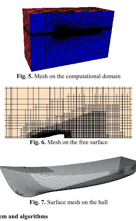
3.3 Mesh generation

Fig. 5. Mesh on the computational domain

Fig. 6. Mesh on the free surface

Fig. 7. Surface mesh on the hull

4. Optimisation problem and algorithms

A general constrained optimisation problem can be defined as follows: Minimize f(X)

Subject to u≤Xk_{≤v; k=1,2,…,p} gj(X)=0; j=1,2,…,q

hj(X)≥0; j= 1,2,…,r （1） where f is the objective function, X=[ x1, x2,…, xn]T represents the n-dimensional vector of the design variables, Xk _{denotes a set of k-th design variable, u=[ u}

1, u2,…, un]T and v=[ v1, v2,…, vn]T are the minimum and maximum bounds for the n-dimensional vector of the design variables, respectively, q is the number of the equality constraints, and r is the number of the inequality constraints.

4.1 Non-linear programming by quadratic Lagrangian (NLPQL)

The gradient algorithm can find the optimal solution step by step according to the direction Sk and the step length ɑk_{. After giving an initial point X}0_{, the algorithm will find a new point X}1_{in order} to decrease the object function value f. This step is repeated until the optimisation problem gets its optimal solution X*. X is updated by using:

non-linear constraints and the next design point can be obtained by solving the quadratic programming. Then, a linear search is performed according to two alternative optimisation functions. In this algorithm, the Hessian matrix is updated by using the Broyden-Fletcher-Goldfarb-Shanno (BFGS) algorithm. The algorithm is designed to solve the constrained nonlinear programming problem by generating a sequence of iterates, X, whereby an approximation is minimized at each iteration (Van and Koch, 2010).

4.2 Design of experiments (DoE)

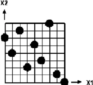
The DoE approach is a statistical method that enables appropriate data to be designed and analysed to extract the process characteristics for a fixed space with fewer simulation runs. Due to the weakness of the gradient optimisation method as explained above, the initial design point is generated using the DoE method. In recent years, many DoE methods have been proposed, such as Full Factorial Design (FFD), Orthogonal Arrays (OA) and Latin Hypercube Design (LHD). Compared with the FFD technique, shorter experiment times can be obtained for each factor for the LHD technique (Lai, 2012). ISIGHT (2014) assumed that an advantage of the LHD technique over the OA technique is that more points and more combinations can be studied for each factor. Therefore, the LHD technique was used to obtain an optimal solution in the hull form optimisation space. In the LHD algorithm, the design space for each factor is divided uniformly (the same number of divisions, n, for all factors). These levels are randomly combined to specify n points defining the matrix design (each level of a factor is studied only once) (ISIGHT, 2014). For a three levels of three factors problem, Fig. 8 shows the configuration of 9 points studied using the LHD technique.

Fig. 8. Samples designed using the LHD technique (ISIGHT, 2014)

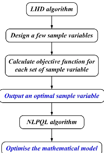
4.3A hybrid algorithm

A hybrid algorithm is developed in this study to solve the non-linear mathematical optimisation problem, integrating a LHD technique and a NLPQL algorithm. The flow chat of this algorithm can be found in Fig. 9 which is also summarised as follows:

1. A LHD algorithm is employed to design a few sample variables in an optimisation space. 2. An evaluation method is used to calculate the objective function values using these sample variables.

3. The objective function values are compared for different sample variables, and an optimal sample variable is obtained.

Fig. 9. Flow chart of a hybrid algorithm

4.4Validation of the efficiency of the hybrid algorithm

Two test functions are used to validate the efficiency of the hybrid algorithm. The first function is a Shubert function (f1(x)), and the second one is Schaffer function (f2(x)). These two equations are given in Equations (3) and (4) as follows:









































1

(

)

*

cos[(

1

)

*

]

*

cos[(

1

)

*

]

i

x

i

i

i

x

i

i

x

f

2 2 2 2 1 2 2 2 1 2 2

))

(

001

.

0

1

(

5

.

0

))

(sin(

cos

5

.

0

)

(

x

x

x

x

x

f













A single NLPQL algorithm and a hybrid algorithm are employed to find the minimum values of these two equations, respectively. As shown in Section 4.3, the first step of the hybrid algorithm is to use the LHD algorithm to find some sample variables in the optimisation space. We therefore used the LHD algorithm to design 20 sample variables for each equation. As the LHD technique is a random algorithm, three sets of samples are designed, as shown from Table 2 to Table 4. The parameters x1 and

x2 in Table 2 to Table 4 are the corresponding variables in Equations (3) and (4), respectively, obtained by LHD algorithm. f1(x) and f2(x) are the results calculated using Equations (3) and (4), respectively (see Tables, 2, 3 and 4).

Table 2 First samples

No. _x1 LHD for _x2 f1(x) _{f1(x) x1} LHD for _x2 f2(x) _f2(x)

1 -10 8.95 0.4758 -100 5.263 0.500091

2 -8.95 -8.95 3.419718 -89.474 -15.789 0.504920

3 -7.89 4.74 88.8806 -78.947 100 0.500715

4 -6.84 -6.84 35.7938 -68.421 -47.368 0.507509

5 -5.79 1.58 -0.47231 -57.895 57.895 0.508425

6 -4.74 5.79 0.911826 -47.368 15.789 0.524917

7 -3.68 7.89 0.650729 -36.842 -57.895 0.510652

8 -2.63 -0.53 -11.08 -26.316 -89.474 0.502565

9 -1.58 -4.74 -3.95412 -15.789 68.421 0.505087

10 -0.53 6.84 1.768221 -5.263 36.842 0.519360

11 0.53 0.53 1.101619 5.263 -5.263 0.948887

12 1.58 10 0.835354 15.789 -100 0.500557

13 2.63 -2.63 3.346347 26.316 -36.842 0.483858

14 3.68 -1.58 27.57458 36.842 -78.947 0.504314

15 4.74 -3.68 9.652096 47.368 89.474 0.503677

16 5.79 2.63 -2.87314 57.895 47.368 0.500357

17 6.84 -7.89 -3.3225 68.421 26.316 0.499730

18 7.89 3.68 2.131568 78.947 -26.316 0.496762

19 8.95 -5.79 -3.48161 89.474 -68.421 0.502039

20 10 -10 0.863757 100 78.947 0.500715

Table 3 Second samples

No. _x1 LHD for _x2 f1(x) _{f1(x) x1} LHD for _x2 f2(x) _f2(x)

1 -10 -3.68 0.231251 -100 -100 0.501134

2 -8.95 0.53 -1.94093 -89.474 -5.263 0.497625

3 -7.89 3.68 24.16905 -78.947 47.368 0.499878

4 -6.84 1.58 -1.49479 -68.421 -68.421 0.504656

5 -5.79 -6.84 11.30985 -57.895 100 0.501186

6 -4.74 -2.63 -1.062 -47.368 36.842 0.514729

7 -3.68 8.95 1.648599 -36.842 -26.316 0.483858

8 -2.63 2.63 3.346347 -26.316 -89.474 0.502565

9 -1.58 -8.95 17.39071 -15.789 78.947 0.496527

10 -0.53 -1.58 -41.254 -5.263 15.789 0.375849

11 0.53 4.74 -11.3175 5.263 -15.789 0.375849

12 1.58 -10 0.064546 15.789 26.316 0.613553

13 2.63 10 4.42964 26.316 89.474 0.502565

14 3.68 5.79 -6.35873 36.842 5.263 0.519360

15 4.74 -5.79 -20.3839 47.368 57.895 0.500357

16 5.79 -0.53 9.513228 57.895 -78.947 0.504447

17 6.84 -4.74 0.169481 68.421 -57.895 0.501631

18 7.89 -7.89 5.992185 78.947 -47.368 0.499878

19 8.95 6.84 -0.74237 89.474 -36.842 0.501617

Table 4 Third samples

No. _x1 LHD for _x2 f1(x) _{f1(x) x1} LHD for _x2 f2(x) _f2(x)

1 -10 -6.84 -1.54561 -100 -89.474 0.500779

2 -8.95 3.68 5.422279 -89.474 36.842 0.501617

3 -7.89 4.74 88.8806 -78.947 -36.842 0.504314

4 -6.84 8.95 -11.0187 -68.421 -100 0.501944

5 -5.79 -1.58 -17.7777 -57.895 78.947 0.504447

6 -4.74 5.79 0.911826 -47.368 -57.895 0.500357

7 -3.68 -3.68 0.801263 -36.842 15.789 0.496587

8 -2.63 1.58 0.631063 -26.316 68.421 0.499730

9 -1.58 -8.95 17.39071 -15.789 -78.947 0.496527

10 -0.53 0.53 4.604259 -5.263 -47.368 0.486319

11 0.53 -7.89 -8.65144 5.263 57.895 0.520877

12 1.58 -0.53 -1.09602 15.789 -68.421 0.505087

13 2.63 -5.79 -2.50453 26.316 26.316 0.587896

14 3.68 -2.63 7.406008 36.842 5.263 0.519360

15 4.74 2.63 14.2859 47.368 -15.789 0.524917

16 5.79 6.84 0.874131 57.895 100 0.501186

17 6.84 -10 -0.10413 68.421 89.474 0.502039

18 7.89 10 2.430566 78.947 -5.263 0.508033

19 8.95 7.89 1.338875 89.474 47.368 0.503677

20 10 -4.74 -1.4058 100 -26.316 0.499329

Table 5 Optimal solutions by different algorithms for f1(x)

Theoretical

minimum NLPQL algorithm

LHD+NLPQL First

samples samples Second samples Third Optimal solution -186.7309 -0.00536 -48.506 -123.550 -47.248

Table 6 Optimal solutions by different algorithms for f2(x)

Theoretical

minimum NLPQL algorithm

LHD+NLPQL First

samples samples Second samples Third

Optimal solution 0.292579 0.4974 0.47395 0.37328 0.48292

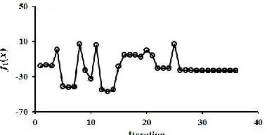
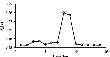
Fig. 11. Evolution history using NLPQL algorithm for f2(x)

Fig. 12. Evolution history using first samples by LHD+NLPQL algorithm for f1(x)

Fig. 13. Evolution history using second samples by LHD+NLPQL algorithm for f1(x)

Fig. 15. Evolution history using first samples by LHD+NLPQL algorithm for f2(x)

Fig. 16. Evolution history using second samples by LHD+NLPQL algorithm for f2(x)

Fig. 17. Evolution history using third samples by LHD+NLPQL algorithm for f2(x)

5. Optimisation strategy

5.1 Geometry regeneration

The ASD technique is a practical method to alter the shape of different geometries using the Sculptor software based on the B-spline technique. It can improve the geometric reconstruction efficiency with few design variables. In the optimum design, the geometry can be modified more freely, thus ensuring geometry smoothness. This technique therefore enables the optimisation of complex geometries (Sun et al., 2010). It has also been widely used in different optimisation problems (Lee et al., 2011; Li et al., 2016; Sun et al., 2010).

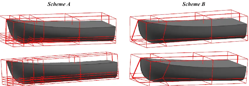
Fig. 18. The ASD volume around the original hull form with two different sets of design variables

Fig. 19. Four different examples of the geometry regeneration for the fishing boat

5.2 Optimisation procedure

To find an optimal global region of the research space, a Design of Experiment (DoE) method was employed to design some sampling hull forms before the optimisation in order to find an optimal global region. Following this, a NLPQL algorithm was used to find a global optimum value. Fig. 20 shows an overview of the optimisation design process. The essential steps can be summarised as follows:

1. Discretise the continuous research space using the LHD technique and obtain an optimal global region.

2. Define the initial design variable of the NLPQL algorithm. 3. Output a set of design variables.

4. Change the shape of the bow using the different design variables. 5. Build the new hull form and computational domain.

6. Mesh the computational domain.

7. Define the physical parameters of a new hull form, including the draft, the centre of mass, and the moment of inertia.

8. Simulate ship motions and calculate the total resistance coefficient.

Fig. 20. Flow chart for the hull form optimisation platform developed in this study

6. Optimisation

6.1 Optimisation problem

The optimisation objective is to find the optimal hull form with a minimum total resistance Rt (expressed using the total resistance coefficient Ct below) at the design speed of Fr=0.59. The draft of the modified hull form will be changed to maintain the same displacement as the original hull. Two sets of design variables, Scheme A and Scheme B, were used in this study. For the Scheme A, the bow was optimized by four design variables (a1, a2, a3, a4). a1, a2, a3 and a4 are moved along the y-direction, as shown in Fig. 18. For Scheme B, the bow geometry was changed by two design variables (b1, b2).

b1 is moved along the x-direction, and b2 is moved along the y-direction, as shown in Fig. 18. The range of these design variables can be summarized as follows:

-0.5≤a1≤0.5 （5）

-0.5≤a2≤0.5 （6）

-0.5≤a3≤0.5 （7）

-0.5≤a4≤0.5 （8）

-0.4≤b1≤0.4 （9）

-1≤b2≤0.5 （10）

As described above, the total resistance coefficient Ct is employed to express the total resistance Rt of a ship, and Ct can be defined as:

S

U

R

C

t



₀

_.

₅

_

where Rt is the total resistance of a ship, ρ is the fluid density, U is the speed of a ship, and S is the wetted surface area.

6.3 Results and discussion

6.3.1 Verification study

A verification study was undertaken to estimate the discretisation errors for the current CFD model for the resistance simulation at design speed. It is assumed that the numerical uncertainty δSN consists of the grid-spacing convergence error δG, time-step convergence error δT and iterative convergence error δI, as shown below:

δSN =δT+ δG + δI （12） For the grid-spacing convergence error δG and time-step convergence error δT, the uncertainty is predicted using Roache's (1998) grid convergence index (GCI) method, which was presented by Celik et al. (2008). This is a very useful method to estimate the uncertainties arising from grid-spacing and time-step errors (Kavli et al., 2017). Firstly, the convergence ratio Rk can be obtained by:

32 21 k k k

R







where εk21=φk2-φk1, and εG32=φk3-φk2. φk1, φk2, and φk3 represent the solutions calculated by fine, medium, and coarse mesh configurations. The subscript k refers to the k-th input parameter (i.e. grid-size or time-step) (Stern et al., 2006).

The convergence conditions are summarized as follows: (I) If 0<RG<1, the result is monotonic convergence; (Ⅱ) If Rk<0 and |Rk|<1, the result is oscillatory convergence; (Ⅲ) If Rk>1, the result is monotonic divergence; (Ⅳ) If Rk<0 and|Rk|>1, the result is oscillatory divergence. Stern et al. (2006) noted that the error and the uncertainty could not be assessed if the result is the condition (Ⅲ) or condition (Ⅳ).

The order-of-accuracy Pk is calculated by the generalized Richardson extrapolation method:

k k k k

r

P

ln

)

/

ln(







where rk is the constant refinement ratio.

The extrapolated values can be calculated from Celik et al. (2008):

)

1

(

)

(

21







r

r







The approximate relative error ea21 and extrapolated relative error eext21 can then be calculated as (Celik et al., 2008):

1 2 1 21











e

12 1 12 21 ext ext ext

e











1

25

.

1

21





k a fine

r

e

GCI

A constant refinement ratio of √2 was chosen to assess the convergence of the grid-spacing and time-step as used by many researchers recently (e.g. Owen et al. (2018), Sezen et al. (2018), Demirel et al. (2017), Mizzi et al. (2017)). Table 7 shows the final mesh numbers for each mesh configuration.

Table 7 Mesh configurations of the current CFD model for this mesh convergence study

Mesh configurations Cell numbers

Coarse 690525

Medium 1264198

Fine 2188115

For the iterative convergence error δI, the value is assessed using the method of Zhang et al. (2008), which results in the 0.305% Ct iterative error for the fine mesh.

Then grid-spacing and time-step convergence studies were carried out by using the method of Celik et al. (2008) as described earlier, and the verification parameters of the total resistance coefficient are presented in Table 8. As can be seen from Table 8, the total resistance coefficient results tend to monotonic convergence as both of the convergence ratio R are greater than 0 and less than 1. The numerical uncertainties in the fine mesh solution for grid-spacing and time-step convergence tests are predicted as 1.5418% and 0.0090965%, respectively. It can be pointed out that the grid-spacing is more sensitive than the time-step. Fig. 21 shows the Wall Y+ values on the ship hull at design speed.

Table 8 Grid-spacing and time-space convergence studies for the total resistance coefficient Ct

Items _{(with monotonic convergence)} Grid convergence _{(with monotonic convergence)} Time-step convergence

r √2 √2

φ1 0.027426 0.027426

φ2 0.027788 0.027446

φ3 0.028537 0.02767

R 0.48318 0.09009

p 2.0988 6.945

φ2ext21 0.027088 0.027424

ea21 1.3193% 0.0735%

eext21 1.2488% 0.0072777%

GCIfine21 1.5418% 0.0090965%

Fig. 21. The Wall Y+ values on the ship hull

6.3.2 Selection of the sample hull forms

Table 9 (a1, a2, a3 and a4) and Table 10 (b1 and b2). Following this, the CFD model presented above was used to calculate the total resistance coefficients for 20 hulls at design speed. Table 9 and Table 10 also show the total resistance coefficients of 20 hulls with corresponding sample variables and drafts designed. Bold values in the tables signify the optimal sample variable for each scheme. Following this, the optimal sample variable No.3 for Scheme A and No.20 for Scheme B were selected as the initial design variable of the NLPQL algorithm, and the optimisation results and discussion were presented in Section 6.3.3.

Table 9 Values obtained using the LHD technique for Scheme A

No. a1 a2 a3 a4 Draft (m) Ct

1 -0.5 0.5 -0.447 0.289 0.351185 0.027212

2 -0.447 0.447 -0.184 -0.237 0.35719 0.027256

3 -0.395 -0.079 -0.342 -0.184 0.36136 0.026896

4 -0.342 0.237 0.132 0.447 0.34023 0.02826

5 -0.289 0.395 0.447 0.395 0.33558 0.028432

6 -0.237 0.132 0.026 0.237 0.345705 0.02758

7 -0.184 0.289 -0.289 -0.395 0.36138 0.028024

8 -0.132 -0.132 0.395 -0.132 0.34785 0.027436

9 -0.079 -0.5 0.237 0.132 0.34702 0.027488

10 -0.026 -0.395 -0.237 -0.342 0.3625 0.027052

11 0.026 -0.342 0.184 0.184 0.3456 0.028116

12 0.079 -0.447 -0.079 -0.447 0.36175 0.027396

13 0.132 0.026 -0.132 0.5 0.3416 0.027788

14 0.184 -0.289 -0.5 0.342 0.352 0.027308

15 0.237 -0.184 0.079 -0.079 0.35021 0.027708

16 0.289 -0.237 -0.026 0.026 0.3497 0.027568

17 0.342 0.079 0.342 -0.289 0.3476 0.028076

18 0.395 0.184 0.289 0.079 0.34165 0.028496

19 0.447 -0.026 0.5 -0.026 0.34137 0.02746

Table 10 Values obtained using the LHD technique for Scheme B

No. b1 b2 Draft (m) Ct

1 -0.4 0.263 0.34713 0.029508

2 -0.358 0.421 0.34416 0.028812

3 -0.316 -0.842 0.36855 0.027872

4 -0.274 -0.053 0.3523 0.028508

5 -0.232 0.026 0.3505 0.028588

6 -0.189 -0.921 0.3697 0.02748

7 -0.147 -0.211 0.3546 0.027968

8 -0.105 0.342 0.3442 0.02872

9 -0.063 0.5 0.3415 0.0289

10 -0.021 -0.132 0.3524 0.0275

11 0.021 0.105 0.3478 0.027492

12 0.063 -0.289 0.3552 0.027068

13 0.105 0.184 0.3458 0.02754

14 0.147 -0.605 0.3613 0.026736

15 0.189 -0.368 0.3561 0.026692

16 0.232 -1 0.3696 0.026256

17 0.274 -0.763 0.3641 0.026248

18 0.316 -0.447 0.3568 0.026416

19 0.358 -0.526 0.3586 0.025984

20 0.4 -0.684 0.3617 0.025868

6.3.3 Analysis between original and optimal hull forms

The optimisation framework was carried out on an Intel Core i5-5200U CPU @2.2 GHz, and the CFD runs in this paper were performed using the ARCHIE-WeST High Performance Computer (http://www.archie-west.ac.uk). Each generation was computed for approximately 400 CPU hours. With a supercomputer, each simulation can be completed in a couple of days. After the optimisation, two optimal hull forms were obtained using different design variables, and the optimum results can be found in Table 11.

Table 11 The optimisation results for each method at the design speed

New draft Resistance reduction %

opt org

Sinkage

Sinkage

opt org

Trim

Trim

Scheme A 0.3676 3.89 1.0162 1.2537

Scheme B 0.3617 5.70 1.0067 1.0924

As can be seen from Table 11, the optimisation loop achieves a total resistance reduction of 3.89% and 5.70% at the design speed using Scheme A and Scheme B, respectively. The trim is the main factor influencing the total resistance of the fishing boat, since it significantly changes the underwater shape of the boat in calm water. Compared to the original hull form, the sinkage and trim of the optimal hull form was reduced by 1.59% and 20.24% for Scheme A, and was decreased by 0.66% and 8.45% for Scheme B. It can be concluded that the sinkage and trim of the optimal hull can also improve a ship’s stability and safety, and this optimisation loop is a promising method to design new hull forms for reducing not only the total resistance but also the sinkage and trim.

12.

(a) Scheme A (b) Scheme B

Fig. 22. Evolution history for two optimisations (Scheme A and Scheme B)

Table 12 The optimal solutions obtained using the hybrid algorithm for the two optimisations employed

Scheme A Scheme B

a1 a2 a3 a4 b1 b2

-0.5 0.49999 -0.5 -0.499 0.399 -0.684

Since the optimisation was only carried out at design speed, further calculations were performed to predict the total resistance coefficients at different Fr values to calculate the drag reduction for the optimal hulls. Table 13 shows the comparison of the total resistance coefficients between the original and the optimal hull forms obtained through the optimisation using Schemes A and B, individually. When comparing the efficiency of the schemes employed in the optimisation process, it is clear from Table 13 that Scheme B gives a larger reduction in total resistance for each Froude number than Scheme A. The reduction in the total resistance of the optimized hull form using Scheme B is more pronounced for lower Froude numbers. Another interesting result which can be drawn from Table 13 is that Scheme A gives the largest percentage reduction (3.89%) at the design speed. It should however be noted that for Froude number 0.4, Scheme A gives an increase in the total resistance of the optimized hull compared to the original hull, rather than an expected reduction. For this reason, it can be concluded that Scheme A may not be appropriate to be used for optimisation for lower Froude number ranges.

Fig. 23 presents the body-plans for the original and optimal hulls. The bow contour line of the optimal hull form was not changed much for Scheme A, while it changes more significantly for Scheme B due to the change in design variable b1. It can be interpreted from Fig. 23 that a suitable bow contour line is more beneficial to reduce the total resistance for a fishing boat, as also shown in Table 13.

Table 13 A comparison of the total resistance coefficients for the original and optimal hulls

Fr Original hull _C Optimal hull for Scheme A Optimal hull for Scheme B

t Ct Reduction (%) Ct Reduction (%)

0.4 0.016272 0.01798 -10.50 0.015112 7.13

0.5 0.022388 0.022112 1.23 0.020816 7.02

0.59 0.027426 0.026359 3.89 0.025862 5.70

0.6 0.02687 0.02623 2.38 0.025364 5.60

0.7 0.02136 0.020964 1.85 0.020596 3.58

(a) Scheme A

(b) Scheme B

Fig. 23. A comparison of the geometry for the original hull and the optimal hulls

Fig. 24 and Fig. 25 present a comparison of the wave patterns and wall shear stress on the hull surface for the original and optimal hull forms, respectively. As can be seen from Fig. 24, the bow waves of the optimized hull forms are reduced compared with the original hull, and the shoulder waves and stern waves are also reduced or cancelled for the optimal hull forms. All of these physical phenomena illustrate why the total resistance of the optimal hull forms has been reduced. The wall shear stress distribution of the bow section undergoes a significant change for the optimal hull forms, especially near the bow contour line, as shown in Fig. 25.

(b) Scheme B

Fig. 24. Comparison of the wave patterns

Fig. 25. Comparison of the wall shear stress on the hull surface

7. Conclusions and future work

By changing the shape of the bow of a fishing boat, a practical ship hull form optimisation framework was presented in this study for reducing the total resistance in calm water at the design speed (Fr=0.59), using a hybrid algorithm.

time-space convergence studies for the total resistance coefficient tend to monotonic convergence. Next, a hybrid algorithm was developed, and its detail was presented including the LHD technique and NLPQL algorithm. Following this, a geometry regeneration method was listed to alter the shape of the bow with four and two design variables, respectively. Then, four examples of possible deformations of the fishing boat were shown to illustrate the practicability of the ASD technique. It was demonstrated that a new fishing boat geometry can be obtained using the ASD technique in less than one minute with few variables, improving the optimisation efficiency.

The optimisation framework in this study was then carried out for a single velocity with a single objective. After the completion of the optimisation, two optimal hulls were obtained. Then, the total resistance, sinkage, trim, and flow field were compared for the original hull and the optimal hulls. The optimisation loop achieved a total resistance reduction of 3.89% and 5.70% for Scheme A and Scheme B, respectively. It can be concluded that a suitable bow contour line is more beneficial to reduce the total resistance for a fishing boat. The bow waves, shoulder waves, stern waves and the wall shear stress on the hull surface of the optimized hull forms were reduced or cancelled compared with the original hull. The sinkage and trim of the optimal hull form were reduced by 1.59% and 20.24% for Scheme A, and they were decreased by 0.66% and 8.45% for Scheme B. This indicates that the trim is more sensitive than the sinkage for new hull forms. The optimisation results show that the optimisation framework developed in this paper can be used to optimise the fishing boat, which can also provide technical support and a theoretical basis for designing green ships.

As the performance of the fishing boat in waves is different from its behaviour in calm water, further studies will focus on the ship hull form design optimisation in waves. A total resistance of a fishing boat in waves will be used as the objective function, and an optimal ship hull form will be obtained to meet the actual navigation condition.

Acknowledgements

This research project is funded by the Institutional Links Grants (Grant ID: 217539254) of the British Council. The authors would like to thank the valuable discussions and suggestions provided by Dr Setyo Nugroho, Dr Heri Supomo, Mr Imam Baihaqi and Dr Zhiming Yuan. The authors would like to thank Dr Holly Yu for her help with the final proofreading. CFD results were obtained using the EPSRC funded ARCHIE-WeST High Performance Computer (www.archie-west.ac.uk). EPSRC grant no. EP/K000586/1.

Reference

Ahmed, Y.M. 2011. Numerical simulation for the free surface flow around a complex ship hull form at different Froud numbers. Alexandria Engineering Journal, 50(3): 229-235.

Attaviriyanupap, P., Kita, H., Tanaka, E., Hasegawa, J., 2002. A hybrid EP and SQP for dynamic economic dispatch with nonsmooth fuel cost function. IEEE Transactions on Power Systems 17 (2), 411-416.

Azimifar, A., Payan, S., 2016. Enhancement of heat transfer of confined enclosures with free convection using blocks with PSO algorithm. Applied Thermal Engineering 101, 79-91.

Bagheri, H., Ghassemi, H., 2014. Genetic algorithm applied to optimization of the ship hull form with respect to seakeeping performance. Transactions of Famena 38 (3), 45-58.

Barroso, E.S., Jr, E.P., Melo, A.M.C. 2017. A hybrid PSO-GA algorithm for optimization of laminated composites. Struct Multidisc Optim, 55:2111-2130.

Carrica, P.M., Huiping, F., Stern, F. 2011. Computations of self-propulsion free to sink and trim and of motions in head waves of the KRISO container ship (KCS) model. Appl. Ocean Res. 33 (4), 309-320.

CD-Adapco, 2014. User guide STAR-CCM+ Version 9.0.2.

Celik, I.B., Ghia, U., Roache, P.J., Freitas, C.J., 2008. Procedure for estimation and reporting of uncertainty due to discretization in CFD applications. J. Fluids Eng. Trans. ASME 130 (7), 078001.

Chen, S.T., Zhong, J.J., Sun, P. 2015. Numerical simulation of the Stokes wave for the flow around a ship hull coupled with the VOF model. J. Marine Sci. Appl. 14: 163-169.

Date, J.C., Turnock, S.R., 1999. A study into the techniques needed to accurately predict skin friction using RANS solvers with validation against Froude’s historical flat plate experimental data. University of Southampton, Southampton, UK p. 62 (Ship Science Reports, (114)).

Demirel, Y.K., Turan, O., Incecik, A., 2017. Predicting the effect of biofouling on ship resistance using CFD. Applied Ocean Research 62, 100-118. http://dx.doi.org/10.1016/j.apor.2016.12.003

Gammon, M.A., 2011. Optimization of fishing vessels using a multi-objective genetic algorithm. Ocean Engineering 38 (10), 1054-1064.

Garg, H., 2016. A hybrid PSO-GA algorithm for constrained optimization problems. Applied Mathematics & Computation 274 (11), 292-305.

Gill, P.E., Murray, W., Saunders, M.A., 2002. SNOPT: An SQP Algorithm for Large-Scale Constrained Optimization. Siam Journal on Optimization 12 (4), 979-1006.

Hirt, C. W., Nichols, B., 1981. Volume of fluid method for the dynamics of free boundaries. Comp. Phys, 39(1): 20-225.

ISIGHT, 2014. User guide ISIGHT Version 5.9.

International Towing Tank Conference (ITTC). 2014. Practical guidelines for ship resistance CFD. https://ittc.info/media/4198/75-03-02-04.pdf

Kavli, H.P., Oguz, E., Tezdogan, T., 2017. A comparative study on the design of an environmentally friendly RoPax ferry using CFD. Ocean Engineering, 137: 22-37. doi.org/10.1016/j.oceaneng.2017.03.043.

Lee, Y.T., Ahuja, V., Hosangadi, A., Slipper, M.E., Mulvihill, L.P.., Birkberk, R., Coleman, R.M., 2011. Impeller design of a centrifugal fan with blade optimization. International Journal of Rotating Machinery, 1-16.

Lai, Y.Y. 2012. ISIGHT parameter optimization and the detailed solutions. Beijing, China. Beijing University of Aeronautics and Astronautics Press.

Li, H.Y., Wen, Y.G., He, H.Z., Li, B.L. 2014. An image segmentation algorithm based on random weight particle swarm optimization and K-means clustering. Journal of Graphics, 35(5): 755-761. Li, R., Xu, P., Peng, Y., Ji, P., 2016. Multi-objective optimization of a high-speed train head based on

the FFD method. Journal of Wind Engineering and Industrial Aerodynamics 152, 41-49.

Li, S.Z. 2012. Research on hull form design optimization based on SBD technique. China Ship Scientific Research Center, Beijing.

Lowe, T.W., Steel, J., 2003. Conceptual hull design using a genetic algorithm. Journal of Ship Research 47 (3), 222-236.

Mizzi, K., Demirel, Y.K., Banks, C., Turan, O., Kaklis, P., Atlar, M., 2017. Design optimisation of Propeller Boss Cap Fins for enhanced propeller performance. Applied Ocean Research 62, 210-222. http://dx.doi.org/10.1016/j.apor.2016.12.006.

Owen, D., Demirel, Y.K., Oguz, E., Tezdogan, T., Incecik, A., 2018. Investigating the effect of biofouling on propeller characteristics using CFD. Ocean Engineering 159, 505-516. http://dx.doi.org/10.1016/j.oceaneng.2018.01.087

Park, J.H., Choi, J.E., Chun, H.H. 2015. Hull-form optimization of KSUEZMAX to enhance resistance performance. International Journal of Naval Architecture & Ocean Engineering, 7(1): 100-114.

Patankar, S.V., Spalding, D.B., 1972. A calculation procedure for heat, mass and momentum transfer in three-dimensional parabolic flows. International Journal of Heat and Mass Transfer 5 (15), 1787-1806.

Peri, D. 2016. Robust Design Optimization for the refit of a cargo ship using real seagoing data. Ocean Engineering, 123:103-115.

Roache, P.J., 1998. Verification and Validation in Computational Science and Engineering. Hermosa Publishers, Albuquerque.

Saha, G.K., Miazee, M.A. 2017. Numerical and experimental study of resistance, sinkage and trim of a container ship. Procedia Engineering, 194: 67-73.

SIGGRAPH computer graphics, 20(4):151-160.

Serani, A., Fasano, G., Liuzzi, G., Lucidi, S., Iemma, U., Campana, E.F., Stern, F., Diez, M. 2016. Ship hydrodynamic optimization by local hybridization of deterministic derivative-free global algorithms. Applied Ocean Research, 59:115-128.

Sezen, S., Dogrul, A., Delen, C., Bal, S., 2018. Investigation of self-propulsion of DARPA Suboff by RANS method. Ocean Engineering 150, 258-271.

Stern, F., Wilson, R., Shao, J., 2006. Quantitative V & V of CFD simulations and certification of CFD codes. Int. J. Numer. Methods Fluids 50 (11), 1335-1355.

Sun, Z.X., Song, J.J., An, Y.R., 2010. Optimization of the head shape of the CRH3 high speed train. Science China of Technological Sciences 53, 3356-3364.

Tezdogan, T., Incecik, A., Turan, O. 2016. Full-scale unsteady RANS simulations of vertical ship motions in shallow water. Ocean Engineering, 123:131-145.

Tungadio, D.H., Jordaan, J.A., Siti, M.W., 2016. Power system state estimation solution using modified models of PSO algorithm: Comparative study. Measurement 92, 508-523.

Van, A., Koch, P. 2010. Isight Design Optimization Methodologies. Isight Design Optimization Methodologies, ASM Handbook Volume 22B Application of Metal Processing Simulation. Wang, S., Su, Y.M., Pang, Y.J., Liu, H.X., 2014. Numerical study on longitudinal motions of a

high-speed planing craft in regular waves. Journal of Harbin Engineering University 35 (1), 45-52.

Wu, J.W., Liu, X.Y., Zhao, M., Wan, D.C. 2017. Neumann-Michell theory-based multi-objective optimization of hull form for a naval surface combatant. Applied Ocean Research, 63: 129-141. Yang, C., Huang, F.X. 2016. An overview of simulation-based hydrodynamic design of ship hull

forms. Journal of Hydrodynamics, 28 (6): 947-960.

Yousefi, R., Shafaghat, R., Shakeri, M., 2014. High-speed planing hull drag reduction using tunnels. Ocean Engineering 84, 54-60.

Yu, J.M., Lee, Y.G., 2016. Hull form design for the fore-body of medium-sized passenger ship with gooseneck bulb. International Journal of Naval Architecture & Ocean Engineering 1-11.

Zha, R.S., Ye, H.X., Shen, Z.R., Wan, D.C. 2014. Numerical computations of resistance of high speed catamaran in calm water. Journal of Hydrodynamics, 26(6): 930-938.

Zhan, C.S., Liu, Z.Y., Feng, B.W., Chang, H.C. 2012. CFD-based automatical optimization of bulbous bow lines. Journal of Ship Mechanics, l6(4): 351-358.

Zhang, N., Shen, H.C., Yao, H.Z. 2008. Uncertainty analysis in CFD for resistance and flow field. Journal of Ship Mechanics, 12(2): 211-224.

Zhang, B.J., Ma, K., Ji, Z.S., 2009. Optimization Design of the Stem Shape for Full-Scale Ship Based on Nonlinear Programming Method. Shipbuilding of China 50 (2), 97-105.

Zhang, B.J., Ma, K., Ji, Z.S. 2011. Optimization design for hull form of minimum total resistance based on genetic algorithms. Journal of Ship Mechanics, l5(4): 325-331.

Zhang, B.J., 2012. Optimization design of hull lines based on hybrid optimization algorithm. Journal of Shanghai Jiaotong University 46 (8), 1238-1242.

Zhang, B.J., Zhang, Z.X. 2015. Research on theoretical optimization and experimental verification of minimum resistance hull form based on Rankine source method. International Journal of Naval Architecture & Ocean Engineering, 7(5): 785-794.

Zhang, S.L., Zhang, B.J., Tezdogan, T., Xu, L.P., Lai, Y.Y. 2017. Research on bulbous bow optimisation based on the improved PSO algorithm. China Ocean Engineering, 33(4): 487-494. Zhu, L.M., Zhao, L. 2017. Research on mobile robot path planning by using improved genetic