Noise coupling effect in multi-antenna systems

Noise Coupling Effect in

M ulti-antenna Systems

Snezana Krusevac

November 2007

A thesis submitted for the degree of Doctor of Philosophy of the Australian National University

Declaration

i

The contents of these thesis are the results of original research and have not been submitted for a higher degree to any other university or institution.

Much of the work in this thesis has been published or has been submitted for publication as journal paper or conference paper. These papers are:

1. S. Krusevac, P. B. Rapajic and R. A. Kennedy, Mutual Coupling Effect on Thermal Noise in Multi-antenna Communication System, Progress in Electromagnetics Research (PIER) Journal PIER 59, pages 325-333, 2006.

2. S. M. Krusevac, P. B. Rapajic and R. A. Kennedy, Thermal Noise Mutual Coupling Effect on the Capacity of MIMO Wireless Systems, Wireless Personal Communications Journal, Springer, volume 40 (3), pages 317-328, Feb. 2007.

3. S. Krusevac, P. B. Rapajic and R. A. Kennedy, Method for MIMO Channel Capacity Estimation for Electro-Magnetically Coupled Transmit Antenna Elements, Proc. 5th Australian Communications Theory Workshop, AusCTW’2004, pages 122-126, Newcastle,

Australia, Feb. 2004.

4. S. Krusevac, P. B. Rapajic and R. A. Kennedy, Channel Information Capacity for Mutually Coupled Transmittal Antennas, Proc. 2004 Progress in Electromagnetics Research Symposium, PIERS 2004, pages 639-642, Pisa, Italy, Mar. 2004.

5. S. Krusevac, P. B. Rapajic and R. A. Kennedy, The Method for MIMO Channel Capacity Estimation in the Presence of Spatially Correlated Noise, Proc. 2004 IEEE International Symposium on Spread Spectrum Techniques and Applications, ISSSTA 2004, pages 511-514, Sydney, Australia, Sep. 2004.

ii

Systems, Proc. 6th Australian Communications Theory Workshop, AusCTW’2005, pages 192-197, Brisbane, Queensland, Australia, Feb. 2005

7. S. Krusevac, P. B. Rapajic and R. A. Kennedy, Capacity Bound of MIMO Systems in the Presence of Spatially Correlated Noise, Proc. 8th International Symposium on Communication Theory and

Applications, ISCTA05, pages 298-303, Ambleside, Lake District, UK, July 2005.

8. S. Krusevac, P. B. Rapajic and R. A. Kennedy, Effect of Mutual Coupling on the Performance of Multielement Antenna Systems, Proc. 2005 IEEE International Symposium on Antennas and Propagation, ISAP05, pages 565 - 568, Seoul, Korea, Aug. 2005. 9. S. Krusevac, P. B. Rapajic and R. A. Kennedy, Mutual Coupling

Effect on Thermal Noise in Multi-antenna Communication System, Proc. 2005 Progress in Electromagnetics Research Symposium, PIERS 2005, pages 53-57, Honzhou, China, Aug. 2005.

10. S. Krusevac, P. B. Rapajic and R. A. Kennedy, Channel Capacity of Multi-antenna Communication Systems with Closely Spaced Antenna Elements, Proc. The 16th Annual IEEE International Symposium on Personal Indoor and Mobile Radio Communications, IEEE PIMRC 2005, pages 2366-2370, Berlin, Germany, Sep. 2005.

11. S. Krusevac, P. B. Rapajic and R. A. Kennedy, Thermal Noise Mutual Coupling Effect on the Capacity of MIMO Wireless Systems, Proc. Wireless Personal Multimedia Communications Symposia 2005, WPMC’05, pages 466 - 470, Aalborg, Denmark, Sep. 2005.

i i i

13. S. Krusevac, P. B. Rapajic and R. A. Kennedy, Channel Capacity of MIMO Wireless Systems with Correlated Noise, Proc. 2005 IEEE Global Telecommunications Conference, IEEE GLOBECOM 2005, pages 2812-2816, St. Louis, Missouri, USA, Dec. 2005.

14. S. Krusevac, P. B. Rapajic, Channel Capacity of MIMO Systems with Closely Spaced Terminated Antennas , ISIT 2007, pages 1076-1080, 24 - 29 June 2007, Nice, France

The research represented in this thesis has been performed jointly with Professor Predrag B. Rapajic and Professor Rodney A. Kennedy. The substantial majority of this work is my own.

A ck n o w led g em en ts

I would like to extend my sincere thank to my supervisors Prof. Rodney A. Kennedy and Prof. Predrag B. Rapajic for letting me dictate the pace of my research, giving me freedom to a large extent on the choice of topics, their invaluable guidance and encouragement, and for giving me invaluable insight into my research.

I would also like to thank A. Prof. Thushara Abhayapala and A. Prof. Rodica Roamer for many fruitful discussions during my research. Although no results from these interactions become part of this thesis, the experience was invaluable and their energy and enthusiasm was infectious.

My friends and colleagues at the University of New South Wales, National ICT Australia and Australian National University, for providing fruitful and pleasant research environment.

I would like thank to my family and friends who make it all worth while. My mother Stojanka for believing in me (if I ever become as good as you believe in me - it will be purely a result of good genes). My sister Sladjana has supported me with her endless love, caring and patience. My dearest nephew Nikola and nice Hristina have enhanced my life in every respect. My brother-in-low Zvezdan for being friend out of ordinary.

Finally, no words are sufficient to express my love and gratitude to my husband Zarko and my baby daughter Nevena. Zarko has supported and encouraged me in pursuing my dreams, and has always been there to make sure they become realities. Nevena is the sunshine in my universe - each day is brighter because of her love and sweetness. I am incredibly lucky to share my life with these two special people.

A b s tr a c t

Close antenna spacing, less than a half of a wavelength, in multi-antenna systems results in mutual coupling which affects the capacity performance of multi-antenna systems. In contrast to previous studies which study mutual coupling’s effect on signals, this thesis examines the effect of mutual coupling on thermal noise.

We investigate noise correlation in closely spaced multiple antennas, and find that noise is correlated due to the mutual coupling. We calculate the noise covariance matrix, and the corresponding total thermal noise power in multi-antenna systems by applying the Nyquist thermal noise theorem. Then, we calculate the receive signal-to-noise ratio in the coupled antenna system to complete the quantitative analysis.

By taking into account the noise correlation effect, we provide an analysis of the ergodic channel capacity with equal power allocation and water-hlling power allocation schemes of the transmitted power. We show that ergodic capacity of MIMO systems is underestimated if the noise correlation due to the mutual coupling on thermal noise is neglected. Furthermore, we con­ firm that the water-filling allocation scheme is superior to the equal-power allocation scheme, which is more significant when multiple antennas with non-uniformly spaced antennas are used at the receiver. In that case the noise coupling affects the signal-to-noise ratio of individual antennas differ­ ently.

vi

of outage capacity when the mutual coupling on the noise is accounted for. We look at the effective degrees of freedom in the MIMO systems in order to isolate the noise correlation effect on the channel capacity. We show that for a very small antenna spacing (d — > 0), when the number of effective subchannels drops to 1, the water-filling allocation scheme is superior as it reconfigures to the optimal situation of allocating the total power to only one receiving antenna. We extract the contribution from the noise correlation in the channel capacity formula by deriving the noise correlation factor. It en­ ables us to derive of the upper bound on channel capacity of MIMO system in the presence of correlated noise. This is a significant result as it further enables us to estimate the channel capacity of the multiple antennas with closely spaced antennas avoiding complex matrix computations, which are time-consuming for large numbers of antenna elements. We conclude that noise coupling is a substantial parameter in determining the channel capacity of closely spaced multiple antennas.

In order to accurately calculate the received correlated noise power, we consider the antenna mismatching impedance effect. We analyze the noise covariance matrix for the three most common antenna terminated matching networks. We show that multi-port conjugate match acts not only as the optimal match in terms of maximal delivered signal power, but also as the whitening filter for the coupled thermal noise.

C o n te n ts

A c k n o w le d g e m e n ts iv

A b s tr a c t v

N o ta tio n a n d te r m in o lo g y x iii

I M u t u a l C o u p lin g in M u l t i - a n t e n n a S y s te m 1

1 I n tr o d u c tio n 2

1.1 Motivation and B ack g ro u n d ... 2

1.2 M u ltip le A n ten n as ... 4

1.3 Closely Spaced Multiple A ntennas... 9

1.3.1 Mutual Coupling Effect ... 9

1.3.2 Modeling of Closely Spaced Multiple A ntennas... 11

1.4 Summary of A p p ro a c h ... 15

1.5 Structure of this T hesis... 16

1.5.1 Questions to be Answered in this T h e s i s ... 16

1.5.2 Content and Contributions of T h e s i s ... 17

2 C o r re la te d N o ise 20 2.1 Introduction... 20

2.2 Antenna Noise... 21

2.2.1 Thermal Noise ... 22

2.3 Noise C o u p lin g ...24

2.3.1 Thermal Noise Electromagnetic R a d ia tio n ... 25

2.3.2 Nyquist Thermal Noise Theorem ... 25

CONTENTS viii

2.4 Noise in Multi-antenna S y s te m s ... 27

2.4.1 Two-antenna C a s e ... 27

2.4.2 General C a s e ...30

2.5 Noise Correlation Matrix - D efin itio n ... 31

2.6 Simulation E x p e rim e n ts ... 33

2.7 Summary and C ontributions... 36

3 S ig n a l-to -N o ise R a tio A n a ly sis 37 3.1 System O v erv iew ...37

3.1.1 Layered Space-time S tr u c tu r e ... 37

3.1.2 Receiving Unit ... 39

3.2 Coupling Effect on Average S N R ... 40

3.2.1 Signal Spatial C o rre la tio n ... 41

3.2.2 SNR A n a ly sis...43

3.3 Simulation R e s u l t s ...45

3.4 Summary and C ontributions... 48

4 C o n c lu sio n s an d F u tu re w ork 49 4.1 C onclusions... 49

4.2 Future Directions of R e s e a rc h ... 50

II M u ltip le A n te n n a C h a n n e l C a p a c ity 52 5 In tr o d u c tio n 53 5.1 Wireless Communication C h a n n e ls ... 53

5.2 Channel C ap acity ...56

5.2.1 Single Input Single Output (SISO) S y s te m ...58

5.3 MIMO Fading Channel Capacity ... 59

5.3.1 Erodic C apacity...59

5.3.2 Outage C a p a c ity ... 60

5.3.3 Channel Unknown at the T ransm itter...60

5.3.4 Channel Known at the T ra n sm itte r...62

5.4 Channel Modeling...63

CONTENTS ix

5.4.2 Spatial C o rrela tio n ... 63

5.4.3 Mutual Coupling Effect on Channel Matrix Coefficients 67 5.4.4 Content and Contributions of the Second Part of the T h e s is ... 68

6 C h a n n el C a p a c ity A n a ly sis 70 6.1 Introduction... 70

6.2 Ergodic MIMO Channel Capacity A nalysis... 72

6.2.1 Equal-power Allocation S c h e m e ... 72

6.2.2 Water-hlling Power Allocation S c h e m e ...74

6.2.3 Simulation R e s u l ts ... 76

6.3 Outage MIMO Channel Capacity A n a ly s is...80

6.4 Effective Degrees of Freedom ... 84

6.5 Noise Correlation F a c to r ...86

6.6 Summary and C ontributions... 90

7 T erm in a tio n d e p e n d a n c e 93 7.1 Introduction... 93

7.2 Matching Network Specification... 94

7.2.1 Characteristic Impedance M atch ...94

7.2.2 Self-Impedance M a t c h ... 95

7.2.3 Multiport Conjugate (MC) M a tc h ... 96

7.3 Noise Power A nalysis...97

7.4 Capacity A nalysis... 100

7.4.1 Simulation R e s u l ts ... 102

7.5 Summary and C ontributions...106

8 C o n clu sio n s an d F u tu re w ork 108 8.1 C onclusions... 108

8.2 Future Directions of R e s e a rc h ...110

L is t o f F ig u re s

1.1 Beamforming technique with two-antenna a r r a y ... 5

1.2 Beamforming technique with n-antenna a r r a y ... 6

1.3 Diversity combining tech n iq u e... 7

1.4 Spatial multiplexing technique... 8

1.5 Network representation of multi-antenna system with coupled a n te n n a s... 11

2.1 Equivalent representations of a resistance (at temperature T): (a) resistance represented as a noiseless resistance in series with a voltage source (b) resistance represented as a current source in parallel with a noiseless r e s is ta n c e ...23

2.2 (a) Two coupled antennas and corresponding representation of their self (Zn , Z22), mutual (Z12, Z2\) and load (Zli, Zl2) impedances (b) Network representation for two antenna array with voltage noise generators associated with antennas E\ , E2 and load El\ , El2 im pedances... 26

2.3 Block diagram of the receive subsystem including coupled an­ tenna array and lo ad s... 30

2.4 Effect of mutual coupling on average thermal noise power per antenna element in the multiple element antenna systems . . . 33

2.5 Correlation coefficients of thermal noise voltages due to mu­ tual coupling e f f e c t...34

3.1 Block diagram of a horizontal BLAST tre n s c e iv e r...38

3.2 Single Receiving E lem ent... 39

LIST OF FIGURES xi

3.3 The SNR value verus antenna spacing for two-dipole and three- dipole arrays assuming mutual coupling for both signal and noise 46 3.4 The SNR value verus antenna spacing for two-dipole and three-

dipole array assuming mutual coupling for both signal and noise 47 5.1 Multipath Scattering Environment ...54 5.2 A MIMO wireless transmission system with ti? transmit an­

tennas and Ur receive antennas. The transmit and receive signal processing includes coding, modulation, mapping, etc. and may be realized jointly or s e p a ra te ly ...57 5.3 Illustration of parallel eigen-channel of a MIMO system for

the singular value decomposition H = UDVC The width of the line indicates the different eigen-power gains An ... 61 5.4 Correlation coefficient vs. normalized antenna spacing d /A,

for 2D Uniform PAS distribution ... 64 5.5 Propagation scenarion for spatial correlation due to the scat­

tering. Each scatterers transmit a plane-wave signal to a multi-antenna s y s te m s ... 65 6.1 Mean (ergodic) capacity with water-filling Cwj and

equal-power allocation Ceq versus antenna element spacings, for 2 x 2 MIMO S y s te m s ... 77 6.2 Mean (ergodic) capacity with water-filling Cwf and

equal-power allocation Ceq versus antenna element spacings, for 3 x 3 MIMO S y s te m s ... 79 6.3 Outage MIMO channel capacity versus antenna element spac­

ings for 2 x 2 MIMO S y s te m s ... 81 6.4 Capacity cdf with 2 x 2 MIMO model for A/6 and A/3 antenna

s p a c in g s ... 82 6.5 Co.oi- 1% Outage capacity versus antenna element spacings for

the 2 x 2 and 3 x 3 MIMO S y stem s...83 6.6 Cumulative distribution function (CDF) of channel capacity

LIST OF FIGURES xii

6.7 Effective degrees of freedom versus antenna element spacings for 2 x 2 MIMO S ystem s... 85 6.8 Upper bound and mean (ergodic) MIMO channel capacity ver­

sus antenna element spacings for 2 x 2 and 3 x 3 MIMO Systems 89 7.1 Block diagram of the receive subsystem including mutually

coupled array, matching network and lo a d s ...95 7.2 Multiport Conjugate M a t c h ... 96 7.3 Mutual coupling effect on thermal noise; Thermal noise power

of coupled antenna element in two-antenna array with: (1) char­ acteristic impedance match and (2) self-impedance match nor­ malized by the uncorrelated thermal noise power ( 3 ) ... 103 7.4 Mean (ergodic) capacity versus antenna spacings for 2 x 2

MIMO sy ste m ... 104 7.5 Mean (ergodic) capacity versus transmit and receive antenna

N o t a t i o n a n d te r m in o lo g y

N o t a t i o n

B

( , ) T

( ■ ) f

( ' ) *

det(-) diag(-)

Tr(-)

Im

E{-}

H

H

C

bandwidth in Hz Matrix transpose

Hermitian matrix transpose Complex conjugate of argument Determinant of Matrix

Determinant of matrix argument

Diagonal operator - retaining only the diagonal elements of the matrix

Trace operator

(m x m) identity matrix

Statistical expectation operator Channel matrix

Channel matrix - elements are spatially correlated Coupling matrix

Calculated channel capacity with equal power allocation scheme at transmitter

xiv

aw f

N N c N c Pt

Q*

7

Y_{1 rm}

Em

•4m

z

Y

ku = 2tt / A nr

n R

Calculated channel capacity with water-filling allocation scheme at transmitter

Uncorrelated noise matrix Correlated noise matrix Noise coupling matrix Radiated power

Covariance matrix of transmitted signals Impedance between ports m and n Admittance between ports m and n

thermal noise voltage between ports m and n thermal noise current from port m to port n Mutual impedance matrix

Mutual admittance matrix Thermal noise voltage vector Thermal noise current vector frequency in Hz

Planck’s constant h = 6.6260692 x 10-31 Js Imaginary unit

Boltzmann’s constant 1.3806503 x 10~2iJ / K angular wavenumber

T absolute temperature in K

UJ angular frequency

T e rm in o lo g y

AoA Angle of Arrival

AWGN Additive White Gaussian Noise

BER Bit-Error-Rate

BLAST Bell labs LAyered Space Time

D-BLAST Diagonally LAyered Space Time

H-BLAST Horizontal LAyered Space Time

BS Base station

CDF Cumulative Distribution Function

DoA Direction of Arrival

DoD Direction of Departure

DSPU Digital Signal Processing Unit

EDOF Effective Degrees of Freedom

EQ Equal (power allocation scheme)

i.i.d. Independent and Identically Distributed

IF Intermediate Frequency

LNA Low-Noise Amplifier

SISO MIMO

M L S E M a x im u m L ik e lih o o d S eq u en ce E s tim a tio n M M S E M in im u m M e a n -S q u a re E rro r

M S M obile S ta tio n

M IS O M u ltip le I n p u t S in gle O u tp u t

N F N oise F a c to r

S IM O Single I n p u t M u ltip le O u tp u t

R X R eceiv in g u n it

Q A M Q u a d r a tu r e A m p litu d e M o d u la tio n U C A U n ifo rm C irc u la r A rra y

U L A U n ifo rm L in e a r A rra y

W F W a te r-F illin g (p ow er a llo c a tio n sch em e)

P a r t I

M u tu a l C o u p lin g in

M u lti- a n te n n a S y ste m

C h a p te r 1

I n t r o d u c t i o n

1.1

M o tiv a tio n a n d B a c k g ro u n d

The ability to communicate with people on the move has evolved remark­ ably since Guglielmo Marconi first demonstrated radio’s ability to provide continuous contact with ships sailing the English channel. This was in 1897, and since then new wireless communication methods and services have been enthusiastically adopted by people throughout the world. This has enormous implications on the growth of the mobile radio communication industry in the last few decades. The growth and diversity of applications in addition to the increase of the number of users keep raising new challenges over all aspects of mobile communication system design.

Ever-increasing demand for high speed communications and steadily in­ creasing miniaturization of mobile hand-held devices place additional, but often conflicting, requirements on the mobile communication system design. The proposed solution based on using multiple antennas at both ends of wireless links, known as Multiple Input Multiple Output (MIMO) systems, emerges as a promising solution for the demand for high information through­ put [1,2]. Namely, a single user system with Ur transmit and Ur receive

antennas could theoretically achieve min (rcr, Ur) separate channels in a mul­ tipath propagation environment. It means that capacity scales linearly with min (u t^tir) relative to a system with just one transmit and one receive antenna known as a SISO (Single Input Single Output) system.

1.1. MOTIVATION AND BACKGROUND 3

However, this linear capacity scaling in MIMO systems is achievable only under certain assumptions. First of all, the wireless channel should be the independent and identically distributed (i.i.d.) Rayleigh fading channel [1]. This channel scenario corresponds to the wireless channel with the majority of the generated transmission paths being mutually independent. Such a wireless channel barely reflects reality, and hence it forces the research com­ munity to search for more realistic channel models. Further investigations have found that the achievable information rate in the real-case scenario, of a more realistic channel model environment, is less than one predicted in [1,2].

The calculated high capacity gain of MIMO systems is also implicitly based on the assumption that antennas are widely spaced in the multi­ antenna systems. Antennas should be spaced at least a at the half of a the wavelength apart from each other. However, this condition is directly opposed to the miniaturization trend of the mobile hand-held devices. There­ fore, the potential implications on the capacity performance should be thor­ oughly investigated if multiple antennas with small antenna spacing are in­ tended to be used in mobile hand-held devices.

Small antenna spacing in multi-antenna system results in high signal cor­ relation. It appears that signal correlation is consequence of two phenomena. One is the electromagnetic coupling [3-5] between antennas, and another is scattering effects [6-8] in wireless channel. However, the focus in these stud­ ies has been signal behavior in multiple antennas, while studies omit thermal noise despite the fact that it is also electromagnetic radiation. Therefore, in this thesis we provide an analysis of thermal noise behavior in multi-antenna system.

1.2. MULTIPLE ANTENNAS 4

1.2

M u ltip le A n te n n a s

A significant improvement in the capacity performance can be achieved by using multiple antennas. The potential capacity improvement is based on the processing technique that exploits space as a new degree of freedom.

In general, by utilizing multiple antennas, one or more of the following benefits can be achieved:

• Spatial diversity - multiple antennas can be used to counteract the channel fading due to multipath propagation. This is based on the fact that multiple copies of the transmitted signals can be received in the multipath propagation environment, and those copies of the transmitted signals are affected by different fading conditions. This can be utilized to obtain a higher data throughput or to decrease the transmission power.

• Multiplexing gain - by using multiple antennas, a higher data through­ put can be achieved. The rate increase over the single antenna channel capacity is known as the multiplexing gain.

• Array gain - by forming an assembly of radiating elements, an equiva­ lent antenna gain can be significantly increased. In such a way, range and coverage of such device can be enlarged. Furthermore, the trans­ mit power of the mobile hand-held devices can be reduced due to the increased gain, or sensitivity of the receiving antenna array;

• Interference suppression - by using the spatial dimension provided by multiple antennas, superior interference suppression can be obtained in comparison with a single antenna system. Hence, the system can be tuned to be less susceptible to interference improving the system capacity;

1.2. MULTIPLE ANTENNAS 5

Figure 1.1: Beamforming technique with two-antenna array

T y p ic a l A p p lic a tio n s

The beam-forming technique exploits the differential phase between different antennas normally at RF level to modify the antenna pattern of the whole array.

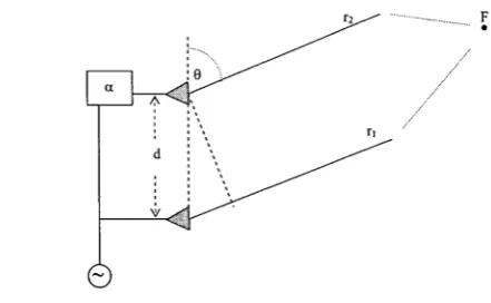
In order to get better insight into the beamforming technique, we present a simple example by calculating the radiation pattern for a two-antenna array. The aim is to calculate the strength of the electric held E at point F due to the radiation from the antennas as shown in Fig. 1.1. At point F, which belongs to the antenna far-held, the narrowband received held is given by

Ef = E0e~ir' + E0

__ Eoe~iri + cos 9 + a )

— EQe~iri( 1 + e *(fcu,dcos0+a)j

where 7q, r 2, d, a, 9 are defined as in Fig. 1.1; Block denoted by a represents a multiplier etaj ku = 27r/A is the angular wavenumber.

Further the modulus of the electric held E received at point F can be calculated as

|£>| = |£ b |- |( l + e * )| 'ip = k^d cos 0 + a

1.2. MULTIPLE ANTENNAS 6

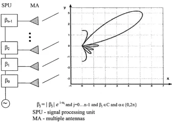
SPU MA

i a,

SPU - signal processing unit MA - multiple antennas

X

Figure 1.2: Beamforming technique with n-antenna array

while |(1 + e1^)I is the array factor. Similarly, the calculation can be repeated for the general case of phase beamforming, i.e., the antenna array with n antennas shown in Fig. 1.2. Then, the antenna array radiation pattern is given by

I

In the beamforming arrangement, once the signals are combined, the whole array has a single antenna pattern as graphically presented in Fig. 1.2.

1.2. MULTIPLE ANTENNAS 7

Receiver

Detector

Adaptation

Co-phasing and summation

Figure 1.3: Diversity combining technique

Beamforming techniques can be broadly divided into two categories: con­ ventional (fixed) beamformers and adaptive beamformers. In the conven­ tional beamforming technique, a fixed set of weightings \ßß and phase shifts eiaj is used to combine the signals from the antennas in the multiple antenna system. Based on the information about the locations of the antennas in space and the wave directions of interests, the fixed weights ßj are calculated in the signal processing unit (SPU). In the case of adaptive beamforming techniques, the weights are automatically updated by using the information about the antenna locations and wave directions, as well as the information extracted from the received signals. As the name indicates, in an adaptive beamforming technique, the response is automatically adapted and updated to different channel conditions and received signals variations.

1.2. MULTIPLE ANTENNAS 8

downconversion

downconversion

downconversion

space-time processing and decoding upconversion

upconversion upconversion space-time

layering and coding

Figure 1.4: Spatial multiplexing technique

Selection diversity is the simplest of these methods. From a collection of n antennas the branch with the largest signal-to-noise ratio (SNR) at any time is selected and connected to the receiver. As one would expect, the larger the value of n the higher the probability of having a larger SNR at the output.

Maximal SNR ratio combining takes a better advantage of all the diver­ sity branches in the system, and its block scheme is presented in Fig. 1.3. All n branches are weighted with their respective instantaneous signal-to-noise ratios. The branches are then co-phased prior to summing in order to en­ sure that all branches are added in phase for maximum diversity gain. The summed signals are then used as the received signal. The maximal SNR ra­ tio combiner has advantages over selection diversity but is more complicated. Proper care has to be taken in order to ensure that signals are cophased cor­ rectly and gain coefficients are constantly updated.

A variation of maximal ratio combining is equal gain combining. An equal gain combiner adjusts the phases of the desired signals and combines them in-phase after equal weighting. The output is a cophased sum of all the branches.

1.3. CLOSELY SPACED MULTIPLE ANTENNAS 9

In this case, an appropriate signal processing technique at the receiver can separate the downstream signals. A basic condition is that the number of receive antenna elements is at least as large as the number of transmit anten­ nas. This technique allows the data rate to be increased by a factor equals to the minimum between the number of transmitting and receiving antennas. The spatial multiplexing technique will be further investigated later in this thesis.

1.3

C lo se ly S p a c e d M u ltip le A n te n n a s

1 .3 .1 M u tu a l C o u p lin g E ffect

When antennas are closely spaced to one other, some of the energy that is primary intended for one antenna ends up at the adjacent antennas. Thus, the received signal of each antenna reflects not only the magnitude of direct incoming electromagnetic waves, but also some portion of the signals induced by the adjacent antennas. The effect is known as mutual coupling.

The portion of signal that will be induced from the adjacent antennas depends on a number of parameters. We summarize the most important parameters affecting mutual coupling.

• Separation between antenna elements is the most crucial parameter affecting mutual coupling. Analytical studies [5] have shown that if the antenna spacing is equal to or greater than a half of a wavelength, mutual coupling is negligible. This implies that mutual coupling will also depend on the frequency of the signals being received since the distance is expressed in terms of the wavelength;

1.3. CLOSELY SPACED MULTIPLE ANTENNAS 10

array. Elements on the periphery of the antenna array are less affected by the reradiated signals than the other antenna elements;

• Radiation characteristics of antenna is one of the factors determining mutual coupling level among the multiple antennas. This can be il­ lustrated by the following example which considers the two antennas case. If both antennas are transmitting, some of the energy radiated from each will be received by other because of the nonideal directional characteristic of practical antennas. Part of the incident energy on one or both antennas may be rescattered in different directions allowing them to behave as secondary transmitters [4]. Similar analysis can be obtained for the receiving mode of antennas;

• Relative orientation of antennas in the multi-antenna array plays an important factor determining the level of mutual coupling. As an ex­ ample, mutual coupling could almost vanish if dipoles are orthogonally positioned to each other, as it has been shown in [10];

• Another parameter that affects mutual coupling is direction of arrival (DoA). Studies have shown that mutual coupling and DoA are strongly coupled [11]. This effect mostly occurs in adaptive antenna arrays. In order to direct the antenna beam to a specific angle, the phase shifters in feeding network need to be adjusted, resulting in a different feed­ ing network and hence different mutual coupling scenarios. Moreover, waves impinging on antennas from different angles generate surface waves in different directions, which results in different mutual coupling; • Surrounding objects in the near field of the antenna elements affect

mutual coupling. Re-radiated signals from antenna elements can be reflected back from the near-field scatterers and be coupled back to the other elements, resulting in more coupling.

1.3. CLOSELY SPACED MULTIPLE ANTENNAS 11

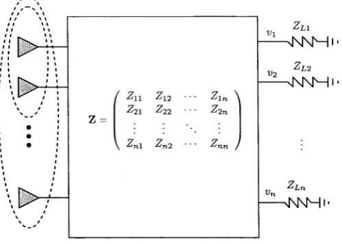
/ / "“ N \ / / \ \ / / > \

( Zn Z12 Z21 ^ 2 2 V ^ n l ^ n 2

^ln \ Z2n

Znn /

l’l ZlA

-sN S M i'

Zl2

-nN N Hi

\ t >

Z Ln -nN S Hi'

Figure 1.5: Network representation of multi-antenna system with coupled antennas

account because of its significant impact on system performance. There­ fore, we discuss network modeling and simulation methods that account for mutual coupling in the next section. We also outline the method used for simulation analysis in this thesis.

1 .3 .2 M o d e lin g o f C lo se ly S p a c e d M u ltip le A n te n n a s

The multi-antenna array can be regarded as a n port network with n ter­ minals (shown in Fig. 1.5). If the vector of induced currents is written as

i = [Zi, Z2, »An]T

where (.)T denotes transpose, and the vector of terminal voltages is given by

V = [ui,u2, ...,vn]T

the circuit relation at the n-port network can be written as

v = ZTi (1.1)

1.3. CLOSELY SPACED MULTIPLE ANTENNAS 12

matrix is a diagonal matrix defined by Z = Z& In

where is antenna impedance and In is the identity matrix of order n. However, in the presence of mutual coupling, the matrix becomes full rank, known as the mutual impedance matrix, and is defined by

Z n • • • Z ln ^ Z22 • • • z2n

Zn 2 • • • Znn J

Here, Z3\ is antenna self-impedance for j = /, while Zji is the mutual im­ pedance for j ^ l.

In order to calculate the mutual and self impedances, one should employ mathematical techniques and tools of the electromagnetic (EM) analysis. The EM analysis is a complex task, and there is no need to describe it in details here. However, understanding of the basic methods used in the EM analysis is of crucial importance, as it enables the most appropriate choice of parameters for analysis and accurate interpretation of the obtained results. Therefore, we present three basic methods often used in the EM analysis. In the order of increasing accuracy and complexity these methods are:

• the induced electromotive force (EMF) • the method of moments

• the full-wave electromagnetic numerical computation

In each method, an n^-element antenna array is represented as an iV-port network. For induced EMF, N = tla, while for the method of moments,

N is an integer multiple of i.e., each antenna is subdivided into equal- length increments, each corresponding to a port. Full-wave electromagnetic numerical computation assumes that the entire antenna is represented by a three-dimensional (3-D) computer-aided design model, and subdivided into N surface patches.

The calculation of the driving point impedance of each port by using those three methods is presented in the following.

Z u

Z21

1.3. CLOSELY SPACED MULTIPLE ANTENNAS 13

Induced EMF

Induced EMF is a classical method of computing the self and mutual im­ pedances of a N—port network representation of an antenna array. Here, the Poynting vector, created from the electric and magnetic fields, is inte­ grated over the array elements. This method is restricted to straight and parallel elements in formation and does not account for radii of the wires and the gaps at the feeds. The advantage of induced EMF is that it leads to closed-form solutions providing a simple analysis. As an example, following the approach of King [12], the elements of the mutual impedance matrix Z, can be calculated as

30(0.5772 + ln(2k J ) - Ci(2k j ) ) + 30(Si(2k j ) ) , m = n

Rmn T Arnni Vfl 7^ Vi

(1.2)

Rmn = 30cos(2/cu;/)(Ci(rxo) + Ci(u0) — 2Ci(rzi) — 2Ci(ui) + 2Ci(kud)) + 30sin(2/cw/)(—Si(u0) + Si(u0) + 2Si(wi) — 2Si(vi))

+ 30(—2Ci(wi) - 2Ci(v!) + 4Ci(fcd))

X mn = 30 cos(2kul)(—Si(u0) — Si(u0) + 2Si(iti) + 2Si(ui) — 2Si (k^d)) + 30sin(2/cw/)(—Ci(wo) + Ci(u0) + 2Ci(wi) — 2Ci(ui)) + 30(2Si(ui) + 2Si(ui) - 4Si(kud))

u0 = ku ( V d2 + 4/2 - 2/)

ui = ku ( V d2 + l2 - l)

Vo — ku( V d2 + 4/2 + 21) vi = k ^ V d ^ + l 2 + l)

1.3. CLOSELY SPACED MULTIPLE ANTENNAS 14

dipole antenna, and ku = 2 n /\ is the wave number. Since the above ex­ pressions only depends on interelement distances, arbitrary arrangements of array elements can be considered.

M e t h o d o f M o m e n ts

For greater accuracy, we may partition each antenna of the array into equal- length segments and apply the method of moments. The method of moments is a general technique for converting a set of linear integrodifferential equa­ tions into an approximating set of simultaneous algebraic equations suitable for solving on a computer. Using electromagnetic theory and assuming uni­ directional current flow, the current and charge densities are approximated by viewing the antenna arrays as filaments of current and charge of the wire axis. Using the method in [13], an expression for the mutual impedance matrix elements 1 < m, n < N is shown to be

Z m n iiO[ l A l n • l rn 'ljj(^Tl^ T fl)

where g is the horizontal distance between the antennas containing points n and m, a is the dipole antenna radius, ku is the wave number, zm is the vertical distance between the points n and m, /i is the permeability, e is the permittivity, Aln the length of the nth increment, u is the frequency of operation (in radians per second), and n~ and n + denotes the starting and terminating points of the nth increment, respectively.

F u ll-w av e E l e c tr o m a g n e tic N u m e r ic a l C o m p u t a t i o n

Full-wave electromagnetic numerical computation models both the electric current on a metallic structure and the magnetic current representing the field distribution on a metallic aperture. An element of the mutual impedance

+ -— ['ip(n+, m +) — xb{n , m +) —'0(n+, m ) + ij)(n , m )]

1.4. SUMMARY OF APPROACH 15

matrix Z, is given as

m n {ZsB m ■ Bn}ds s

J s Js (1.3)

where Zs is the surface of the antenna increment with surface 5, B n( r ) is a basis function, and G(~r \ ~r') is Green’s function. The differences among full-wave electromagnetic numerical computation formulations are based on the choice of basis functions B n(S^) for the current distribution representa­ tion and Green’s functions G{/r\~r ).

S O N N E T ® software uses a sum of sines and cosines as Green’s func­ tion, while some other electromagnetic software such as Zetland IE3D, uses the Sommerfield integral as a Green’s function [14]. Although, it is hard to make a comparison between different techniques and tools for the EM analysis, for a simple antenna array structure such as uniform linear array with half-wave dipoles, sufficiently accurate results can be obtained by using any of previously mentioned software, S O N N E T® , Zeland IE3D, or other similar software. On the other hand, for complex antenna structures, mul­ tiple EM tools are required in order to efficiently solve Maxwell’s equations. In any case, the understanding of the used method is essential as it enables the most appropriate choice of parameters for calculation, and the correct interpretation of the simulation results.

1.4

S u m m a r y o f A p p r o a c h

In this chapter, we first summarized the theoretical and practical features of multiantenna elements for use in mobile wireless communication networks. Then, we indicated on the potential limitations caused by implementing multi-antenna systems with small antenna spacing.

1.5. STRUCTURE OF THIS THESIS 16

In order to investigate the signal and noise coupling, we elaborated on the mutual coupling effect in this chapter. We presented a model of mutual coupling effect in multi-antenna systems (used in this thesis). Then, we discussed the three basic methods often used for mutual impedance matrix calculation, including the full-wave electromagnetic numerical computation, that has been used in this thesis.

1.5

S t r u c t u r e o f th is T h e s is

In this thesis, we provide an analysis of the mutual coupling effect on thermal noise. Then, we estimate the channel capacity of multi-antenna systems with small inter-element spacings.

In order to provide a better insight into the thesis topics, and to improve the clarity of presentation of the research results, the thesis is divided into two parts. The first part is focused on the signal processing theory, more precisely, the signal and noise coupling in the multi-antenna systems. In the second part, the achievable information rate of a wireless communication link is estimated when a coupled multi-antenna system is used at one side, or on both sides of the link.

1.5.1 Q u e s tio n s t o b e A n s w e r e d in t h i s T h e s is

In this thesis the following open questions are addressed: 1. Part I

• Does mutual coupling affect thermal noise?

• What is the impact of mutual coupling on thermal noise power in closely spaced multiple antennas?

• What is the overall effect of mutual coupling on signal-to-noise ratio in multi-antenna systems?

• What is the critical antenna spacing beyond which the combined mutual coupling can be neglected?

1.5. STRUCTURE OF THIS THESIS 17

• How does correlated noise affect ergodic channel capacity of MIMO wireless systems?

• How does correlated noise impact outage channel capacity, and cumulative distribution function of channel capacity?

• What is the minimum antenna spacing beyond which the channel capacity is not affected by mutual coupling?

• How many effective degrees of freedom can be formed in MIMO wireless system with coupled antennas?

• Could we separately estimate the total contribution of the noise correlation on the channel capacity?

1 .5 .2 C o n te n t an d C o n tr ib u tio n s o f T h e s is

In the following, the chapters of the thesis are outlined with emphasis on contributions made within:

Part I

Chapter 1 is the introduction chapter into the first part of the thesis. The system with multiple antennas, its advantages and typical applications, is elaborated. The mutual coupling effect is considered in the multi­ antenna systems. The modeling of the coupled multiple antennas, and the calculation method of the elements of the mutual impedance matrix are also presented.

1.5. STRUCTURE OF THIS THESIS 18

Chapter 3 examines the combined effect of noise and signal coupling in the multi-antenna systems. We investigate the combined effect of mutual coupling on signal and noise on the signal-to-noise ratio performance. Our simulation results indicate that the signal-to-noise ratio in coupled multiple antennas is underestimated if the noise coupling effect is not accounted for.

Chapter 4 is the concluding chapter of the first part of the thesis.

Part II

Chapter 5 represents the introduction into a wireless communication the­ ory. We examine the MIMO channel models found in the literature. In particular, we elaborate on the channel model that has been found as the most suitable for our analysis. We present the correlation model which introduces the signal coupling into the MIMO channel model. Chapter 6 - the concept of noise coupling is introduced into the channel

capacity calculations of MIMO systems with small antenna spacings. Channel capacity performance of the MIMO systems is estimated by varying the antenna spacing which has the greatest influence on the coupling level in the multi-antenna systems. Ergodic channel capac­ ity is investigated by applying equal power allocation and water-filling power allocation schemes at the transmitters. Furthermore, capacity outage and its cumulative distribution function are presented for very small antenna spacing along with the case when antennas are separated for more than a half of wavelength. The number of effective degrees of freedom is then examined. Noise correlation factor is derived, en­ abling the quantification of the noise correlation contribution to the channel capacity. Finally, an upper bound of the channel capacity of the coupled multi-antenna systems is defined.

1.5. STRUCTURE OF THIS THESIS 19

conjugate matching network is optimal in terms of signal power, and it also acts as the whitening filter on the coupled thermal noise. Fur­ ther, the capacity of MIMO systems is estimated when the coupled multi-antenna systems is used at both sides of the link, receiver and transmitter. Our simulation results confirm that the transmit coupling degrades the capacity performance compared to the case with no con­ straint on the emitted power.

C h a p te r 2

C o rre la te d N oise

2.1

In tro d u c tio n

Mobile wireless communication system design comprises a comprehensive setup of tasks with the core objective to attain the minimum achievable received signal power level to enable reliable transmission over a wireless channel. In a noise limited environment, the minimum received signal power level Ps can be defined as

Ps [dBm] = S N R min[dB] + Pn[dBm] (2.1) where S N R min is a minimum signal-to-noise ratio and Pn is a noise power level.

Therefore, the transmission quality criterion for the wireless system design can be defined as a minimum signal-to-noise ratio (SNR) at the receiver to achieve a pre-defined threshold for reliable communications. For digital systems, the transmission quality is defined in terms of the bit error rate (BER) and is driven by a range of factors such as modulation schemes, coding, etc. However, the SNR still persists as an essential parameter in determining the transmission quality of digital systems.

In a multi-user setting, an additional limitation is placed on the design of wireless systems where the interference from other users can significantly reduce the capacity performance of wireless systems. The presence of strong interferences is generally equated to a very noisy environment when the

2.2. ANTENNA NOISE 21

terference attains the AWGN characteristic, and it has been an established belief, prior to 1988 [15], that correct detection and demodulation is impossi­ ble. However, it was demonstrated in [15,16] and other papers that by using multiuser detection it is possible to combat multiuser interference in mobile wireless communication systems. Multiuser detection is based on the idea of detecting interference, and exploiting the resulting knowledge to mitigate its effect on the desired signal. Using such techniques, interference becomes less detrimental then noise [17].

From the previous discussions, one can conclude that the noise becomes a crucial factor in determining the transmission quality over the wireless channels even for multi-user mobile communications. In this context, we provide an analysis of the received noise in a multi-antenna system, while we examined the effects of signal-to-noise ratio at the receiver in Chapter 3.

In the next section, antenna noise is elaborated. This is followed by an interpretation of the noise coupling effect in the multi-antenna systems in Section 2.3. An analytical evaluation of the correlated noise in the multi­ antenna system is given in Section 2.4, while, simulation results are pre­ sented in Section 2.6. Concluding remarks and contributions are listed in Section 2.7.

2.2

A n te n n a N o ise

The noise appearing at the output of a receiver has its origin partially in the receiver and partially outside the receiver. The external noise is picked up by the antenna and is generally referred to as “antenna noise” . This type of noise is largely either man-made or environmental in origin.

2.2. ANTENNA NOISE 22

In summary, the dominant antenna noise for mobile wireless applications is thermal noise. However, impulse noise may be a predominant disturbance for some indoor situations. Therefore, both the thermal and impulse noise will be elaborated in the following.

2.2.1

T h e rm a l N oise

Noise is the result of the random motion of charged particles in a conductor. In general, the mechanical motions of these charged particles are coupled with other forms of energy such as the incident radiation energy on an antenna. When the charged particles are in thermal equilibrium with all other forms of energy with which they might be coupled, the noise is called thermal noise.

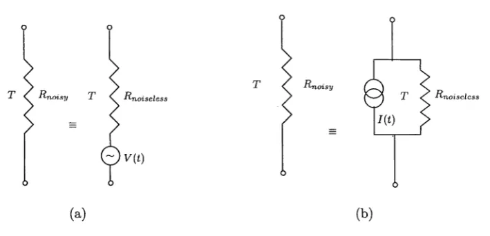
Because of the continuous thermal agitations of the charged particles, a random current I(t) exists. If a sufficiently sensitive ammeter is placed across the conductor’s terminal, a fluctuating reading would be observed. In similar way, a voltmeter would show a fluctuating voltage V{t). Schematically, this conductor can be represented as a noiseless resistance in series with a voltage source, with a spectral intensity proportional to that of the current generated therein as depicted in Fig. 2.1(a). Similarly, the conductor as a current source in parallel with a noiseless resistance can be presented as shown in Fig. 2.1(b).

The noiseless resistance in either instance has the same numerical measure as the actual, noisy one. Since V(t) = I ( t ) R, the spectral intensities are (in steady or equilibrium state) related by

W v (f) = R 2W, ( f ) (2.2)

where Wj(t) and Wy{t) are current and voltage spectral densities, respec­ tively. They were derived in two ways:

1. Directly on the basis of a kinetic-theory model of conduction process. Originally, it was presented in [19-21];

2.2. ANTENNA NOISE 23

o ₉

o o

T

T

b

6

(a) (b)

Figure 2.1: Equivalent representations of a resistance (at temperature T): (a) resistance represented as a noiseless resistance in series with a voltage source (b) resistance represented as a current source in parallel with a noiseless resistance

The former has the advantage of explicitness. The later is more abstract, while avoiding some of the technical difficulties inherent in any detailed model of the conduction process. Then, the voltage spectrum becomes

where k = 1.3806503 x 10~23J / K is the Boltzmann constant, and T is the absolute temperature in K.

The result (2.3) is strictly speaking, valid only for the low-frequency end of the spectrum. If this relation were used for all frequencies, the power spec­ trum W y ( f ) / R = 4 kT would then be independent of frequency in this model and one would have an infinite total power. In his original paper [22], Nyquist indicates that the difficulty can be overcome by replacing the equipartition value kT for the energy per mode of one-dimensional transmission line by Planck’s expression, as follows

hf (ehf/kT - l ) ' 1

where h = 6.6260692 x 10~34J s is Planck’s constant, and / is frequency. Then, the voltage spectral density becomes

2.3. NOISE COUPLING 24

wvV)

^7wrr~i

^

Thus, the spectrum departs noticeably from its constant low-frequency value at about / = (k / h ) T = 2.1 x 10loT Hz.

Now, the mean power P dissipated in the resistive element can be calcu­ lated as

P = W , ( f ) R ( f ) d f = 4KT R ( f ) 2\Y(iui)\2df

Jo Jo

roo

= / Wv (f)\Y(iu)\2df

(2.5)

(2.6)

where Y (iw) is admittance, and co is angular frequency. Here, the finite power is due to the frequency selective properties of the circuit, and not to the actual high-frequency behavior of the resistive element, since the “low- frequency” approximation is assumed.

Additionally, the general Nyquist’s formula for voltage and current spec­ tral density is valid for a general (linear passive) network when different resistances in the network are no longer at the same temperature. Then the spectral distribution of the total mean squared current fluctuations is the

sum of the current spectral densities of each resistance [23]

W ,U ) = (2.7)

t 1

where Zei is an equivalent resistance of the source Ei [24]. This result is experimentally confirmed in [25].

2.3

N o ise C o u p lin g

In this Section, we investigate the electromagnetic coupling of the thermal radiation intercepted by antenna elements.

2.3. NOISE COUPLING 25

2 .3 .1 T h e r m a l N o is e E l e c t r o m a g n e t i c R a d i a t i o n

Thermal noise electromagnetic radiation results in self-induced noise, also known as self-radiated thermal noise of an antenna element [26]. Further­ more, when an antenna element is placed in the close proximity of other radiated bodies, including the adjacent antenna elements, thermal noise is induced from the closely spaced radiated bodies [26]. It was predicted by [27] that the partially correlated noise is induced into two closely spaced antennas with isolated receivers. Theoretical formulation of this effect is given by the Nyquist thermal noise theorem [28].

2 .3 .2 N y q u is t T h e r m a l N o is e T h e o r e m

The generalized Nyquist thermal noise theorem [28] allows us to determine thermal noise power of coupled antennas in a multi-antenna system. The theorem states that for a passive network in thermal equilibrium it is possi­ ble to represent the complete thermal-noise behavior by applying Nyquist’s theorem independently to each element of the network.

In general, a network (even nonreciprocal) with a system of na internal thermal generators all at absolute temperature T is equivalent to the source- free network together with a system of noise voltage generators Em,m = l,...,n ^ with zero internal impedance [27]. Noise generator voltages are correlated and spectral density of their cross-correlation is given by (relates to the two coupled antenna case in Fig. 2.2(a))

where (•) denotes expectation, Zmn and Znm are the mutual impedances, and k is Boltzmann’s constant and T is absolute temperature. Similarly, spectral density of the nodal current cross-correlation is

(2.8)

= 2 kT + (2.9)

2.3. NOISE COUPLING 26

— h

Zl, Z L2

(a)

(b)

Figure 2.2: (a) Two coupled antennas and corresponding representa­

tion of their self ( Z n , Z 22), mutual ( Z i2, Z 21) and load im­

pedances (b) Network representation for two antenna array with voltage noise

2.4. NOISE IN MULTI-ANTENNA SYSTEMS 27

system can be written as

Wee] =2/cT(Z + Z*) (2.10)

where (•)* denotes conjugate transpose or Hermitian transpose. Further, matrix of current’s spectral densities is

VFjjt = 2 k T (Y + Y*) (2.11)

where Z and Y are the mutual impedance and admittance matrices, respec­ tively; e and j are voltage and current vectors, respectively.

From (2.11) and (2.10), one can conclude that the cross-correlations be­ tween the voltages/currents of open thermal noise sources are directly pro­ portional to the real part of their mutual impedances and admittances. Based upon these properties, total exchangeable thermal noise power between the multi-antenna systems and load network will be calculated.

2.4

N o ise in M u lt i - a n t e n n a S y s te m s

Based on the Nyquist Thermal Noise theorem, the noise correlation matrix for the closely spaced antenna can be derived. The correlated noise current and associated noise power for the simplest case, the two-dipole array, are calculated [29]. Then, for the generalized case, the noise covariance matrix and correlated noise power for the multi-antenna system with n antennas, is presented [30].

2 .4 .1 T w o -a n te n n a C a se

One can write the noise voltage spectral densities as in Fig. 2.2(b) for the two-antenna array in terms of its current spectral densities W jk and spectral densities of noise voltage generators WEk by

WVl = Z n W j, + Z121TJ2 - WEli + WEl - ZL1W j, (2.12)

WV2 = Z21WJx + Z22WJx = WEl2 + W E2 - Z L2Wj2 (2.13)

2.4. NOISE IN MULTI-ANTENNA SYSTEMS 28

terms W Ehl , I = 1,2 are the voltage spectral density of the noise generator

associated with the load impedance of receiver Z u , l = 1,2 and l = 1,2

are the voltage spectral density of the noise generator associated with the

input impedance of the Ith antenna element, respectively.

Furthermore, the spectral density of noise currents can be expressed as

Wj, = i ^ r ( ( Z 22 + Z L2)(WBli + WEl) - Z21(WEl, + WEl))

Wj2 = - ± - ( ( Z „ + Zl1)(WeL2 + WE2) - Z12(WEli + WEl)) (2.14) where |Z A| = d e t(Z A) is determinant of the receiver front-end impedance

m atrix Za given by

Z A = Z \ \ + Z u

Z 2 1

(2.15)

The power spectral density of thermal noise absorbed in the receiver load

of the first antenna - W m ( f ) is

W N1( f ) = 1- ( Z h l + Z l 1) W J lj;(2.16)

Similarly, for the second antenna:

W N2( f ) = 1 ( Z L2 + (2.17)

Substituting the expressions (2.12) in (2.16) yields

WN1(f) = {2 \C \\Z \\ ( {Z22 + Z “ )(Z2*2 + Z^ We^ + We'.*})

— Z 2\ { Z 22 + ^ l 2)W ElE* — ^2 1 ( ^ 2 2 + Z L2)We*e2

+ Z 2 lZ'21(W EL2E.L2 + (2.18)

Using (2.8) for the cross-correlation of noise voltage spectral density, the

expression (2.18) becomes

w m { f ) = k T (-^t f j) ]- ((Z22+ Z L2)(Z'22+Z' L2)((ZLi + Z'L1) + (Z n +z;,))

— ^2 1 ( ^ 2 2 + Z l 2)(Zi2 + Z\2) — ^2i(^22 + ZL2){Zi2 + Z[ 2)

2.4. NOISE IN MULTI-ANTENNA SYSTEMS 29

The spectral density of total collected noise power in the received load of the first antenna consists of two parts:

1. its internal thermal noise from its own resistance; and

2. the externally received noise that is accumulated from space. Further, the external noise consists of two parts:

1. one that its own antenna amasses directly; and

2. the part that is indirectly gathered through adjacent closely-spaced antenna [31].

Similarly, the spectral density of thermal noise power of second antenna is

w N2(f) = k T ( ( Z n + Z M +Z-L1) ((ZL2+Z ’h2) + (Z22 + Z2*2))

- Z 12(Z'U + z [ 1) ( z 21 + - z ; 2(Zu + + z 2\)

+ Z12Z,*2((ZL1 + Z'L1) + + z * ,))) (2.20)

For a given receiver bandwidth B : the thermal noise powers accumulated in the receiver loads of the first and second antennas can be written as

Pni = / W N1( f ) d f J B

(2.21)

PN2=

f

J B

(2.22)

where (•) denotes the mean value.

2.4. NOISE IN MULTI-ANTENNA SYSTEMS 30

...

,,

• • ■ 2

„

„

M ulti-an len na System Loads

Figure 2.3: Block diagram of the receive subsystem including coupled an­

tenna array and loads

2 .4 .2 G e n e r a l C a s e

An equivalent linear network representation w ith internal noise sources of

the multi-antenna system with nR antennas is presented in Fig. 2.3. Based on block diagram in Fig. 2.3, the vector of the noise current j can be written as

j = (Z + Zl) - 1 • er (2.23) where is thermal noise voltage vector contributions from antenna’s and

load’s system impedances, Z is the mutual impedance matrix, and is load

impedance matrix.

Then, the cross-covariance m atrix of thermal noise current spectral den­

sities is given by

Wj(/) = (Z + ZL) - 1W jT( /) ( ( Z + (2.24)

By applying the Nyquist thermal noise theorem (2.10) for the network in

Fig. 2.3, the m atrix of the voltage cross-spectral densities is the contribution

from the thermal noise from antennas and termination impedances, and can

be calculated as

2.5. NOISE CORRELATION MATRIX - DEFINITION 31

Then, the m atrix of the spectral densities of the nodal noise currents can be

rewritten as

W j = 2kT(Z + Zl) - 1 ((Z + Z L) + (Z + Z L)*)((Z + Z L) - y (2.26)

Further, the m atrix of the thermal noise cross-power spectral densities can

be written as

WPn = 2fcTdiag((9M ZL)(Z + Z L) " ' ((Z + Z L) + (Z + Z L)*)((Z + Z L) ' l ) t) (2.27)

where diag(-) is diagonal operator, and Dde(-) denotes real part of complex

value.

The total thermal noise power dissipated at loads Z L is

P N = 2kTBTv{<Hc(Zh)(Z + Z L) - 1((Z + Z L) + (Z + Z L)*)((Z + Zl) “ 1)1) (2.28)

where Tr(-) denotes the trace operator.

The solution in (2.27) is general, and is valid for any multi-antenna sys­

tems. When the antennas are widely spaced, the mutual impedances are

negligible, and the total thermal noise power becomes the sum of individual

antenna thermal noise powers, as one can see from (2.27).

Ptv — 4 TijikTB (2.29)

note that it is assumed that isolated antenna are matched to the loads im­

pedance Z = Z*L.

Based on this analysis, one can conclude that the noise current correlation

m atrix (2.24) directly reveals the noise correlation. On the other hand, the

correlated noise power m atrix is the diagonal m atrix composed of the coupled

antenna noise powers. Yet, each element of the correlated noise power matrix

consists of noise intercepted by its own antenna, and the noise dissipated due

to the mutual coupling from the adjacent antennas.

2.5

N o ise C o r r e la tio n M a tr i x - D e fin itio n

In order to provide an comparative analysis of the signal-to-noise ratio and