Information-Theoretic Limits on Broadband Multi-Antenna Systems in the Presence of Mutual Coupling.

(1)

Systems in the Presence of Mutual Coupling. (Under the direction of Dr. Brian L. Hughes.)

Multiple-input, multiple-output (MIMO) systems have received considerable atten-tion over the last decade due to their ability to provide high throughputs and mitigate multipath fading effects. While most of these benefits are obtained for ideal arrays with large separation between the antennas, practical devices are often constrained in physical dimensions. With smaller inter-element spacings, signal correlation and mutual coupling between the antennas start to degrade the system performance, thereby limiting the deployment of a large number of antennas. Various studies have proposed transceiver designs based on optimal matching networks to compensate for this loss. However, such networks are considered impractical due to their multiport structure and sensitivity to the RF bandwidth of the system.

(2)

(3)

by

Pawandeep Singh Taluja

A dissertation submitted to the Graduate Faculty of North Carolina State University

in partial fulfillment of the requirements for the Degree of

Doctor of Philosophy

Electrical Engineering

Raleigh, North Carolina

2011

APPROVED BY:

Dr. J. Keith Townsend Dr. Alexandra Duel-Hallen

Dr. Griff Bilbro Dr. Brian L. Hughes

(4)

DEDICATION

(5)

BIOGRAPHY

(6)

ACKNOWLEDGMENTS

First and foremost, I would like to thank my advisor Prof. Brian Hughes for his guid-ance and support throughout my PhD career. I have greatly benefited from his technical expertise and intuitive approach toward problem solving. His excellent art of communi-cating ideas, critical analysis and professional attitude have been instrumental in making this experience truly rewarding.

I would also like to thank my committee members Profs. J. Keith Townsend, Alexan-dra Duel-Hallen, Griff Bilbro and Steve Shannon for their valuable feedback and com-ments.

I would always cherish the company of my fellow group members Carlo Domizioli and Yuhan Dong for providing a stimulating research environment and years of camaraderie. I would also like to thank one of our undergraduate students, David Fioramonti for his contribution with NEC simulations.

(7)

LIST OF TABLES

Table 2.1 MIMO-OFDM system parameters . . . 39

Table 3.1 Optimal parasitic network: Circular array N = 4, L = 2, dmin =

(11)

LIST OF FIGURES

Figure 1.1 Configurations: (a) Antenna selection (AS), (b) Reduced

full-complexity (RFC), (c) Full-full-complexity (FC) . . . 7

Figure 2.1 Typical wireless signal propagation environment . . . 13

Figure 2.2 Two cluster model for a wireless channel . . . 15

Figure 2.3 Typical wireless power delay profile . . . 17

Figure 2.4 sinc() pulse shapes for OFDM modulation . . . 19

Figure 2.5 Cyclic prefix in OFDM . . . 20

Figure 2.6 OFDM implementation . . . 22

Figure 2.7 MIMO channel model . . . 24

Figure 2.8 Water-pouring schematic . . . 31

Figure 2.9 Frequency selective MIMO channel, N = 2, d= 0.25λ, Nt= 15 . 40 Figure 2.10 Performance of receive diversity in i.i.d. MIMO channels . . . 41

Figure 2.11 Performance of receive diversity in correlated MIMO channels . . 42

Figure 2.12 Performance of antenna selection in i.i.d. MIMO channels . . . . 43

Figure 2.13 Performance of antenna selection in correlated MIMO channels . 44 Figure 3.1 A circuit model of a receiver with antenna selection and mutual coupling . . . 47

Figure 3.2 Circuit model of the antenna array and switching network . . . . 49

Figure 3.3 A circuit model of a circular array receiver with antenna selection and mutual coupling . . . 60

Figure 3.4 Configurations: (a) Uniform linear array (ULA), (b) Uniform cir-cular array (UCA) . . . 62

Figure 3.5 Traditional antenna selection (ULA): (5,2) . . . 65

Figure 3.6 Parasitic antenna selection (UCA): (4,2) . . . 67

Figure 3.7 Parasitic switching (ULA) . . . 69

Figure 3.8 Parasitic switching (UCA) . . . 70

Figure 3.9 Parasitic switching w/o antenna selection (ULA) . . . 72

Figure 3.10 Bandwidth sensitivity of optimal matching ([31]) . . . 74

Figure 4.1 A simple matching network . . . 78

Figure 4.2 Matching network and Darlington’s equivalent forZL . . . 80

Figure 4.3 Equivalent representation of Fig. 4.2 . . . 81

Figure 4.4 LOS communication illustration: System model . . . 83

(12)

Figure 4.6 Percentage loss in capacity for arbitrary bandwidths relative to

the optimal bandwidth . . . 89

Figure 5.1 Input and output wave vectors for a two-port network . . . 92

Figure 5.2 S-matrix representation of RF front-end . . . 96

Figure 5.3 Impedance matrix representation of a 2-element array . . . 100

Figure 5.4 Optimal matching implementation using decoupling networks . . 104

Figure 5.5 N = 2, d= 0.25λc . . . 111

Figure 5.6 Eigen-impedance VSWR and eigen-modes N = 2 . . . 113

Figure 5.7 Box-car matchingN = 2 . . . 116

Figure 5.8 Eigen-modes, antenna-Q fit . . . 119

Figure 6.1 Network model for MIMO-OFDM with mutual coupling (sub-carrier index suppressed) . . . 122

Figure 6.2 MIMO-OFDM channel, N = 2, d= 0.25λc, Nt= 15 . . . 135

Figure 6.3 Optimal solution . . . 136

Figure 6.4 Diversity-OFDM: Outage capacity vs. spacing,N = 2 . . . 137

Figure 6.5 Diversity-OFDM: Outage capacity vs. spacing,N = 4 . . . 138

(13)

Chapter 1 Introduction

During the last decade, multiple-input multiple-output (MIMO) systems have received tremendous attention from the research community and industry alike. This interest in MIMO wireless communications was sparked by the pioneering work of Foschini and Gans [39], [38], and Telatar [90], who showed that the use of multiple antennas at the transmitter and receiver combined with sophisticated signal processing can provide high spectral efficiencies in wireless channels with rich scattering environments. This has also led to commercial deployment and adoption of multi-antenna systems in many current and future cellular standards (UMTS, LTE), wireless local area networks (e.g., WLAN-802.11n), and wireless metropolitan area networks (WMAN-802.16e/WiMAX).

(14)

assumed a rich scattering environment such that the fading was spatially uncorrelated. Later, MIMO channel models that incorporate physical scattering and limited angle-of-arrival (AoA) and angle-of-departure (AoD) spread, were also considered [58], [84]. A study of the impact of spatially correlated fading on MIMO channel capacity can be found in numerous papers [19], [91], [23], [24].

Spatial multiplexing schemes, such as Bell-Labs Layered Space-Time Architecture (BLAST) [110], offer tremendous data rates by transmitting independent streams of data from multiple transmit antennas simultaneously and rely on advanced signal processing capabilities to separate them in space and time at the receiver. Prior to decoding, the MIMO channel is often estimated to aid equalization. A technique to estimate MIMO channels for Vertical-BLAST (V-BLAST) systems by use of training sequences was pro-posed in [65].

Space-time and space-frequency coding techniques that exploit the spatio-temporal and spatio-spectral diversity of a MIMO wireless channel have been shown to alleviate the problem of signal fading. For example, Alamouti’s block coding [2] is a simple yet powerful rate-1 code that transmits modulated symbols over channels with 2 transmit antennas to capture the diversity in space and time/frequency. The use of MIMO systems forfrequency selectivechannels has also been a focus of study, particularly in conjunction with spread-spectrum and multi-carrier modulation techniques, such as code-division multiple access (CDMA) and orthogonal frequency-division multiplexing (OFDM) [62], [73], [7]. MIMO-OFDM now forms the air interface of many existing and new standards, namely IEEE 802.11n and 3GPP LTE.

(15)

that the MIMO channel is appropriately decoupled by use of transmit precoding and receive decoding. Generalized linear precoder and decoder design for MIMO systems was proposed in [83]. The capacity of MIMO systems with CSIT can be found in [80], [44], [94]. The capacity of such systems is necessarily greater than or equal to those without CSIT. An analysis of diversity versus multiplexing capability of MIMO systems can be found in [122].

The benefits of deploying a large number of antennas at a transceiver come at the cost of an increased system and hardware complexity. Antenna selection (cf. [70], [54], [6], [47], [48]) is a scheme that tries to bridge this gap between complexity and the ben-efits offered by multi-antenna systems. Antenna selection systems are also popularly known as hybrid-selection/maximal-ratio-combining (H-S/MRC). Some of the work on H-S/MRC can be found in [103], [104], [105], [106], [107]. For spatially correlated en-vironments, several designs that improve the performance of selection diversity systems have been proposed, including spatial-FFT [71], phase-shifter based design [121] and RF pre-processing [67]. Some of the implementation issues in antenna selection have been discussed in [69].

1.1 MIMO and Mutual Coupling

(16)

mutual coupling).

Several studies have addressed the impact of fading correlation and mutual coupling on the performance of MIMO systems. For conciseness, we highlight here only a few that are relevant to our work. While the impact of correlated fading due to non-richness of the scattering environment has been a topic of interest for quite some time, studies addressing mutual coupling in MIMO systems involving detailed network analysis of the RF front-end have been a focus of research only recently.

An antenna is a transducer that converts EM signals into electrical signals which are processed by a radio-frequency (RF) chain, which consists of amplifiers, demodulator and analog-to-digital (A/D) converter. The EM wave incident on an antenna induces a voltage across the antenna terminals which is captured by the rest of the RF chain to be processed digitally. For antennas spaced a fraction of a wavelength apart, coupling presents a significant impairment. The current flowing in one element alters the voltage across the other. A key ingredient of modeling compact MIMO transceivers is analyzing the relationship between these terminal currents and voltages, while also incorporating the propagation characteristics and fading correlation into the system model. It is con-venient to model an antenna array as a multiport network with a Thevenin equivalent

antenna impedance matrix and an open-circuit voltage vector. In the absence of signif-icant coupling, such representations reduce to a bank of uncoupled two-port networks and the received signal is a trivial function of the voltage induced across the antenna terminals.

(17)

be eliminated. In practice however, antenna loads are fixed and special RF circuits called

matching networksare inserted between the antennas and the rest of the RF network in order to provide maximum power to the digitizer. Such an approach was considered in [99], [100] where the antennas were represented using thescattering-parameter matrix or

S-matrix. This study proposed optimal multiport matching networks, commonly referred to as conjugate matching, that decouple the antenna array and deliver maximum power to the rest of the network. By use of EM simulations, it was shown that the diversity gains of an array approach unity as the spacing between the elements is decreased. In this study, the receiver noise was assumed to be spatially-white.

The impact of receiver noise modeling on the system performance for compact transce-ivers has been considered by several authors. Gans evaluated the impact of antenna thermal noise [42] and (spatially-white) amplifier noise [43], separately. It was shown that matching networks offer no improvement in capacity when antenna noise is dominant, while they have significant impact for amplifier noise dominant scenarios. A more general noise model was presented recently in [29], [30] for state-of-the-art receivers, and an optimal matching network applicable to a variety of MIMO schemes was derived. It was shown that the performance is significantly altered by the location of noise in the RF chain and that mathematically, it was possible to completely eliminate coupling at all spacings and achieve performance close to an ideal system. However, this appears counter-intuitive because, as the antennas are brought close to each other, we expect the system to behave like a single-antenna system.

(18)

close as a quarter of a wavelength and preserve most of the capacity advantages of MIMO systems. However, conjugate matching networks are often considered impractical because of their multiport structure. They do however, provide an upper bound on the system performance - a useful benchmark to compare other transceiver design methodologies. In this dissertation, we consider relatively simpler architectures, such as antenna selection, and investigate alternate transceiver designs that seek to exploit coupling among the antennas.

Another issue with these optimal transceivers - the sensitivity of the diversity gains to the RF bandwidth of the system, was highlighted in [60], [31] recently. All studies thus far have addressed the problem of mutual coupling and optimal matching assuming a narrowband communication model. In this dissertation, we also investigate optimal transceiver designs of single- and multi-antenna systems for broadband communications in the presence of mutual coupling.

1.1.1 Antenna Selection

As noted earlier, the benefits of deploying a large number of antennas at a transceiver come at the cost of an increased system and hardware complexity. Typically, each antenna in a receive (or transmit) array is associated with a low-noise amplifier/LNA (power amplifier/PA), a demodulator (modulator) and an A/D (D/A) converter. Together these components constitute the RF chain, which can be expensive. In addition, employing more antennas requires sophisticated digital signal processing (DSP) and for small hand-held devices, it puts a burden on providing an extended battery life. All these factors pose a challenge to the wide scale deployment of multiple-antenna systems.

(19)

0.5λ

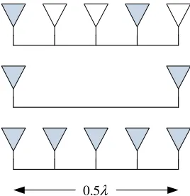
Figure 1.1: Configurations: (a) Antenna selection (AS), (b) Reduced full-complexity (RFC), (c) Full-complexity (FC)

and the benefits offered by multi-antenna systems. An antenna selection system with

N antennas and L RF chains, utilizes only L best of the available antennas (by use of a switching network) chosen based on the signal strength at each antenna. The signal from selected antennas is down-converted and fed to the digital signal processor. This reduces the number of RF chains required and hence the system and hardware complexity. Antenna selection systems is often compared with two of its popular counter-parts: (a)

full complexity (FC) and, (b) reduced full complexity (RFC) systems, with the same array size. Fig. 1.1 further illustrates these definitions. Unlike antenna selection, FC and RFC systems employ all of the available antennas, i.e., N and L, respectively. Under independent fading conditions, selection suffers a loss in performance compared to a full complexity system. However, the performance in the presence of mutual coupling is not well established.

(20)

rest of the array at all spacings. This assumption may not be valid for compact arrays. The other study [113], [114] models the inactive elements as terminated in the same impedance as the active elements. Although this may not seem like a problem when antennas are separated by large distances, we believe that terminating an inactive element in an impedance with non-zero resistive part will only absorb power and degrade the system performance. Besides, these studies have assumed a simplistic receiver model with spatially-white noise. As mentioned earlier, receiver noise modeling can play a crucial role in determining the system performance.

Traditional antenna selection schemes assume that the inactive elements are left open-circuited. While the termination of inactive elements does not matter when the array elements are uncoupled, it is imperative to study the role played by the inactive ele-ments in a compact selection system. One such study that explored this aspect was [120], wherein the impact of an open-circuited antenna placed close to a driven half-wavelength dipole antenna was studied numerically. The results show that, for small spacings and practical thickness of these dipoles, the open-circuited inactive elements can not be treated as transparent to the rest of the array.

(21)

open or short.

In this dissertation, we investigate ways in which coupling between the array elements can be exploited to improve the performance of selection systems. The key idea here is to use a different kind of termination that can reflect the power from the inactive elements in order to make more power available to the active antennas.

1.1.2 Coupling and Bandwidth

The other aspect of coupled multi-antenna systems that we study is the impact of mu-tual coupling on the RF bandwidth of the system, a relatively unexplored territory. As pointed out earlier, some studies have made a passing reference to conjugate matching networks diminishing the RF bandwidth of the system at close spacings [60], [31]. Match-ing networks built for systems with relatively large bandwidths fall under the purview of

broadband matching theory. Although a large body of research has addressed the issue of broadband matching for 2-port and uncoupled multiport networks (e.g., ideal MIMO systems), relatively little is known about MIMO broadband matching with mutual cou-pling.

(22)

dependence, it is imperative to study the design of matching networks for broadband transceivers.

Broadband matching theory was introduced by Bode in 1945 [5], when he addressed the design of alumped, reciprocal reactive 2-port network to match an arbitrarypassive, lumped load to a resistive source. Fano [35] established fundamental gain-bandwidth

trade-offs on broadband matching of a resistive source to a frequency-dependent load using Darlington’s equivalent of a load [27]. Youla [118] introduced an alternative way to solve this problem by use of complex-normalized scattering matrices. Chien [21], [22] further extended this idea to include frequency-dependent sources. Later, Chen [101] extended broadband matching theory to multiport networks. However, unlike our problem, these multiport networks were assumed uncoupled. The text by Chen [16] is an excellent reference for broadband matching theory and implementation techniques. In this work, we investigate the optimal end-to-end design of a broadband MIMO system in the presence of mutual coupling from an information theoretic perspective, while addressing the bandwidth limitations arising from broadband matching theory.

1.2 Overview of Dissertation

(23)

(24)

Chapter 2 MIMO for Wireless Communications

In this chapter, we introduce the building blocks of MIMO systems and develop channel and system models for a variety of MIMO communication schemes. This chapter shall serve as a launching pad for the remainder of this dissertation when we develop more generalized system models of compact MIMO transceivers in the presence of mutual coupling.

(25)

Figure 2.1: Typical wireless signal propagation environment

2.1 SISO Channel Model

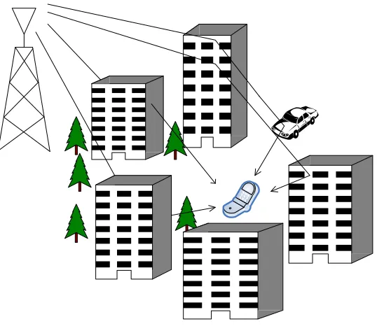
Fig. 2.1 shows a typical wireless signal propagation environment. The transmitted signal arrives at the receiver as a superposition of multiple delayed and attenuated copies -known asmultipaths, corrupted by additive white Gaussian noise (AWGN) at the receiver. If the complex baseband transmitted signal iss(t), the received signal can be represented by

r(t) = X

i

αi(t)e−j2πfcτi(t)s(t−τi(t)) +n(t) (2.1)

where, αi(t) and τi(t) represent the attenuation and propagation delay associated with

the i-th multipath at time t. Here, fc is the carrier frequency in Hz and n(t) represents

(26)

A wireless channel is typically characterized by two important time-domain parame-ters: delay spread and coherence time. Delay spread (Tm) is a measure of the maximum

delay between two (significant) multipath components

Tm = max

i,j,t |τi(t)−τj(t)| .

The reciprocal of delay spread is coherence bandwidth (Bc) defined approximately as

Bc ≈1/Tm. It is a measure of correlation in the frequency response of the channel. The

other channel parameter - coherence time (Tc), captures the time-varying nature of the

channel. It is a measure of how correlated in time, various multipath components are. It is usually measured as the reciprocal of Doppler spread (Ds) - maximum difference

between Doppler shiftsfcdτ_dti of each multipath

Ds =fcmax i,j,t

d

dt(τi(t)−τj(t))

.

Typically, the coherence time of a channel is much larger than its delay spread, i.e.,

Tm Tc. Such channels are sometimes called underspread channels.

Since the channel in (2.1) is linear, it can be described by a time-varying response

h(τ, t) =X

i

αi(t)e−j2πfcτi(t)δ(τ −τi(t))

(27)

1: ( 1, 1)

h α τ

2: ( 2, 2)

h α τ

Tx Rx

Figure 2.2: Two cluster model for a wireless channel

can model the channel as a linear time-invariant (LTI) system with an impulse response

h(τ) = X

i

αie−j2πfcτiδ(τ−τi) ,

such that

r(t) = Z

h(τ)s(t₋τ)dτ +n(t) .

For a system with passband bandwidthB (baseband bandwidthB/2), thesymbol du-ration(Ts) assuming Nyquist’s sampling theorem isTs = 1/B, such that the

continuous-time channel model can be written in discrete-continuous-time as a convolution with Nt-tap finite impulse response (FIR) filter 1

r[m] =

NXt−1

l=0

h[l]s[m₋l] +n[m] . (2.2)

A channel with B Bc, or equivalently Ts Tm is usually well modeled as a single-tap

1

(28)

filter (Nt = 1) such that the channel frequency response can be assumed to be fairly

constant over the entire bandwidth - hence the name frequency-flat channel. For an underspread, frequency flat channel, we can write

r[m] =hs[m] +n[m]

where

h ,X

i

αie−j2πfcτi

is called the fading path gain. It is modeled as the sum of a number of unresolvable

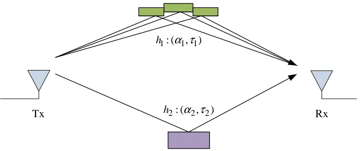
multipath components - multipaths with almost equal path delays [93], e.g., cluster 1 in Fig. 2.2.

Without any detailed knowledge of these individual multipaths within a cluster, h

is conveniently modeled as a random variable. Assuming a rich scattering environment

which has a large number of independent and identically distributed (i.i.d.) multipaths and no line-of-sight (LOS) component, (using Central Limit theorem) h is modeled as a complex Gaussian random variable with zero mean and variance σ2 ₌ P

iE[α2i]. The

amplitude |h| is thus Rayleigh distributed and phase φ = 2πfcτ is well modeled as

uniformly distributed over [0,2π). For this reason, such channels are also known as

Rayleigh fading channels.2 _{It is often the case that the channel remains constant over}

a number of symbols referred to as a block. For this reason, such channel models are also called block fading channels. The channel is assumed to vary from block to block and completely decorrelate in time with each block orrealization. When symbols are not

2

In the presence of a LOS component, the channel is usually modeled as havingRician fading

(29)

( )

Pτ

( s) τ µ

0 1 2 3 4 5

Figure 2.3: Typical wireless power delay profile

coded in time, it is convenient to assume a simplistic model

r =hs+n (2.3)

by dropping the time-index.

On the other hand, when B Bc multipath clusters are resolvable and the channel

is called frequency-selective. In such a case, the channel is can be modeled as an Nt-tap

discrete-time linear filter with coefficients hl at delays τl, l = 0, . . . , Nt−1. The fading

path gains are hl ∼ CN(0, σ2l). The strength of each multipath however, usually decays

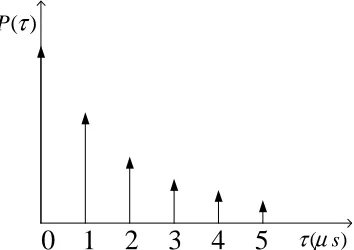
with time, since, the larger the delay, the greater thepath-lossthat the component suffers in propagation. The envelope of multipaths’ power vs. the delay is called the power delay profile(PDP) and is typically modeled as an exponential decay characteristic. It is a useful tool in analyzing a wireless channel’s temporal and spectral characteristics. An example PDP is illustrated in Fig. 2.3.

Based on the relationship between B andBc discussed above, frequency-flat channels

are also referred to asnarrowband channels and frequency-selective channels aswideband

(30)

fading and slow fading. This is usually associated with whether, for an application, one can transmit coded symbols over multiple fades of the channel (fast fading) or not (slow fading).

2.2 SISO-OFDM

In this section, we provide an overview of orthogonal frequency division multiplexing (OFDM) - amulti-carrier modulation technique suitable for broadband communications. For frequency selective channels, single-carrier transmission techniques such as code-division-multiple-access (CDMA) and wideband-CDMA currently deployed in IS-95 and UMTS systems, respectively, have been in use for cellular systems for quite some time now. However, OFDM is fast becoming the preferred choice in systems with large delay spreads owing to its ease of channel equalization.

(31)

Modulating Symbols

Figure 2.4: sinc() pulse shapes for OFDM modulation

OFDM makes it a suitable choice for transmission over channels that exhibit large delay spreads, (Ts Tm), or equivalently B Bc such that the channel is essentially

broadband. As the name suggests, in OFDM, information symbols are modulated over different frequencies referred to as orthogonal sub-carriers. Orthogonality is maintained by use sinc pulse shapes in frequency domain and modulating each sub-carrier at the center, as shown in Fig. 2.4. Given a passband bandwidth B, the number of sub-carriers

K is carefully chosen such that the sub-carrier spacing (∆f) is small compared to the coherence bandwidth of the channel

∆f = B

K Bc .

This ensures that each sub-carrier fades independently of each other and that the fading can be considered frequency-flat within each band.

(32)

Cyclic Prefix Tail

Original length- sequenceK

OFDM Symbol

Figure 2.5: Cyclic prefix in OFDM

pressed as

s[m] = √1

K

K_X−1

k=0

e

s[k]ej2πkm/K, m= 0, . . . , K −1

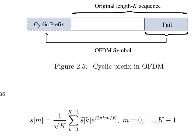
where _es[k] is the modulating symbol for the k-th sub-carrier. The time-domain OFDM signal utilizes a special structure which turns a frequency-selective channels into a set of parallel frequency-flat channels. The tail of s[m] comprising Ncp symbols, are copied as

is and appended to the beginning of the sequence - known ascyclic prefix (CP) or guard interval (GI) as shown in Fig. 2.5. The resulting sequence bs[m] is given by

b

s[m] =h s[K+Ncp−2] . . . s[K−2]s[K−1]

| {z }

cyclic prefix

s[0]s[1] . . . s[K₋1] i

The frequency selective channel can be represented by an Nt-tap discrete-time filter

h[m], m = 0, . . . , Nt −1, such that the channel output is given by the discrete-time

convolution

r[m] = h[m]∗bs[m] +n[m]

=

NXt−1

l=0

(33)

The length of CP ensures zero inter-symbol-interference (ISI) between consecutive OFDM symbols and also renders the otherwise linear convolution with the channel, circulant

r[m] =h[m]~_s_[_m_{] +}_n_[_m_]

From the property of circular convolution, we know that the DFT of the system is a point-by-point multiplication, i.e.,

e

r[k] =

K_X−1

m=0

r[m]e−j2πmk/K

= eh[k]_es[k] +_en[k] ,

where the accent tilde denotes a variable’s frequency-domain attributes.3 _{Henceforth, we}

shall use a subscript to denotek-th sub-carrier in place of [k]

e

rk=ehkesk+nek . (2.4)

For this reason, OFDM is known to turn a frequency-selective fading channel into a set of orthogonal frequency-flat fading channels. This provides tremendous savings in equalization at the receiver which is carried out in the frequency-domain4 _{with the help}

of channel estimation techniques using pilot sub-carriers - similar to training sequence in a time-domain channel estimation. In the absence of noise and perfect knowledge of channel gains for the k-th sub-carrier, the equation above emphasizes the frequency-domain equalization technique that is one of the biggest advantages of OFDM. The

3

Ifxdenotes a quantity in time-domain, we shall represent it in frequency-domain by the notationx_e

in the remainder of this dissertation.

4

(34)

QAM Mapper Serial to Parallel Converter Add CP & P/S Converter IFFT D/A

[ −1]

s K

cos(2πf t_c )

[ 1]

S K−

[1]

S

[0]

S s[0]

[1] s Detect Parallel to Serial Converter Remove CP & S/P Converter FFT and Equalization A/D [ 1]

r K−

cos(2πf t_c )

[ 1]

R K−

[1]

R

[0]

R r[0]

[1]

r

Figure 2.6: OFDM implementation

transmitted symbols are estimated simply as

e

sk = e

rk

e

hk

The frequency-domain channel for each sub-carrier is related to the channel impulse response by DFT

e

h[k] =

K

X

m=1

h[m]e−j2πkm/M , k= 0, . . . , K−1

where

h[m] =     

h[m] , 0< m < Nt−1

0 , m _≥L

     .

(35)

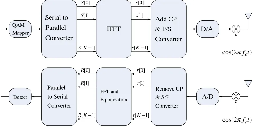
convenient to choose the number of sub-carriers to be a power of 2. Fig. 2.6 shows the basic modulation and demodulation techniques used in OFDM.

As can be seen, the overhead due to cyclic prefix in the OFDM symbol results in a loss in capacity but the trade-off over system complexity more than compensates for it. The OFDM symbol, thus spans a duration ofKTs+Tcp whereTcp=NcpTs is the duration of

cyclic prefix chosen such thatTcp > Td for zero ISI. At the receiver, the firstNcp samples

are discarded because of ISI from the previous OFDM symbol while the remaining K

symbols are directly equalized using the channel estimates for each sub-carrier. For more details about OFDM, the reader is referred to [79].

It is worthwhile to point out another advantage of OFDM (or for that matter, multi-carrier modulation) over single-multi-carrier techniques. It is the ability to adapt the power and bit loading using adaptive modulation on each sub-carrier independently. In other words, it provides the ability to achieve a discrete approximation of spectralwater-pouring

strategies. As we shall see later, some of the optimal power allocation schemes we derive shall exhibit a water-pouring characteristic.

2.3 MIMO Channel Model

Next, we consider a channel model for MIMO systems. To begin with, we consider only frequency-flat fading channels, i.e, single tap channels (Nt = 1); more generalized

frequency-selective MIMO channels will be dealt toward the end of this chapter. Consider a MIMO system withM transmit antennas andN receive antennas as shown in Fig. 2.7. Let s = [s1, s2, . . . , sM]T ∈ CM represent the complex-baseband transmitted symbol

(36)

1

M s

s

1

N r

r +

+

1

N n

n

11

NM h

h

1

N

M h

h

Figure 2.7: MIMO channel model

anN _×M channel matrixH and a receiver noise vector n= [n1, n2, . . . , nN]T ∈ CN by

r=Hs+n , (2.5)

a matrix version of (2.3). The noise vector at the receiver is assumed to be zero-mean, circularly-symmetric, jointly complex-Gaussian (ZMCSCG) in distribution, henceforth denoted as n _{∼ CN}(0,Rn) where, Rn = E[nnH] is the noise covariance. For now, we

assume that the noise covariance in general is non-diagonal. We shall elaborate on its structure and computation when we address the detailed receiver model used to represent transceivers with mutual coupling. The total transmit power is given by P0 = Tr(Rs)

where Rs=E[ssH] is thetransmit signal covariance.5

5

Throughout this dissertation, (_·)∗_{, (}_·₎T_{, (}

·)H_{, Tr(}

·) andE[_·] shall denote conjugation, transposition,

(37)

The elements of the MIMO channel matrix specified as

H=      

h11 . . . h1M

... ...

hN1 . . . hN M

     

are also ZMCSCG but are spatially correlated to an extent governed by the physical separation between the elements and scattering environment. In general, the correlation between any two entries of H is given by aN M ×N M block matrix

RH =

     

E[h1hH1 ] . . . E[h1hHM]

... . ..

E[hMhH1 ] . . . E[hMhHM]

    

 (2.6)

where hi denotes the i-th column of H. We denote this by H ∼ CN(0,RH).

Alterna-tively,RH =E[vec(H)vec(H)H], where vec(H) represents the vector obtained by stacking

the columns of H.

In MIMO literature, this correlation is often assumed to exhibit the separable cor-relation model behavior [58]. This is particularly true of scenarios when the transmit correlation from two transmit antennas is independent of the receive antenna from which it is observed (and vice-versa for receive correlation). In such a situation, the full corre-lation matrix can be written as a Kronecker product (denoted by⊗)

(38)

where, R_T = (1/M)_E[HH_{H] and} _R

R = (1/N)E[HHH] are positive-definite Hermitian transmitandreceive spatial-correlationmatrices, respectively. For this reason, this model is also known as Kronecker correlation model. The MIMO channel matrix can thus be simplified into a product of known spatial correlation matrices and an N _×M white

stochastic channel matrix Hw

H=R1/2_R HwR1/2T ,

where Hw ∼ CN(0,I) and Iis the N ×N identity matrix. Alternate models for MIMO

channels have been proposed in [84].

The extent to which the signals incident on two antennas are correlated is not only a function of the separation between them but also how dense the scattering environment is. For example, a base-station in a cellular network is located at a greater height and has less scatterers/reflectors in the vicinity. A cell-phone on the other hand, is usually surrounded by many objects outdoors or indoors. For this reason, antenna separation required to ensure least signal correlation is lower in cell-phones or portable devices, typically a few wavelengths, while that at the base-station is tens of wavelengths. For simplicity, we shall throughout this study, assume that transmit antennas have a separation large enough so that the signals are perfectly uncorrelated, i.e.,RT =Isuch that

H=R1/2_R Hw .

For a uniform linear array (ULA) with spacing d, the correlation matrix is [25]

[RR]_nm=

Z 2π

0

Z π

0

gn(θ, φ)g∗m(θ, φ)ej2πd(n−m) sinθcosφ/λp(θ, φ) sinθdθdφ , (2.7)

(39)

mul-tipaths arriving from (θ, φ), λ is the wavelength. When multipaths are uniformly dis-tributed in the plane p(θ, φ) = 1

2πδ θ− π 2

and scattering is neglected so each dipole is omni-directional gn(π₂, φ) = 1, (2.7) reduces to Clarke’s [25] formula

[RR]nm =J0 2π_λd(m−n)

(2.8)

where J0 is the zeroth-order Bessel of first kind.

2.4 Multi-Antenna Communication Schemes

In this section, we briefly discuss some of the popular communication schemes that utilize multiple antennas at the transmitter and/or receiver. We also present some of the relevant metrics to measure the system performance for MIMO systems. Although we address narrowband systems here, an extension to broadband MIMO systems is provided in the next section. Throughout this dissertation, we shall assume that perfect estimates of the channel are available at the receiver at all times, also referred to as channel state information (CSI). [65] highlights the aspects and methods of MIMO channel estimation through training sequences.

(40)

derived the Shannon capacity of a MIMO system in AWGN channel [90]

Cawgn = max Tr(Rs)≤P0

log₂det

I+ 1

M N0

HRsHH

(2.9)

where det(_·) denotes the determinant. In cases where the noise is spatially correlated, we have

C = max

Tr(Rs)≤P0

log₂det

I+ 1

MR

−1

n HRsHH

(2.10)

For a fast fading channel, however, it is appropriate to talk about the capacity in a statistical mean orergodic sense, expressed as

Cerg = max Tr(Rs)≤P0E

log₂det

I+ 1

MR

−1

n HRsHH

. (2.11)

In the absence of channel state information (CSI) at the transmitter, the optimal trans-mission strategy for (2.11) is equal power allocation across the transmit antennas [90]

Rs= P0

MI

and the capacity achieving transmit vectors have complex normal distribution.

On the other hand, for slow fading channels, a more accurate metric isoutagecapacity. Outage analysis quantifies the level of capacity that is guaranteed with a certain level of reliability. It is the probability that the capacity falls below a certain threshold or goes into an outage

(41)

For example, 1% outage capacity means the information rate Cout,1% is gauranteed for

99% of the channel realizations.

2.4.1 Eigen-Mode Transmission

In certain scenarios, it is possible that complete CSI is available at the transmitter. This information could either be delivered to the transmitter by the receiver through feedback or estimated at the transmitter through reciprocity arguments when the channel on the forward link (or downlink) is same as the one on reverse link (or uplink). For example, time division duplexing (TDD) systems use the same set of frequency bands for communication in either link which makes it possible to relay the CSI to the transmitter as control information through feedback.

When perfect CSI is available at the transmitter, it is possible to decompose the MIMO channel intor= min(M, N) orthogonal spatial modes with the help of appropriate

transmit precoding and receive decoding. To observe that, consider the singular value decomposition (SVD) of the channel matrix

H=UΣVH

where, U _{∈ C}N×N and V _{∈ C}M×M are unitary matrices representing the left-hand and right-hand singular vectors of H, respectively and Σ is a rectangular matrix whose diagonal elements are non-negative real numbers and off-diagonal elements are zero. The diagonal elements σ1 ≥ σ2 ≥ . . . ≥ σr are the ordered singular values of H, where

r=min(M, N). The squared singular values are the eigen-values of HHH:

(42)

Incorporating the SVD into the system model (2.5), we get

r0 = Σs0+n0

where, r0 =UHr, s0 =VHs and n0 = UHn represent equivalent vectors after a unitary linear transformation that preserves the energy of signals since _ks0_k2 = _ks_k2 and the distribution of noise n0 _{∼ CN}(0,Rn). The last equation represents a set of parallel

non-interfering ororthogonal channels

r0_i =σis0i+n0i .

The Shannon capacity can be represented as

Cawgn = max

Tr(Rs)≤P0

log2det

I+ 1

M N0

UΣVHRsVΣUH

= _Pmax

iγi≤P0

r

X

i=1

log₂

1 + 1

M N0

λi(HHH)γi

whereγi =E[|s0i|2] represents the power allocated toi-th eigen-mode. The optimal power

allocation is given by a spatial water-pouring solution [26], [62], [23]

γi =

F ₋ M N0

λi(HHH)

+

where, [x]+ _{= max}_{_x,₀_} _and_F _{is the water-level governed by the total power constraint}

r

X

i=1

(43)

Used modes

Unused modes

F

0 2 1

MN

σ

0 2 2

MN

σ

0 2 3

MN

σ

1

γ γ2

γ

3

Figure 2.8: Water-pouring schematic

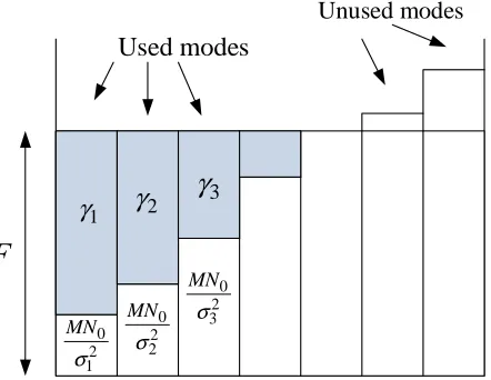
An illustration of this solution is depicted in Fig. 2.8. The optimal signal covariance can be computed using

Rs =V

     

γ1

. ..

γr

     

VH .

2.4.2 Spatial Multiplexing

(44)

error (MMSE), while successive interference cancellation (SIC) is a popular non-linear equalizer. The power allocation strategy (in the absence of CSIT) is uniform across space

Rs= P0

MI .

This idea was originally proposed by Paulraj and Kailath in 1993 and a working model was demonstrated at Bell Laboratories as V-BLAST [110].

2.4.3 Transmit and Receive Diversity

It is not necessary that a MIMO system be equipped with multiple antennas at both the ends of the communication link. A MIMO system with a single transmit antenna andN

receive antennas is referred to as aN-receive diversity system. AnM_×1 MIMO system is called a transmit diversity system. Here, we present a receive diversity system and a metric suitable for performance evaluation. The system model of a 1×N narrowband MIMO system can be written as

r=hs+n

where the lower-casehdenotes thechannel vector. With perfect estimates of the channel at the receiver, one of the most widely used linear combining technique is such that the input r to the combiner is linearly weighted w as

(45)

The optimal weight vector that maximizes the post-processing signal-to-noise ratio (SNR)

γ = |bh|

2

E[_|n_b_|2_] =E

|wHh_|2 wH_Σ_n_w .

is given by w = R−

1 2

n h where E = E[|s|2]. This technique is commonly referred to as noise-whiteningwithmatched filterormaximal-ratio-combining(MRC). Using Kronecker model, we can characterize the channel vector along with the receive spatial correlation

h=R1/2_R hw

where hw is the N ×1 i.i.d. fading path-gain vectorhw ∼ CN(0,I).

2.4.4 Antenna Selection

As outlined in Chapter 1, antenna selection offers a cost- and power-efficient way to realize the benefits of a multi-antenna system. In this section, we provide the system model for a simple receive antenna selection system and evaluate the performance for a variety of configurations toward the end of this chapter.

Consider a receiver with N receive antennas and LRF chains. The array is followed by a noiseless switching network that selects L out of N “active” antennas to connect to the L receiver RF chains. The remaining ¯L = N ₋L “inactive” antennas are left unattended. Let _S = _{s1, . . . , sL} denote the indices of the L active antennas, and

let ¯_S = _{s¯1, . . . ,s¯N−L} be the corresponding indices of the ¯Lc inactive antennas. The

received signal can be expressed as

(46)

where I_S is the _{|S| ×}N selection matrix defined by

[IS]ij =

    

1, if j =si

0, otherwise    

 , (2.12)

|S| = L is the cardinality of _S and hS = ISh. The receiver employs a linear combiner

similar to a diversity system. The optimal MRC is given by w= R−

1 2

n h_S such that the

optimal SNR for the antenna selection system is given by

γo = _Emax

IS k

R−

1 2

n h_Sk2 (2.13)

The optimal subset S is the one that maximizes 2.13. We assume a block fading channel such that the optimal subset is computed once every block.

2.5 MIMO-OFDM

In the previous sections, we discussed MIMO channel model for narrowband systems and the broadband transmission technique - OFDM, separately. In this section, we provide insights into MIMO channel models for frequency-selective channels and develop the system model for broadband MIMO communications in conjunction with MIMO-OFDM. Consider a MIMO-OFDM system6 _with _M _transmit, _N _{receive antennas and}_K

sub-carriers spanning a passband bandwidth B. First, we develop the wideband MIMO channel model by reusing some of the concepts developed in the SISO channel model section. Like wideband SISO channels, each entry of the MIMO channel matrix is essen-tially a multi-tap channel. Wideband MIMO channels can thus be modeled as a tensor

6

(47)

such that the channel impulse response’s l-th tap is given by a N _×M matrix

H_l =      

h11[l] . . . h1M[l]

... . ..

hN1[l] . . . hN M[l]

     

, l= 0, . . . , Nt−1

where the entries of Hl are ZMCSCG - Hl ∼ CN(0,RH). Here, we assume that the

time-invariant propagation environment is such that rich scattering near the transmitter and receiver ensures same transmit and receive spatial correlation for each multipath index [7]. The MIMO channel matrix for l-th multipath can thus, similarly be specified using the Kronecker model as

Hl =R1/2R HwlR1/2T .

Here, Hwl represents the stochastic N ×M white channel matrix having i.i.d. complex

Gaussian entries H_wl _{∼ CN}(0,I).

Like SISO channel models, the underlying complex baseband channel impulse re-sponse between r-th receive and t-th transmit antenna can easily be modeled by Nt

significant multipaths as

hrt(τ) = N_Xt−1

l=0

αrt[l]e−j2πfcτrt[l]δ(τ −τrt[l])

where αrt[l] is the attenuation and τrt[l] is the propagation delay associated with l-th

(48)

channels [76]. The frequency response of each MIMO link pair (r, t) at various sub-carriers is computed using a K-point FFT (K _≥L) of the MIMO channel impulse response as

ehrt[k] = K

X

n=1

hrt[n]e−j2πkn/M , k = 0, . . . , K −1

where

hrt[n] =

    

hrt[n] , 0< n < Nt−1

0 , n≥Nt

     .

The MIMO-OFDM channel matrix for the k-th sub-carrier is thus given by

e Hk =

     

e

h11[k] . . . eh1M[k]

... . ..

ehN1[k] . . . ehN M[k]

    

 , k= 0, . . . , K−1 (2.14)

An alternative representation of a MIMO-OFDM system with K sub-carriers, is an ex-tension of (2.4) such that the model is expressed in frequency-domain as

erk=Hekesk+enk , k = 1, . . . , K (2.15)

where, esk is the M × 1 transmitted symbol vector on the k-th sub-carrier, erk is the

N×1 received symbol vector andenk is theN×1 additive white Gaussian noise (AWGN)

vector at the receiver with zero mean and covariance R_en_k =E[ne_kneH_k], denoted by en_k ∼

CN(0,R_en_k). Observe that the equation above represents a set ofKorthogonal flat-fading

MIMO systems where the notation Hek emphasizes the frequency-domain nature of the

(49)

Owing to this orthogonal decomposition of the frequency selective channel, the cu-mulative MIMO-OFDM system can be represented in matrix notation by

r =Hs+n (2.16)

where, His a KN _×KM block diagonal matrix given by

H=       e H1 . .. e HK       (2.17)

and the corresponding vectors by

r =      

er1

... erK

      , s=      

es1

... esK

      , n=       e n1 ... e nK     

 . (2.18)

The Shannon capacity in bits/sec per Hz or spectral efficiency of the system is a simple extension of the narrowband MIMO Shannon capacity (cf. 2.10)

C = 1

K Tr(Rmaxs)≤KP₀

log2det

I+ 1

NR

−1

n HRsHH

(50)

where I is an N K_×N K identity matrix, Rs represents the transmit signal covariance

Rs = E[ssH]

=      

E[es₁_esH₁ ] . . . E[es₁_esH_K] ... . ..

E[esKesH1 ] . . . E[esKesHK]

      (2.20)

and Rn the noise covariance

Rn = E[nnH]

=      

E[en1neH1 ] . . . E[en1neHK]

... . ..

E[n_e_K_enH₁ ] . . . _E[n_e_K_enH_K]     

 . (2.21)

For spatially- and spectrally-uncorrelated noise with variance N0, Rn = N₀I. By em-ploying the SVD of the MIMO-OFDM channel matrixH, (2.19) can be decomposed into

r(H₎ _{space-frequency modes}_{such that the capacity can be rewritten as}

C = 1

K Pr(Hmax)

i=1 γi=KP0

  

r(_XH)

i=1

log₂

1 + γi

M N0

λi(HHH)

_

 .

Here,r(A) denotes the rank of matrixA. The optimal power allocation isspace-frequency water-pouring [80]

γi =

F − M N0

λi(HHH)

(51)

Table 2.1: MIMO-OFDM system parameters

Parameter Relation Value

Bandwidth (B) 20 MHz

Relative bandwidth (Br) B/fc 6.67%

Channel taps (Nt) 15

Power delay profile (Pd) exp(−nTs/Td)

Symbol rate (Ts) 1/B 50 ns

Max. delay spread (Tm) 0.8µs

Coherence bandwidth (Bc) 1/Tm 1.25 MHz

Max. Doppler (BD) 25 KHz

Coherence time (Tc) 1/BD (≈10TO) 40µs

OFDM symbol duration (TO) KTs+Ncp (≈5Tm) 4 µs

Sub-carriers (K) 64

Cyclic prefix length (Tcp) 16Ts 0.8µs

Carrier spacing (∆f) B/K 312.5 KHz

where F is governed by the total power constraint

r(_XH)

i=1

γi =KP0 .

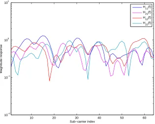
Example: Let us consider an example MIMO-OFDM system with M = 2 transmit antennas and N = 2 receive antennas. The OFDM system parameters are taken from IEEE 802.11a WLAN standard and listed in Table 2.1. Fig. 2.9 shows the frequency re-sponse for a 2_×2 MIMO system forK = 64 OFDM sub-carriers spread over a bandwidth

B = 20 MHz, with each MIMO link represented by Nt = 15 taps. The transmit

anten-nas are assumed to be spaced sufficiently far apart, while the spacing at the receiver is

d= 0.25λ. The spatial correlation matrix RRat the receiver is calculated using Clarke’s

(52)

10 20 30 40 50 60 10−2

10−1 100 101

Sub−carrier index

Magnitude response

H₁₁(f) H

21(f)

H₁₂(f) H₂₂(f)

Figure 2.9: Frequency selective MIMO channel, N = 2, d= 0.25λ, Nt= 15

address mutual coupling effects on the system model and derive information theoretic limits.

2.6 Performance in Correlated Rayleigh Fading

We conclude this chapter by presenting some results on diversity and antenna selection schemes discussed in previous sections.

2.6.1 Diversity

(53)

−5 0 5 10 15 20 10−3

10−2 10−1 100

Normalized received SNR (dB)

Probability

N=1 N=2 N=3 N=4 N=5

Figure 2.10: Performance of receive diversity in i.i.d. MIMO channels

of diversity systems with i.i.d. fading and noise with variance N0. The SNR E/N0

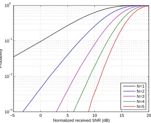
is selected to be 10 dB. Monte-Carlo simulations are carried out for 50,000 channel realizations. Fig. 2.10 shows the performance - on the x-axis, we have the received SNR and y-axis shows the probability that optimal SNR goes into an outage. For a given outage probability, the difference in received SNR compared to a single antenna system is described as thediversity gain of the system. Observe the huge diversity gains offered by diversity receivers as we increase the number of receive antennas. For example, at a 1% outage, N = 2 yields a gain of 14 dB while 19 for N = 3, 22 for N = 4 and 24 dB for N = 5. The gains however, become diminishing with each additional element.

(54)

−5 0 5 10 15 20 10−3

10−2 10−1 100

Probability

N=1 N=2 (corr) N=3 (corr) N=4 (corr) N=5 (corr) N=5 (iid)

Figure 2.11: Performance of receive diversity in correlated MIMO channels

illustrate the effects of correlation, we assume an exponential correlation model:

ρij =

    

e−β|i−j| _, _i₆₌_j

1 , i=j

    

whereβ >0. Fig. 2.11 shows the impact of fading correlation for the same set of systems considered above for i.i.d. scenarios. For high degree of correlation, the loss in SNR is noticeable, e.g., 5 dB and 3 dB withβ = 0.2 forN = 2 andN = 3, respectively.

2.6.2 Antenna Selection

(55)

−5 0 5 10 15 20 10−3

10−2 10−1 100

Probability

(5,1) (5,2) (5,5) N=1 N=2

Figure 2.12: Performance of antenna selection in i.i.d. MIMO channels

number of RF chains. The SNR _E/N0 is selected to be 10 dB. Fig. 2.12 shows the

(56)

−5 0 5 10 15 20 10−3

10−2 10−1 100

Probability

(5,1) (5,2) (5,5) N=1 N=2 N=5 (iid)

(57)

Chapter 3 Antenna Selection for Compact

Arrays

In the previous chapter, we have seen how receive diversity systems offer significant performance improvement over single antenna systems. However, we know that the use of multiple antennas comes at the cost of an increased overhead on hardware complexity and cost. Antenna selection on the other hand, offers a promising trade-off between cost and diversity benefits.

(58)

networks are considered impractical and expensive to build, leaving little but no choice than to space the antennas farther apart. In this chapter, we explore alternative avenues to construct low-cost multi-antenna transceivers with improved performance, using an-tenna selection.

As highlighted in Chapter 1, parasitic antenna structures can leverage significant per-formance improvement in compact arrays. By way of exploiting coupling, we investigate the design of a compact receive antenna selection system, that puts the inactive ele-ments at use. The underlying motivation is to come up with selection architectures that offer improved diversity performance, compared to a system without selection with an equal number of RF chains and array size. An illustration of this comparison is given in Fig. 1.1. It shows three systems with and without antenna selection, referred to as (a) antenna selection (AS), (b) reduced full-complexity (RFC), and (c) full-complexity (FC). We begin with a system model for antenna selection in the presence of mutual cou-pling. In Sec. 3.2, we formulate the problem for a selection diversity system and discuss optimal matching and optimal/sub-optimal parasitic network design. Sec. 3.3 outlines a numerical example and presents the results for various configurations. Sec. 3.4 pro-poses a simple yet powerful selection strategy that exploits coupling between the active and inactive elements. We conclude this chapter by summarizing the main findings and highlighting some implementation issues in Sec. 3.5.

3.1 System Model for Antenna Selection

(59)

1 v 11 12 21 22 z z z z zl 1 l v L v l z lL v cor

z −z_cor

cor

z −z_cor

1 a v aL v 1 a i aL i Z 11 12 21 22 z z z z M

=

Z

ss sa as aa

Z

Antennas/Switching Matching Network Amplifiers Load ′ Z

Figure 3.1: A circuit model of a receiver with antenna selection and mutual coupling

antennas to connect toL RF chains. The switch is connected to the front-end amplifiers (LNA) through a matching network, while the rest of the RF chain is represented by an equivalent load zl. This model is inspired by the receiver model presented in [29] with

the inclusion of antenna selection. These components are described in detail below.

3.1.1 Antennas and Switching

TheN receive antennas convert the incident electromagnetic (EM) field into open-circuit voltages across the antenna terminals. When the antennas are closely spaced, the ter-minal voltage of each antenna depends not only on the field at that antenna but also on the currents flowing through neighboring antennas. To account for this coupling, the relationship between the terminal voltagesv and currents i can be modeled as

(60)

whereZ_Ais anN_×N impedance matrix andv_o is theN_×1 open-circuit voltage induced by the electric field. Here [ZA]nn is the self-impedance of antenna n, and [ZA]nm is the mutual impedance between antennas n and m. In the absence of coupling, ZA = zAI

is a diagonal matrix where zA is the self-impedance of an isolated antenna. In the

presence of coupling, [3] offers approximate impedance formulas for a two-element array of infinitesimally-thin dipoles. Since these formulas do not account for antenna scattering, we evaluate the impedances numerically for finite-width dipoles using the Numerical Electromagnetics Code (NEC) [10], a program based on method of moments(MoM).

In a flat-fading environment, the open-circuit voltage in (3.1) is given by

vo =hos+no , (3.2)

where h_o is anN-vector of fading path gains, s is the complex transmitted symbol with E[_|s_|2_{] =}_E_{, and}_n

ois noise induced in the antennas. If the received signal field consists of

a large number of plane waves with independent, uniformly-distributed random phases, thenho can be modeled as a zero-mean, circularly-symmetric, complex Gaussian random

vector, denoted by ho ∼ CN(0,Rho). We shall expand on the fading correlation matrix

in our numerical results section.

For perfectly conducting antennas, n_o in (3.2) is the open-circuit voltage induced by noise sources in the surrounding environment, such as thermal radiation, cosmic back-ground, and interference from other devices. As in [29], we assume the array is sur-rounded by a black body enclosure at a temperature TA. Under these conditions, Twiss

[95] showed that no ∼ CN(0,Rno) where

(61)

1( ) o v ( ) oL v

1( ) o v ( ) oL v A→ ! " # Z Z Z Z Z $$ $$ $$ $$

1( )

v % ( ) L v & ' ' ' ' ' '

1( )

v ( ( ) L v ) ( ) i* ( ) i+

,

Z

,

v

, ' ' ' P

Z

( )

−i

-Figure 3.2: Circuit model of the antenna array and switching network

k = 1.38_×10−23 _{J/K is Boltzmann’s constant,} _H _{denotes the conjugate-transpose, and}

B is the bandwidth in Hz. We shall however, specify the antenna temperature TA in

terms of the standard temperature T0 = 290 K. Observe that ZA is essentially diagonal

for large d, so the noise is spatially white. For d less than a few wavelengths, however, Z_A is not diagonal and the noise is correlated.

(62)

As illustrated in Fig. 3.2, it is convenient to think of the switch as partitioning the antennas into an active group with open-circuit voltage, vo(S) = ISvo, and an inactive

group with open-circuit voltage vo( ¯S) = I_S¯vo, where IS is the selection matrix defined

in (2.12). If we partition (3.1) as in Fig. 3.2, we obtain

  

v( ¯S) v(_S)

  =

  

Z_S¯_S¯ Z_SS¯

Z_S_S¯ ZSS

  

  

i( ¯S) i(_S)

  +

  

v_o( ¯S) v_o(_S)

 

 (3.4)

where v(S) = ISv, i(S) = ISi, ZSS¯ = ISZAIT_S¯, and the other quantities are defined

analogously. Here, T denotes the transpose. Note we also have

v( ¯_S) =₋ZPi( ¯S). (3.5)

Combining (3.4) and (3.5), we obtain

i( ¯_S) = (ZP +Z_S¯_S¯)−1 Z_SS¯ i(S) +vo( ¯S)

v(S) = ZSi(S) +vS (3.6)

where

ZS = ZSS −ZSS¯(ZP +Z_S¯_S¯)−1Z_SS¯ (3.7)

vS = vo(S)−ZSS¯(ZP +Z_S¯_S¯)−1vo( ¯S) . (3.8)

(63)

depend on the set of active antennas, _S. However, to avoid needless clutter, we have chosen to suppress this dependence in (3.7) and (3.8). We also note for future use that (3.8) can be written as

vS =TSvo , TS =IS−ZSS¯(ZP +Z_S¯_S¯)−1I_S¯ . (3.9)

where TS is the equivalent selection matrix.

3.1.2 Amplifiers

According to [81], any linear amplifier can be represented as in Fig. 3.1. Here

va∼ CN(0,4kT0Bra) , ia ∼ CN(0,4kT0Bga)

are independent random variables that model amplifier internal noise, where ra and ga

are the equivalent noise resistance and equivalent noise conductance, respectively. The

correlation impedance, zcor = rcor +jxcor, controls the correlation between the noise

observed at the two output terminals. The noise statistics of an amplifier are completely characterized by {ra, ga, zcor}.

When a source impedance zs =rs+jxs at the standard temperature is connected to

the amplifier input port, the noise factor is defined as

F = 1 + 1

rs

ra+ga|zs+zcor|2

. (3.10)

(64)

the noise figure. Note that F attains its minimum value Fmin when zs =zopt where [81]

Fmin = 1 + 2

garcor+

q

gara+ (garcor)2

,

zopt =

p

ra/ga+r2cor−jxcor . (3.11)

3.1.3 Matching Network

The switching network is connected to the amplifiers by a 2L-port matching network

ZM. Matching networks can be used to alter the antenna array impedance in order to

maximize the power transfer or the resulting SNR. We assume an ideal matching network consisting of passive and reactive elements such that it is noiseless, lossless and reciprocal. It can be shown [53] that the network is lossless (no power is dissipated within it) provided the following conditions are satisfied: Zaa =−ZHaa,Zss=−ZHss and Zsa=−ZHas.

The relationship between the voltages and currents at the input and output of the matching network are described by equations similar to (3.4) and (3.5), withZP replaced

by ZS, vo( ¯S) replaced by −vS, vo(S) replaced by 0, Zas replaced by ZSS¯, and so on.

It follows from (3.6) that the matching network alters the switch impedance and open-circuit voltage from Z_S and v_S toZ0

S and v0S, respectively, where

Z0_S = Zaa−Zas(ZS +Zss)−1Zsa , (3.12)

v0_S = Z_as(ZS+Zss)−1vS . (3.13)

3.1.4 Load

(65)

from one another, and model them as a diagonal load Z_L=zLI.

3.2 Optimal Antenna Selection Designs

The input to the linear combiner given by the voltage v_l across the load z_l can be expressed in terms of the L_×1 equivalent fading path-gain vector h as

r=vl=hs+n (3.14)

where,

h = DCM(TSho) , (3.15)

n = DC[M(TSno)−va−(Z0S+zcorI)ia] . (3.16)

Here, va and ia are the amplifier noise voltages and currents, respectively and

C = z21(Z0S+z11I)−1 (3.17a)

D = zl[(zl+z22I)−z12C]−1 (3.17b)

M = Zas(ZS +Zss)−1 (3.17c)

with Z0

S given by (3.12). The amplifier parameters are denoted by z11, z12, z21 and z22

and the mutually independent noise sources are distributed as v_a _{∼ CN}(0,4kT0BraI)

and ia∼ CN(0,4kT0BgaI). The noise covariance Σn for (3.16) is thus, given by

1 4kT0B

Σn = DC

1 2R

0

n_o +raI+ga(ZS0 +zcorI)(Z0S+zcorI)H

Information-Theoretic Limits on Broadband Multi-Antenna Systems in the Presence of Mutual Coupling.

DEDICATION

BIOGRAPHY

ACKNOWLEDGMENTS

TABLE OF CONTENTS

LIST OF TABLES

LIST OF FIGURES

Chapter 1

Introduction

1.1

MIMO and Mutual Coupling

1.1.1

Antenna Selection

1.1.2

Coupling and Bandwidth

1.2

Overview of Dissertation

Chapter 2

MIMO for Wireless Communications

2.1

SISO Channel Model

0 1 2 3 4 5

2.2

SISO-OFDM

2.3

MIMO Channel Model

2.4

Multi-Antenna Communication Schemes

2.4.1

Eigen-Mode Transmission

F

γ

2.4.2

Spatial Multiplexing

2.4.3

Transmit and Receive Diversity

2.4.4

Antenna Selection

2.5

MIMO-OFDM

2.6

Performance in Correlated Rayleigh Fading

2.6.1

Diversity

2.6.2

Antenna Selection

Chapter 3

Antenna Selection for Compact

Arrays

3.1

System Model for Antenna Selection

=

Z

Z

Z

Z

Z

3.1.1

Antennas and Switching

,

Z

v

Z

3.1.2

Amplifiers

3.1.3

Matching Network

3.1.4

Load

3.2

Optimal Antenna Selection Designs