City, University of London Institutional Repository
Citation
:
Child, C. H. T., Stathis, K. and Garcez, A. (2007). Learning to Act with RVRL Agents. Paper presented at the 14th RCRA Workshop, Experimental Evaluation of Algorithms for Solving Problems with Combinatorial Explosion, Jul 2007, Rome, Italy.This is the unspecified version of the paper.
This version of the publication may differ from the final published
version.
Permanent repository link:
http://openaccess.city.ac.uk/2999/Link to published version
:
Copyright and reuse:
City Research Online aims to make research
outputs of City, University of London available to a wider audience.
Copyright and Moral Rights remain with the author(s) and/or copyright
holders. URLs from City Research Online may be freely distributed and
linked to.
Learning to Act with RVRL Agents
Chris Child & Artur S. d'Avila Garcez
School of Informatics, The City University, London EC1V 0HB, UK [email protected] [email protected]
Kostas Stathis
Department of Computer Science, Royal Holloway, University of London,
Egham TW20 0EX, UK [email protected]
ABSTRACT
The use of reinforcement learning to guide action selection of cognitive agents has been shown to be a powerful technique for stochastic environments. Standard Reinforcement learning techniques used to provide decision theoretic policies rely, however, on explicit state-based computations of value for each state-action pair. This requires the computation of a number of values exponential to the number of state variables and actions in the system. This research extends existing work with an acquired probabilistic rule representation of an agent environment by developing an algorithm to apply reinforcement learning to values attached to the rules themselves. Structure captured by the rules is then used to learn a policy directly. The resulting value attached to each rule represents the utility of taking an action if the conditions of the rule are present in the agent’s current set of percepts. This has several advantages for planning purposes: generalization over many states and over unseen states; effective decisions can therefore be made with less training data than state based modelling systems (e.g. Dyna Q-Learning); and the problem of computation in an exponential state-action space is alleviated. The results of application of this algorithm to rules in a specific environment are presented, with comparison to standard reinforcement learning policies developed from related work.
Keywords
Reinforcement learning, perception, action, planning, situated agents, stochastic, environment, logic, algorithms.
1. INTRODUCTION
Rule Value Reinforcement Learning (RVRL) is a new reinforcement learning method, based on dynamic programming [12], which refines values attached to a set of acquired stochastic planning operators to produce utilities which can be used for action selection in situated agents.
The development of situated agents for stochastic environments presents many challenges to designers of multi-agent systems. If the agent is to use a state-based representation, in which every state it encounters is labelled depending on the value of state variables, the number of states is exponential to the number of state variables. This problem is further compounded by the state transition model in a stochastic environment, in which each action can lead to one of many next states. An alternative approach is to use a factored state model [1]. Although this method reduces the problem of having to store and calculate an exponential number of values, designers are often unable to provide a complete model of the environment from this perspective, and, if a model is available, classical algorithms for reinforcement learning require every state to be labelled with a value and the exponential state problem reappears.
RVRL builds on the probabilistic rule-based factored state-model of stochastic environments presented in [4], by developing an algorithm to apply reinforcement learning to values attached to the rules themselves. Structure captured by the rules is, therefore, used to learn a policy directly. The resulting value attached to each rule represents the utility of taking an action if the conditions of the rule are present in the agent’s current set of percepts.
the effectiveness of taking various actions in that environment. In this context, the main contribution of this work is to demonstrate that a rule-based representation can provide an effective platform for state-based aggregation. Using an adaptation of Watkins Q-Learning [14] to regress value through the rules, an effective policy can be learned.
This paper is the full version of the work presented in [3] and it is structured as follows. In section 2 we provide the background of the work on environment modelling using stochastic planning operators and we present existing techniques for generating next states with the operators given a current state and action. These techniques form a key step for RVRL, which is presented in section 3, with emphasis on the iterative rule value update function and an effective algorithm for performing these updates. Section 4 details experiments with RVRL in a predator-prey environment, where we compare our results to Dyna-Q learning [12] and a model based method.
Concluding remarks and related work are presented in section 5.
2. BACKGROUND
The overall aim of our research is to build agents that can learn to act autonomously in a stochastic environment through experience gathered from interaction with the environment. Acquired stochastic logic rules are used to provide a compact model of the effects of agent action in the environment, and reinforcement learning techniques are used to plan within that model. RVRL provides a method for planning and action within this context.
The following sections detail:
• The agent and its environment modelling process.
• Modelling an environment using stochastic planning operators.
• Acquisition of stochastic planning operators from experience.
2.1 Agents and Environments
An agent is regarded as a decision maker and the environment is everything outside of the direct control of the agent.
• Agent: decision-maker.
• Environment: everything it interacts with (outside the agent).
The agent and environment interact continuously. The agent selects actions and the environment responds to these selections. The agent takes an action, which sends a message to the agent body [11]. The agent body is an environment object, which is updated by the environment (Figure 2-1). All objects in the environment are continuously updated, irrespective of whether or not they are under an agent’s control. The agent itself can be thought of as the mind of the body; assuming the necessary interfaces between the agent and its body, this mind could be thought of as operating outside the environment. The environment can proceed without intervention from the agent, with the environment acting as an external control mechanism. The agent body would, of course, be inactive without the agent’s selection of actions, but its state can still be changed by the environment.
Environment Agent Body
Agent
Sensors
Effec tors Body
State Update Environment
Modeller
Policy
Generator Ac tion Percept
Environment Object (Environment Objec t)
[image:3.612.318.549.338.443.2].
Figure 2-1: An agent and its environment. The agent in this instance makes decisions by building a world model through
interaction with the environment.
The agent is cognitive in that it builds a model of its environment from experience through its percepts to anticipate and plan actions for the future. It receives a percept from the agent body, responds with an action and then continues by processing another percept. In other words, percepts create a history which is used to build a policy of the actions taken by the agent and a model of the reaction of the environment to the actions generated by that policy.
2.2 Modelling an Environment with
Stochastic Planning Operators
a probability of reaching each one. This is the method used by Dyna-Q, described in [12].
[image:4.612.66.281.270.349.2]A simple example will help illustrate these concepts. Consider an agent with two possible actions. It can “flip a coin” or “do nothing”. Its environment consists of the coin, showing either heads or tails. The agent’s preferred state is that the coin is showing heads (Figure 2-2).
The coin example shows a model of a simple environment with two states (heads, tails). This form of model is relatively easy for an agent to build from empirical evidence. It builds a list of all the states in has observed and the actions it took in each state. It then records the state it observes subsequently.
Heads Tails
Do nothing Flip c oin Do nothing
[image:4.612.54.295.503.590.2]Flip coin
Figure 2-2: States and actions for a coin flipping agent. States are represented by ovals and actions by arrows. Arrows lead
from the start state to the end state for a particular action labelled with a probability.
The number of times the next state occurred for each state-action pair, divided by the total number of occurrences of the state action pair gives the empirical probability. Table 1 gives an example of an agent’s representation of a world model built in this way:
Table 1: Building a world model by labelling states using empirical evidence
State Action Next State Obs. Empirical Probability
Heads None Heads 2104 2104/2104 = 1.0 Heads 1024 1024/(1024+976)=.512 Heads Flip
Tails 976 976/(1024+976)= .488 Tails None Tails 1978 1978/1978 = 1.0
Heads 995 995/(995+1002)= .498 Tails Flip
Tails 1002 1002/(995+1002)=.502
2.3 Using Rules as a Model
If the environment the agent is modelling can be described in terms of a set of state variables, a factored state-model can be used. This describes the environment in terms of the dependencies between state variables and the evolution of these variables with respect to the actions taken by an agent.
The method used in this research is to create planning operators from experience of interactions with the
environment. These are rules which predict how the environment will change when the agent takes an action (or no action).
In this context, an agent is assumed to have a set of n possible actions, A = {a1, …, an} and can perceive m
possible state variables S = {s1, … sm}, each of which
can take on a finite set of possible values. Let si =
{vi1, …, vik} be the values associated with the i th
variable.
The general form of a stochastic planning operator is:
P: e a, c
P is the probability that the effects (e) of this operator will become true given the conditions (a, c) of the operator hold. a is an action from the set A, and c is a set of state variables from S representing the context of the agent’s perception of the environment for the operator. Both a and c may be empty. In order to restrict the number of possible operators, e is defined to be a single variable for each operator, again taken from the set S. A combination of single variable operators is used to generate the next percept.
As an example, consider an agent with two possible actions. It can “flip a coin” or “do nothing”. Its environment consists of the coin, showing either heads or tails. The agent’s preferred state is that the coin is showing heads. An example rule for the coin flipping agent would be:
0.5: Heads Flip
This reads: the coin side will be Heads with probability 0.5 if the action was Flip. Notice that the previous coin side is not relevant if the Flip action is taken by the agent. Using a rule-based model allows the agent to build a more accurate model by removing irrelevant details. The agent can thus combine the following two rules:
0.5: Heads Flip, Heads 0.5: Heads Flip, Tails
The single rule with the probability has the advantage of (a) combining all relevant collected evidence for the result of the action and (b) saving space in storing the model because the agent requires fewer rules.
2.4 Learning Stochastic Planning Operators from Experience
agent, the previous coin side is not relevant if the agent chooses the flip coin action, but is relevant if the agent chooses not to act.
An effective method of building planning operators from experience is to use statistical significance to identify whether additional conditions are relevant to the outcome. This is the method used by MSDD [9], and ASDD [4].
The ASDD rule learner is used in this research to create rule sets. ILP has also been used to learn rules of this form (see [10][1]).
2.5 Building Successor States with Stochastic Planning Operators
The ASDD algorithm generates a set of planning operators with only one effect in order to reduce substantially the final number of rules. Successor states are generated using these rules as follows:
1. Find all rules matching the current state and selected action.
2. Remove rules that defer to other matching rules. For each rule in the rule set from step 1, remove it if another rule has precedence over it.
3. Generate possible states and probabilities (section 2.5.1).
4. Remove impossible states using constraints and normalise the state probabilities.
A rule has precedence over another rule if it is a more accurate predictor of the effect in situations where both rules are applicable.
2.5.1 Generate Possible States
The possible states are generated using stochastic planning operators as follows:
1. Create a new state from each combination of effect values in the rules remaining after steps 1 and 2 above.
2. Multiply the probability of each effect rule to generate the probability of each state.
In order to demonstrate this process, we introduce to the predator-prey scenario (section 2.5.2). This scenario is also used in the experiments (section 4).
2.5.2 The Predator Prey Environment
The environment consists of a 4x4 grid surrounded by a “wall”. There is one predator and one prey. The predator will be assumed to have caught the prey if the prey lands on the same square as the predator at
the end of its move. The prey selects a random action at each move. Both predator and prey have four actions: move north, east, south and west. An action has the effect of moving the agent one square in the selected direction, unless there is a wall, in which instance there is no effect. The predator and prey move alternate turns. The agent’s percept gives the contents of the four squares around it and the square under it. Each square can be in one of three states: empty, wall or agent. For example a predator agent which has a wall to the west and a prey to the east would have the percept {Empty_N, Agent_E, Empty_S, Wall_W, Empty_U} corresponding to the squares to the north, east, south, west and under respectively (Figure 2-3).
Figure 2-3: Predator and prey in a 4x4 grid. P=predator; A=prey agent. P’s percept is shown to the right.
In the predator prey domain:
A = {Move_N, Move_E, Move_S, Move_W} P = {N, E, S, W, U}
PN = {Empty_N, Wall_N, Agent_N}
PE, PS, PW, PU follow the same form as PN
Where A indicates available actions, P the possible percepts in each direction and PN, PE, PS, PW, PU the
percept values in each direction.
2.5.3 Successor State Generation Example
A set of rules can be generated using ASDD the full details of which have been presented in [4].
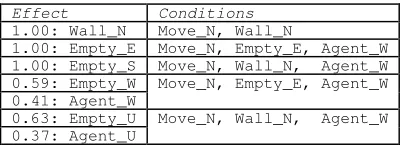
After steps 1 and 2 from section 2.5, we are left with the rules in Table 2 for the initial percept{Wall_N, Empty_E, Empty_S, Agent_W, Empty_U} and actionMove_N.
Table 2: Rules generated by the ASDD algorithm for the predator prey scenario matching an initial percept Wall_N,
Empty_E, Empty_S, Agent_W, Empty_U and action Move_N, after removal of rules by precedence.
Effect Conditions
1.00: Wall_N Move_N, Wall_N
1.00: Empty_E Move_N, Empty_E, Agent_W 1.00: Empty_S Move_N, Wall_N, Agent_W 0.59: Empty_W
0.41: Agent_W
Move_N, Empty_E, Agent_W
0.63: Empty_U 0.37: Agent_U
Move_N, Wall_N, Agent_W
Table 3: Generated states and associated probabilities from the rules in Table 2.
Wall_N Empty_E Empty_S Empty_W Empty_U 0.37 Wall_N Empty_E Empty_S Empty_W Agent_U 0.22 Wall_N Empty_E Empty_S Agent_W Empty_U 0.25
Wall_N Empty_E Empty_S Agent_W Agent_U 0.15
2.5.4 Precedence
Precedence (or deferral) between rules is required in situations where two or more rule-sets match the conditions for the same output variable. The state generator picks the rule-set which best matches the original data gathered from experience for the combined conditions. Table 4 and Table 5 show rules which both apply to the square to the north of the agent. In order to establish precedence in situations where both rule-sets conditions hold, the rule-set which best describes a rule with the combined conditions (Table 6) is preferred. In this example, we can see that the combined rule-set does not contain an agent to the north, so the set in Table 5 would be preferred.
In this case the rules in Table 5 state that we will not see an agent to the north if we move north and previously observed an agent to the south. This is correct because there is only one agent in the environment and it could not have moved to the north if it was previously observed to the south.
Table 4: Rule set with conditions: action = Move_N and percept contains Empty_N
Effect Conditions
0.6: Empty_N Move_N, Empty_N
0.1: Agent_N Move_N, Empty_N
0.3: Wall_N Move_N, Empty_N
Table 5: Rule set with conditions: action = Move_N and percept contains Agent_S
Effect Conditions
0.7: Empty_N Move_N, Agent_S
[image:6.612.74.277.114.187.2]0.3: Wall_N Move_N, Agent_S
Table 6: Rule set with combined conditions
Effect Conditions
0.75:Empty_N Move_N, Empty_N, Agent_S 0.00:Agent_N Move_N, Empty_N, Agent_S
0.25:Wall_N Move_N, Empty_N, Agent_S
3. RULE VALUE REINFORCEMENT
LEARNING
Section 2 described the use of rules to model an environment. The next task for the agent is to use this rule model to develop an effective policy for action in the environment. One method of achieving this is to use a standard reinforcement learning technique such as Watkins Q-Learning [14].
Reinforcement learning techniques feed back rewards (or costs) encountered in each state to the state which led to the reward. In Q-learning, each state-action pair is given a value, which represents the utility of taking the action in the state. If an agent has an accurate state-action map, it can then take the optimal action by choosing the highest valued action for that state.
The update function for Q-learning is as follows:
'
'
( , ) ( , ) [ s max ( ', ') ( , )]
a
Q s a ← Q s a + αR + γ Q s a − Q s a
(3.1)
Where s and a are the states and actions. s’ is the resulting state and a’ is the following action. Rs’ is the reward received for the following state. Q(s,a) indicates the current Q value for the state action pair. This update rule gradually improves estimates on the target function Q. The α parameter is a step-size, indicating how quickly the new estimate should change the old one. γ indicates the discount factor, determining the influence of future rewards on the current state.
If the agent continually follows an optimal policy (picks the best action at each stage) with some error introduced in order to allow it to explore, the Q-learning algorithm will converge on an optimal policy with a probability close to 1.0 [12]. If we use this function and take sample results (i.e. s’is taken to be the random result after taking action a in state s) the learning is one-step temporal difference (TD) learning.
= -1}. The values in column value (1) show the values after the sequence of actions and results below:
State: Heads, Action: Flip, Result: Heads State: Heads, Action: None, Result: Heads
The values for the column value (2) show the values after four further actions:
State: Heads, Action: Flip, Result: Tails State: Tails, Action: None, Result: Tails State: Tails, Action: Flip, Result: Heads State: Tails, Action: Flip, Result: Tails
Table 7: Example Q-Values for the coin flipping agent (α=0.5,
γ = 0.95). Rewards: {Heads=1, Tails=-1}
State Action Value(1) Value(2)
Heads Flip 0.5 -0.0125
Tails Flip 0 0.329
Heads None 0.738 0.738
Tails None 0 -0.5
3.1 The Rule Value Update Function
The Rule Value Reinforcement Learning (RVRL) method that we present in this work uses the same principle as TD learning to update a value associated with each rule, rather than each state. The main advantages of using a state-based aggregation method, such as RVRL, over a standard reinforcement learning technique are that:
a) The agent does not have to store a complete value-map with entries for every possible state-action combination in the environment.
b) The agent can generalize over many states, thus allowing one value to represent many states with similar properties, and allowing a sensible action to be taken in previously unseen states.
The coin flipping example can be used to demonstrate this technique. The conditions captured in our rule-set for calculation of next state reflect structural characteristics of the environment for calculation of a value-map. The rule values can be updated using the Q-learning equation, because there is only one output variable in each rule. Table 8 shows Q(Rule)
approximations for the coin flipping example using the sequence of actions and results used for
Table 7.
[image:7.612.309.565.96.164.2]The value of the flip action will be the same, whether the current state is Heads or Tails, and we can thus update the table more accurately.
Table 8: Example Q(Rule) Values for the coin flipping agent (α=0.5, γ = 0.95). Rewards: {Heads=1, Tails=-1}
Prob Effect Conditions Value(1) Value(2)
0.5 Heads
0.5 Tails
Flip 0.5 0.3231
1.0 Heads None,
Heads
0.738 0.738
1.0 Tails None,
Tails
0 -0.505
If a model of the environment is available, full backup values can be used. Rather than taking a random sample for st+1, the probability (P) of reaching each possible next state (s’) given that action a was taken in state s can be used in the equation, and the best next action taken as the maximum action (a’) for each possible next state. This is the principle behind dynamic programming (DP). The update function for DP [12] is:
' '
'
'
( , )
( , ) [ max ( ', ') ( , )]
a s ss
a s
Q s a
Q s a P αR γ Q s a Q s a
←
+ ∑ + −
(3.2)
The stochastic planning operators act as a model in rule value reinforcement learning: it is therefore possible to use an adaptation of the above equation.
The rule values for stochastic planning operators cannot be updated directly using equation (3.2), because more than one rule will match the next state (s’) and would therefore be used to generate consecutive states (see Table 2) due to several output variables being present.
The rule learning function, therefore, replaces
Q(s’,a’) with an average value for all matching rules which have precedence (and would therefore be used in generation of the successor state). The rules with precedence are used to give the most accurate representation of the dynamics of the environment in state s’.
( ) ( ) ' ' ' ' , ( ) ( )
[ max ( ( ', '))
( )]
a s
ss a
s
forEach rule MatchingRules s a
Q rule Q rule
R AvgQ WinningRules s a
Q rule
P
α γ∈ ← + + −
∑
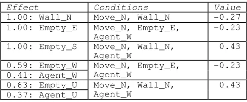
(3.3) [image:8.612.52.296.295.396.2]AvgQ(WinningRules(s’,a’)) returns the average rule value for rules which have precedence in state s’ if action a’ is taken. Table 9 shows the winning rules from Table 2 and the values that have been learned for them after 15,000 iterations of the rule update function. Notice that all rules with the same condition have the same value.
Table 9: Rule Values for a set of Winning Rules
Effect Conditions Value
1.00: Wall_N Move_N, Wall_N -0.27
1.00: Empty_E Move_N, Empty_E, Agent_W
-0.23
1.00: Empty_S Move_N, Wall_N,
Agent_W 0.43 0.59: Empty_W 0.41: Agent_W Move_N, Empty_E, Agent_W -0.23 0.63: Empty_U 0.37: Agent_U Move_N, Wall_N, Agent_W 0.43
AvgQ(WinningRules(s’,a’)) finds the average value of the winning rules and returns the value. The average value of the rules in Table 9 is: (-0.27 -0.23 +0.43 -0.23 +0.43)/5 = 0.026.
MatchingRules(s,a) returns all rules whose conditions match the current state and action. The values of all the returned rules are updated by equation (3.3).
3.2 Iterative Rule Value Evaluation
Section 2.5 described the process of building successor states using stochastic planning operators as a model. If this is combined with the rule-value update function given in equation (3.3) it is possible to continuously generate next states from an initial state and update the rule values for those states until satisfactory values for the rules have been generated (or a number of updates, n, has been performed). This process is described by the following algorithm:
Initialise Q(rule) = 0, for all rule ∈ rules; Repeat {
Initialise s = random state, a = random action; Generate next states, s’ and prob(s’) for s,a totalValue = 0; totalReward = 0;
For each s’ ∈ successor states { totalReward += reward(s’) * prob(s’); maxActionValue = -∞;
maxAction = null; For each a’ ∈ actions {
actionValue = AvgQ(WinningRules(s’,a’)); if (actionValue > maxActionValue)
maxActionValue = actionValue; }
totalValue += maxActionValue * prob(s’); }
For each rules ∈ matchingRules(s,a) Q(rule) = Q(rule) +
α[totalReward + γ*totalValue; –Q(rule)];
} for n steps
The sampling (TD learning) equivalent to this method would take a sample next state s’ rather than calculating the probability of each next state. The process is otherwise the same.
A low α value should be used in order to allow the rules to gradually approach the correct value, rather than being influenced by rules which do not directly correspond to reward states. In the predator prey environment, for example, reward values are based on whether the prey is the same square as the predator. Other rules may fluctuate greatly in value.
4. EXPERIMENTATION
RVRL as described in the previous section was applied to the predator-prey environment outlined in section 2.5.2. The task for our learning algorithm is to construct an effective policy under these conditions, allowing the predator to catch the prey with optimal frequency. The task is complicated by the fact that the predator is only adjudged to have captured the prey if the prey moves into, or remains in, the predator’s square at the end of its turn. Therefore the predator could not simply catch the prey by moving onto its square each move. The task is continuous, rather than episodic, meaning that the predator and prey will continue to move after the prey is caught, rather than re-starting each time.
tactic as the prey is then likely to move onto the predator and thus be caught. The optimal tactic, however, gained from a very large observation set (200,000 moves) was found to be one in which the predator moves into the prey’s square every move. This enables the predator to always be in sight of the prey and catch it whenever the prey moves into a wall. An example of a rule which captures this behaviour is one with the conditions:
Agent_N, Move_N.
Our experiments showed that RVRL gives high value to this rule and the Move_S, Move_E and Move_W
equivalents. Rules which attain higher value than this are more effective and have conditions such as:
Agent_U, Move_N, Wall_N, Wall_E
This corresponds to the situation where the predator is on-top of the prey in the NE corner of the map and chooses to move into a wall to the north. This gives the predator a 50% chance of catching the prey (the prey moves randomly and will move into the wall to the north or east 50% of the time). The “effects” of the rules are not shown, because the same value will be learned for all rules with the same conditions.
A sample of the final rule weights from rules learned from 60,000 moves experience after RVRL was run on the rule set for 15,000 iterations is given in Table 10.
Table 10: Sample rule weights for rules learned from 60,000 moves experience and 15,000 iterations of RVRL.
No. Conditions Value
1 Move_W, Wall_W, Wall_S, Agent_U 0.43
2 Move_E, Wall_W, Wall_S, Agent_U -0.03
3 Move_N, Wall_W, Agent_N 0.11
4 Move_N, Wall_N, Agent_U 0.11
5 Move_E, Agent_E -0.07
6 Move_W, Agent_E -0.21
7 Move_S -0.28
8 -0.28
Rules 1 and 2 have the same conditions, in that the predator is in the south west corner of the grid, with the prey underneath it. The rule has a positive value if the predator moves into a wall (rule 1), and a negative value if the predator moves away from the wall (rule 2). The agent would, therefore, pick the action of moving into the wall and thus have the highest chance of catching the prey (50% if the prey moves into a wall on its move).
Rules 3 and 4 both have the same weight. If the predator takes the move north action in rule 3, it will
be on-top of the prey and will therefore catch the prey if it moves into the wall to the west, which will happen 25% of the time. If the predator takes the move north action in rule 4 it will move into the wall and therefore stay on-top of the prey (which is under it). The predator will then catch the prey if it moves into the wall to the north, which will happen 25% of the time. These two situations should be of equal utility to the agent, which has been successfully learned by RVRL.
Rules 5 and 6 show the weights for moving east onto the prey to the east and moving west away from a prey to the east respectively. Moving onto the prey has a higher weight, and the predator will thus pick this action.
Rules 7 and 8 have the same value. Rule 7 is the general value of moving south with no other information. Rule 8 has no conditions and is thus the general value of taking a random move in the environment. These rules have the same value, which makes intuitive sense because moving south with no information would effectively mean taking a random move.
Tests were performed on the performance of Rule Value Reinforcement learning with:
a) Dyna-Q: a reinforcement learner which builds a frequency based model of the environment. Q-Learning is used on the acquired model to build values for each state action pair (the Q(s, a) map).
b) A stochastic rule based model of the environment to build a state, action value map. This is the equivalent of running Q-learning, using the rule based model for experience to build the Q(s, a) map. This method is described in [4].
Rule Value reinforcement learning builds a Q(rule) map, assigning value to each rule. Table 11 gives a comparison of the three methods.
prey was then recorded. The average number of moves taken to capture the agent is given in Table 11.
The two Q-learning based methods selected the best action at each step picking the highest valued action from all matching Q(s,a) values for the current state (s).
Rule based reinforcement learning picked the highest valued action from all matching:
AvgQ(WinningRules(s,a))
This was achieved by taking each possible action in turn and finding the value of:
[image:10.612.56.293.335.396.2]AvgQ(WinningRules(s,a)) for the current state (s).
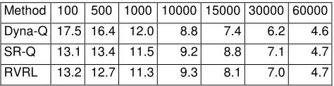
Table 11: Moves per capture for Dyna-Q, Stochastic Rule model Q (SR-Q) and Rule Value Reinforcement Learning (RVRL). Reinforcement learning ran for 15,000 iterations.
Trials ran for 40,000 steps. Training data gathered for between 100 and 60,000 steps
Method 100 500 1000 10000 15000 30000 60000
Dyna-Q 17.5 16.4 12.0 8.8 7.4 6.2 4.6
SR-Q 13.1 13.4 11.5 9.2 8.8 7.1 4.7
RVRL 13.2 12.7 11.3 9.3 8.1 7.0 4.7
Moves per capture for the predator taking random moves in the environment were found to be 16.01 (there are 16 squares is the environment and the predator will be randomly in the same 1 in 16 moves.
A trail was also run on a “perfect” model (a Dyna-Q model built from 400,000 moves). In this instance, the predator took 4.32 moves to capture the prey.
The results in Table 11 for 100, 500 and 1000 moves training data show that RVRL is more effective than Dyna-Q when very little experience has been gathered in the environment. In this case the Dyna-Q agent is forced to take a random move in many of the states encountered in the test, because it has no experience which matches the situation. An environment in which a random move was more costly would, therefore, show the value of RVRL in a more pronounced way under limited training data. With this limited model the Dyna-Q system “expected” the prey to move in the same way as it did in the training data, which often meant it picked an action that performed poorly. The RVRL agent, however, was able to make generalisations in two ways: first to generalise a model using the stochastic logic rules, which allows
the system to predict future states from the current state, even when this state has not been seen before; second, RVRL learned values are applicable across multiple states, allowing learned values to be applied in unseen states. This allows the small amount of experience gathered to be generalised and used, which is demonstrated by the improved performance under these conditions. SR-Q is only able to make use of the first of these generalisations, and therefore performed slightly better than Dyna-Q, but not as well as RVRL.
As the state action map gains a larger amount of experience (10,000, 15,000 and 30,000 steps), its model becomes closer to a perfect model in this test environment, while the generalisations made by the rule learner become less effective. This is due largely to shortcomings in the ASDD modelling method with this level of training data [4] which is reflected in the similar performance of the SR-Q results. The similar performance of SR-Q and RVRL shows that the slightly lower performance is due to this modelling inefficiency, rather than shortcomings in the RVRL algorithm. The increased performance of RVRL over SR-Q demonstrates that the ability of RVRL to generalise helps overcome this shortcoming.
When the learned rules become a near perfect representation of the environment (at 60,000 steps training data), the results show that RVRL is capable of learning near perfect valued rules, and thus the utility of taking an action in the current state, again demonstrating that the rule values are capable of capturing a policy at least as effectively as a state action model under these conditions.
5. CONCLUSIONS
This paper has presented the Rule Value Reinforcement Learning (RVRL) method for agents situated in stochastic environments. The method builds upon earlier work on learning stochastic planning operators, with emphasis on making these techniques applicable in agent-based systems. Results in our experimentation are extremely encouraging in that the algorithm is able to learn rule-values which accurately capture the utility of actions in the predator-prey environment without the need for a state-action map.
a) State-based aggregation;
b) Functional Approximation;
Techniques for reducing the need to store a number of state-action values exponential to the number of state variables in the state fall into two main categories: state-based aggregation and functional approximation. RVRL is a state-based aggregation technique, in that states which behave in a similar way with respect to a given action sequence and goal are given the same value. This type of aggregation is captured within the rule values in our technique. Other techniques in this category include:
a) Decision Theoretic Regression [2]: a decision tree representation of value is used, associated with a Dynamic Bayesian Network model of the environment. The method uses structure in the reward function to build a decision tree representation of the value-map which identifies regions of the state-action space whose values are the same. Regressions are made through each action to provide value trees for each available action.
b) Explanation based reinforcement learning [5]: Uses actions represented by deterministic STRIPS-like operators and has been extended to stochastic actions. Unlike RVRL, the technique does not allow for multiple concurrent output variables and assumes a single goal state rather than a general reward function.
Functional approximation techniques seek to create a compact approximation to the value function using, for example, neural networks. This technique gained prominence with TD-Gammon, which created a championship winning backgammon program [13]. The technique uses an approximation, rather than exploiting regions of uniform value in the feature space. Full comparisons with these techniques, however, are beyond the scope of this paper.
The use of acquired stochastic planning operators, combined with RVRL, represent a promising development in reinforcement learning. We plan to perform further tests in order to evaluate the performance of the method in a variety of environments. Scenarios in which the state variables are less tightly coupled are likely to show greater benefits for the method, compared to Dyna-Q based methods. These include the robot coffee-delivery
scenario, and process-planning problems presented in [2] which contain many more states than the predator prey problem, but can be compactly represented by factored state models. Other examples of test beds of this type can be found in [10].
6. REFERENCES
[1] Boutilier, C. and Dean, T. and Hanks, S.
“Decision-Theoretic Planning: Structural Assumptions and Computational Leverage”. Journal of Artificial Intelligence Research 11: 1-94, (1999).
[2] Boutilier, C., Dearden, R. and Goldszmidt, M. “Stochastic Dynamic Programming with factored representations”. Artificial intelligence, 121 (1-2), (2002).
[3] Child, C. and Stathis, K. “Rule Value Reinforcement Learning for Cognitive Agents”, Proceedings of AAMAS 2006, Hakodate, Japan (2006).
[4] Child, C. and Stathis, K. “The Apriori Stochastic Dependency Detection (ASDD) Algorithm for Learning Stochastic Logic Rules”, In Proceedings of the 4th International Workshop on Computation Logic in Multi-agent Systems (CLIMA-04), J. Dix, J. Leiter (Eds), Florida, Jan, (2004).
[5] Dietterich, T.G. and Flann, N.S “Explanation-Based Learning and Reinforcement Learning: A Unified View”. Machine Learning, 28, 169-214, (1997).
[6] Fikes, R.E. and Nilsson, N.J. “STRIPS: a new approach to the application of theorem proving to problem-solving”. Artificial Intelligence 2(3-4): 189-208, (1971).
[7] Kaelbling, L.P., Littman, H.L. and Moore, A.P.
“Reinforcement Learning: A Survey”. Journal of Artificial Intelligence Research 4: 237-285, (1996).
[8] Oates T., Schmill, M.D., Gregory, D.E. and Cohen P.R. “Detecting complex dependencies in categorical data”. Finding Structure in Data: Artificial Intelligence and Statistics V. Springer Verlag, (1995).
Planning with Incomplete Information for Robot Problems, AAAI, (1996).
[10]Pasula, H. M, Zettlemoyer, L.S. and Kaelbling, L.P. “Learning Probabilistic Relational Planning Rules.” Proceedings of the Fourteenth International Conference on Automated Planning and Scheduling, ICAPS, 73-82,(2004).
[11]Stathis, K., Child, C., Lu, W. and Lekeas, G. K. “Agents and Environments.” SOCS Technical Report IST32530/CITY/005/DN/I/a1, SOCS Consortium, (2002).
[12]Sutton, R.S., and Barto, A.G. “Reinforcement Learning: An Introduction”. A Bradford Book, MIT Press, (1998).
[13]Tesauro, G. J. “TD-Gammon, a self-teaching backgammon program, achieves master-level play.” Neural Computation 6, 2: 215-219, (1994).