Road Congestion

This is a repository copy of Road Congestion. White Rose Research Online URL for this paper: http://eprints.whiterose.ac.uk/91934/

Version: Accepted Version

Book Section:

May, A, Liu, R and Shepherd, S (2015) Road Congestion. In: Nash, C, (ed.) Handbook of Research Methods and Applications in Transport Economics and Policy. Handbooks of Research Methods and Applications Series . Edward Elgar , 112 - 133. ISBN

9780857937926

https://doi.org/10.4337/9780857937933.00013

[email protected] https://eprints.whiterose.ac.uk/ Reuse

Unless indicated otherwise, fulltext items are protected by copyright with all rights reserved. The copyright exception in section 29 of the Copyright, Designs and Patents Act 1988 allows the making of a single copy solely for the purpose of non-commercial research or private study within the limits of fair dealing. The publisher or other rights-holder may allow further reproduction and re-use of this version - refer to the White Rose Research Online record for this item. Where records identify the publisher as the copyright holder, users can verify any specific terms of use on the publisher’s website.

Takedown

If you consider content in White Rose Research Online to be in breach of UK law, please notify us by

Please cite this article in press as:

May, A.D., Liu, R. and Shepherd, S. (2015) Road Congestion, in Handbook on Research Methods in Transport Economics and Policy (ed. Nash, C), Chapter 6. Edward Elgar Publishing, ISBN 978 0 85793 792 6.

Handbook on Research Methods in

Transport Economics and Policy

Part 2 Externalities

Chapter 6: Road Congestion

Anthony D May, Ronghui Liu and Simon Shepherd

Institute for Transport Studies, University of Leeds, Leeds UK

1. Introduction

Every driver will have experienced the situation in which, as additional traffic joins a road, speeds fall, queues form and travel times become longer and more predictable. Engineers and traffic scientists have devoted considerable effort to understanding how such conditions arise, and how the key parameters of traffic flow, traffic concentration (or density) and traffic speed are related on individual roads (links) and in networks. This relationship, often referred to as the fundamental diagram of traffic, can be derived from first principles and from empirical evidence.

Economists and planners are more concerned with how to avoid the onset of congestion or to reduce its impact. This can be achieved in a range of ways, including enhancing capacity and managing the network better (both supply-side measures) and pricing, regulation and the provision of alternatives (which can be thought of as demand-side measures). In analysing them, economists need to understand both how the costs of travel are affected by travel demand (the supply curve) and how the demand for travel is influenced by the costs of travel (the demand curve).

Many early

are likely to be sensitive to temporal and spatial variations in demand, and discuss the policy implications.

2. The conventional economic analysis of supply and demand

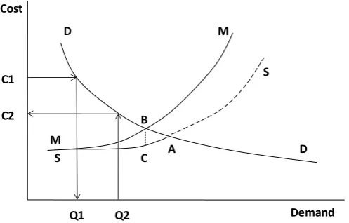
The prediction of traffic levels on an urban network requires determination of the intersection between demand and supply (Fig. 1). The demand curve D-D indicates the number of users (i.e. point Q1 in Fig. 1) for a given cost of using the facility (C1). Here Q is a function of C, as shown by the arrows. The supply curve S-S indicates how the cost of use (C2) increases as the number of users (Q2) increases. Here C is a function of Q, as shown by the arrows. The equilibrium level of usage is given by the intersection of the two curves (A). This is the user optimum, in which the nth user is just willing to incur the costs of travel which arise from there being n users. The part of the supply curve above the equilibrium is drawn as a dashed line to indicate that it is generally not observable, as discussed later in this chapter.

Note that when we speak of the cost of travel we are including the cost of the time taken; that is to say the amount of time multiplied by the value the user places on it. Ways of estimating such values are discussed in chapter 9.

The concept of congestion is loosely defined. However, congested conditions can be thought of as those in which the costs of travel are significantly increased by the interaction of other vehicles. We illustrate this further in the following section.

Q1 C2

C1

Q2 C

M

B

A

S D

Demand Cost

D S

M

Fig. 1 Standard model of supply-demand equilibrium, showing directions of causality.

For any such analysis, reliable estimates are needed of the shapes of both the demand and the supply curves. It will be clear from Fig. 1 that even small changes in their shape can have significant impacts on the estimate of usage and, even more so, on the estimated optimal road pricing charge. Both of these in turn will significantly influence the calculation of benefits. There is a substantial literature on the estimation of demand, as outlined in Chapter 10 (e.g. Bell, 1983; Ben-Akiva & Morikawa, 1990; Williams, 1977), which we take as given in this chapter (though we consider briefly how to define demand for a network). There has been much less discussion on the estimation of supply curves until recently (e.g. May et al, 2000; Small & Chu, 2003; Geroliminis & Levinson, 2009), and some economists have wrongly applied the fundamental diagram of traffic as an indication of the way in which costs rise as traffic levels increase.

We start by defining and deriving the fundamental diagram of traffic, reflecting the relationship between flow, concentration and speed, for a single link. We then consider how such relationships might be derived for networks. These diagrams reflect the

s on links and in

networks. We then consider the ways in which some economists have attempted to use such relationships to derive supply curves for links (and, by implication, networks), demonstrate that the fundamental diagram is inappropriate as a basis for estimating supply curves, and present alternative ways of doing so.

3. The fundamental diagram for single links

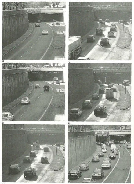
form, and traffic may be at a standstill for considerable periods. These six conditions are referred to in the Highway Capacity Manual (HCM, 2000) as levels of service A to F.

There are in practice two ways in which the number of vehicles can be counted on a road. One is illustrated by Figure 2. One can photograph a length of road x, count the number of vehicles nxin one lane of the road at a point in time, and derive a rate per unit distance. This

measure is called the concentration of traffic (sometimes referred to as density) and is denoted by the parameter k (veh/m). Thus

k=nx/x. (1)

The second approach is to stand at the side of the road for a period of time t, count the number of vehicles nt passing that point in one lane in that period, and derive a rate per unit

time. This measure is called the flow of traffic (sometimes referred to as volume) and is denoted by the parameter q (veh/s). Thus

q=nt/t. (2)

Since traffic engineers are concerned to get as many vehicles through a road as possible in a given time, they will wish to achieve as large a value as possible of q (rather than k), so capacity is described as the maximum value of q, qm. However it is not immediately clear

which of Figures 2a-f represents this condition.

While traffic engineers are concerned to achieve flows approaching capacity, individual drivers will be most concerned about the quality of their journeys, measured either by the speed at which they can travel or their travel time. Individual speeds (in m/s or km/h) are easy enough to measure, but in understanding traffic behaviour we need a measure of average speed. As shown elsewhere (May, 2001), the appropriate measure of speed is the space mean speed, us which can be measured by averaging the speeds of individual vehicles

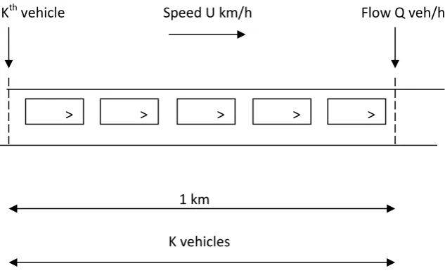
Figure 3. A simple derivation of the relationship between concentration, flow, and speed.

For any given stable traffic condition, the three parameters k, q and u are directly related. This can be seen from the simple example in Figure 3, which considers a kilometre of road, on which all vehicles are travelling at the same speed. The parameters K, Q and U are concentration in veh/km, flow in veh/h, and speed in km/h, respectively. By definition there are K vehicles, each with speed U, in the kilometre of road at any instant. If the flow is recorded at the end of the road, Q vehicles will pass per hour. The vehicle at the start of the kilometre will take1/U hours to reach the end at a speed of U km/h. It will then be the Kth vehicle to pass the end of the road, and this will happen in K/Q hours. Thus

1/U = K/Q or Q = KU. (3)

This is dimensionally correct, viz., veh/h = (veh/km)(km/h).

The same expression using metres and seconds, is

q = ku. (4)

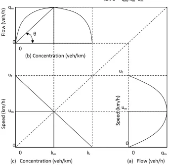
While equation (4) is important, it is still necessary to know the values of two of the parameters in order to calculate the third. In practice, on a given road, a given concentration is likely to give rise to a certain value of flow and a certain value of speed, subject always to the variations in driving conditions and driver behaviour. This relationship can best be seen by considering the three parameters a pair at a time, as in Figure 4. In each of them there are two limiting conditions, which can be thought of by reference to Figures 2a and f.

> > > > > Speed U km/h

K vehicles Kth vehicle

1 km

In figure 2a flow is very low (approaching zero), and so is concentration; the speed, which is likely to be at its highest, is referred to as the free flow speed uf. In Figure 2 if the speed is

zero and so, since the traffic is not moving, is the flow; however, the concentration is at its highest , and is referred to as the jam concentration kj.

Figure 4. Flow-concentration, speed-flow, and speed-concentration curves.

Figures 4a and 4b illustrate that as speed falls from uf to zero, and as concentration rises

from zero to kj, flow first increases and later falls again to zero. It seems reasonable to

expect that it only rises to one maximum, and this can be thought of as the capacity qm. As

flow increases towards capacity it is relatively easy to understand what is happening; as Figures 2a-e show, vehicles increasingly disrupt one another, reducing the driver s ability to choose his/her own speed or overtake others. Speed thus falls and concentration increases. Beyond capacity it is less easy to explain what is happening. In practice such conditions are caused by queues from downstream conditions, perhaps a junction or an accident or even a gradient or tight curve whose capacity is slightly lower. The queue leads to increased concentration; speeds fall further, and vehicles which cannot flow past the point join the queue as it stretches upstream. This situation is characteristic of bottlenecks on individual

uf

m/Km=um

(b) Concentration (veh/km)

(c) Concentration (veh/km) (a) Flow (veh/h)

F

lo

w

(

ve

h

/h

)

S

p

e

e

d

(

km

/h

)

S

p

e

e

d

(

km

/h

)

0 0

0

0 0

0

km kj qm

qm

um

uf

roads, and demonstrates clearly how congestion, in which concentration is high and speed and flow low, can be generated.

Several analysts have attempted to fit relationships to observed data. This is most easily done with concentration and speed (Figure 4c), since the relationship is monotonic. However, care needs to be taken in manipulating data to fit such a relationship (Duncan, 1979). The most common relationship, shown in Figure 4c, is a linear relationship between speed and concentration, as first suggested by Greenshields (1934):

u = a + bk. (5)

Using the two limiting conditions, it can be shown that this becomes

u = uf(1 - k/kj). (6)

Other analysts have noted from empirical data that the relationship is not quite linear but slightly concave. They have suggested logarithmic and exponential alternatives (Greenberg, 1959; Underwood, 1961). Each of these relationships has been supported by theoretical analysis, primarily based on an analogy with fluid flow (Lighthill and Whitham, 1955) and the interpretation of car-following behaviour (Herman et al., 1959). However, it is important to stress that traffic flow is not a wholly scientific phenomenon, but one which depends on the vagaries of driver behaviour. Indeed, some authors have suggested that there is no reason why conditions above and below capacity should be part of the same relationship, since they arise in different ways (Edie, 1961; Hall and Montgomery, 1993).

4. The fundamental diagram for networks

possible that other traffic movements will have restricted the performance of the upstream junction, resulting in a flow much lower than capacity, and relatively high speeds.

All of these considerations make the analysis of urban networks far more complicated than that for individual links, and there have been far fewer attempts to consider them. As a generality, performance will depend on

(1) the shape of the network; (2) the type of traffic control; (3) the controls on individual links;

(4) the pattern of journeys through the network (through versus terminating; short versus long; radial versus orbital); and

(5) the overall level of demand.

Similar relationships to those of Greenshields and Greenberg have been shown, from empirical observations, to be present at the network level in traffic flows which are regularly interrupted by junction controls in urban networks. Thomson (1967) developed a linear speed-flow relationship from data collected from the streets in central London over many years. Godfrey (1969) found a parabolic relationship between average journey speed and network vehicle km travelled in the network in central London, and showed that the speeds are inversely proportional to the concentration (defined as the number of vehicles in the network in central London at a given time). Examining data from urban networks in England and the US, Zahavi (1972) found that the average speed is inversely proportional to flow.

Theories of such area-wide relationships have also been proposed, e.g. in the seminal work of Smeed (1966) and by Wardrop (1968) who proposed a monotonically decreasing relationship between average speed and flow in a network. Later, Herman and Prigogine (1979) and Herman and Ardekani (1984) proposed a two-fluid model that allows for a more realistic representation of the congested part of the diagram. Mahmassani et al. (1987) presented a theoretical framework for the generation of network-level fundamental diagrams from simulation models.

More recently, significant developments have been made by Daganzo and colleagues with a series of theoretical developments and empirical verifications. They presented a theoretical

D

Implied capacity

Free-flow

Speed (km/h)

Flow (veh/h) C

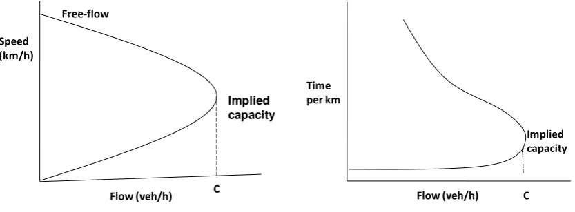
5. S application of the fundamental diagram

A typical relationship between space mean speed and traffic flow is thus as shown in Fig. 5a. As Small and Chu (2003) noted, Walters (1961) was the first to propose the standard way in which economists began to think about congestion. He transformed the fundamental diagram for a single link into a relationship between travel time and flow (as in Fig. 5b) and suggested that this represented an average cost curve for that link. the network. But the non-unique relationship between travel time and flow caused him and subsequent economists problems. As shown in Verhoef (1999), it is possible for the demand curve to intersect the average cost curve three times. Walters suggested that an equilibrium point in

ists since have

“ C

Some economists, including Else (1981), Hau (1998), Verhoef (1999) and Ohta (2001) have spent some time discussing the meaning of equilibrium points in the upper part of the curve, even though Newbery (1990) had warned that these were unstable conditions which were unlikely to represent dependable equilibria. Others, including Morrison (1986) and Evans (1992) have suggested that this part of the curve is irrelevant, and have simply removed it from their analyses.

More recently, economic analysis has been based on a bottleneck model, which more fully reflects the effects of queues in networks (Arnott et al, 1990) and it is this approach which is adopted by Proost in Chapter 13.

Fig. 5 Parabolic speed-flow curve for a link (a) and its inverse (b).

In practice, as we have argued elsewhere (May et al, 2000), the fundamental diagram is inappropriate as a means of determining the supply curve. It is an engineering performance curve, which represents how the facility performs given observable flows in a given time period. (In practical applications, such curves have been observed, or modelled, for periods of between 15 minutes and an hour, in which conditions can be expected to be reasonably

Implied capacity Time

per km

stable.) However, what is needed for a supply curve (such as SS in Fig. 1) is an estimate of the time which would be spent by the demanded flow, at each of a given set of increasing levels of demand, up to the point where that demanded flow leaves the facility. At low levels of demand, when there is little or no congestion, the performance curve will provide a reasonable estimate of the time taken, since journeys can be expected to be completed in the time period represented by the performance curve. However, in congested conditions in which journeys take some time, the travel time experienced will be influenced by the

one location to another. Moreover, if it is to be used to assess equilibrium under a range of possible future demand levels, a supply curve has to be able to indicate the travel times which would occur at demand levels higher than those which currently occur on the network (as indicated by the dashed curve in Fig. 1), which are hence unobservable.

A separate strand of exploration has concerned the meaning of demand. Neuberger (1971) was the first to point out that, in a single link, the flow entering a link represented demand, while the flow leaving it represented supply, and that in congested conditions the two would differ. Unfortunately his observation was largely ignored by others. Even this distinction needs to be defined more carefully when dealing with an urban network. Users can no longer be thought of as simply demanding flow. As Hills (1993) points out, they demand trips, but those trips will differ in length and orientation, and some will terminate within the network. May et al (2000) used vehicle-km in the network as a simple representation of demand.

Hills (2001) argued that a supply curve for a network would involve some sections which are congested and others which are not, and that this would lead to a monotonically increasing supply curve. While it is indeed true that not all roads in a given network will be congested,

this will be fundamental diagram, and hence its performance

curve. But as congestion increases, drivers will take longer to travel through the congested area, and will experience conditions outside the space-time domain for which a given performance curve has been drawn.

This is illustrated in Fig. 6, in which each vehicle is represented by a trajectory in time and space, and the slope of the trajectory falls as congestion increases. A typical performance curve (or fundamental diagram) is derived for a rectangular space-time domain ABCD, and includes the impact of some drivers who start before the time period, some who complete their journeys within it, and some who have not completed their journeys by the time that it ends. It is clear from Fig. 6 that this does not represent the time incurred by those drivers who start their journeys in the time period AB. To do this, and hence derive a supply curve, we need a quadrilateral time- ABC D F 6. This was the approach which we adopted in our earlier work (May et al, 2000), and which was accepted

recent authors continue to argue that performance curves should be used in preference to supply curves to estimate the costs of congestion. Geroliminis and Levinson (2009) suggest

that supply curves . . .

account of the time-dependent nature of congestion. As we illustrate below, it is possible to develop supply curves which reflect variations in demand in both time and space.

Fig. 6 Space-time domains for MFD and supply costs.

6. An analysis of the nature of network supply curves

In recent research, we have used a micro-simulation model (Liu et al. 2006; Liu, 2010), and simplified networks representing the cities of Cambridge and York in the UK, to determine the shapes of network performance and supply curves differences between them and, in particular, whether the shape of the supply curve is sensitive to the temporal and spatial distribution of demand. For these purposes we have used matrices which reflect the current pattern of demand in each city, distributed uniformly over the morning peak period, and also ones which vary that demand over time and space. Each demand matrix was factored to give a series of levels of demand, which represent the points in the curves shown in the following section, and which allow us to understand the shape of the supply curve at levels of demand higher than those which are currently observable. We summarise the methodology here and the results in the following section. Fuller detail is provided in Liu et al (2011).

As indicated in Fig. 6, performance curves are based on measurements of vehicle-km/hour and vehicle hours/hour in a network, averaged over a given time period, and can be used to estimate the network equivalent of speed-flow curves or network fundamental diagrams. These parameters can be measured and have been used by earlier authors to describe the way in which costs of using the network rise as usage increases as reviewed above. Again, as indicated in Fig. 6, in order to calculate average costs per trip for a supply curve, individual

Space

A

C

B

D D’ C’

Trajectory of first vehicle generated in AB

Trajectory of last vehicle generated in AB

Generating period AB (g) O

v

in the network at a given point in time.

Moreover, in order to determine a full supply curve, estimates are needed of the unit costs which would be incurred across the full range of demand levels, from those consistent with free flow to those related to congestion approaching gridlock. Without such values, it is not possible to determine the intersection between the supply and demand curves if, for example, exogenous factors lead to an increase in demand. Since it is precisely at the points of intersection of the average and marginal cost curves with the demand curve that the economic implications of a particular policy are determined, it is particularly important that the supply curve is specified and estimated correctly in these conditions. But, as illustrated in Fig. 1, the conditions resulting from higher levels of demand cannot be observed. This implies that empirical observation, even if vehicles could be tracked to determine their costs, would not be a sufficient way of obtaining all the data needed. It is for these reasons that we have employed micro-simulation to derive both performance and supply curves.

As a simplification of the approach which we adopted in May et al, 2000, we have described demand in terms of vehicle trips in a given period. As noted above, a vehicle-trip may have a different impact on the network, and experience different costs, depending on its length and orientation within the network, the route taken, the time at which it occurs and the overall level of demand. If this hypothesis is correct, demand in trips needs to be associated with a given spatial and temporal matrix shape and the results obtained will be relevant only for that matrix. For any matrix, the effects of increased demand can then be reflected by increasing the total number of trips, while maintaining the same spatial and temporal distribution. The impact of demand on the network is, in practice, modified by two particularly important behavioural responses by drivers: re-routeing and rescheduling. In our research, we considered the re-routeing effect only.

The one exception to the use of trips to measure demand is in the comparison of supply and performance curves (in Fig. 9 below). There, since performance curves relate time per km to veh-km/h, we use the same units to measure supply, so that the curves can be directly compared. In doing so, we use actual km travelled, which will be affected in part at higher levels of demand by re-routeing. We also use time per km in Fig. 13b, in which we compare different origin-destination movements of differing lengths.

7. Empirical results

Performance and supply curves

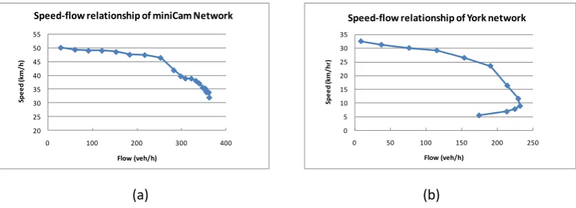
Fig. 7 shows the speed-flow curves as simulated for the C miniCam and York networks respectively over the one-hour generation period. In this and in subsequent figures, each point represents a different level of demand over the generating period.

The speed-flow curve for the Cambridge network suggests that a maximum performed flow is reached with a speed of around 30 km/h (Fig. 7a). That for the York network (Fig. 7b) shows that the performed speed decreases with increasing flow up to a flow level of around 230 veh/h. From then on, the flow and speed both decrease as the demand increases.

(a) (b)

Fig. 7 The speed-flow relationships for the Cambridge network (a) and the York network (b).

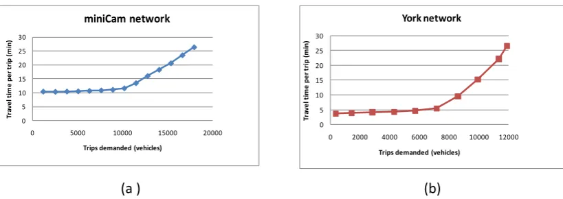
Fig. 8 shows the network supply relationships for the Cambridge and York networks. In both cases the trip journey time increases monotonically with the demand, measured as described above as trips in a given period.

As an alternative, which permits more direct comparison with the performance curves, these supply curves can be redrawn to show the relationship between time per km and vehicle-km demanded. Fig. 9 shows the relationships between time per km and the total vehicle-kms travelled (or demanded) for both the performance measure and the supply measure. For both networks, it shows a difference between the two relationships at higher demand levels. Whilst the performance curve, at least for the York network, is backward

T

that supply curves differ from performance curves, particularly above flow levels at which congestion begins to be experienced.

20 25 30 35 40 45 50 55

0 100 200 300 400

S p e e d ( k m / h ) Flow (veh/h)

Speed-flow relationship of miniCam Network

0 5 10 15 20 25 30 35

0 50 100 150 200 250

S p e e d ( k m / h r) Flow (veh/h)

(a ) (b) Fig. 8 The simulated supply curves for the Cambridge and the York network.

(a) (b)

Fig. 9 Comparison between the performance and supply measures for the two networks. Sensitivity of supply curves to temporal demand

In this test, using the Cambridge network, two alternative assumptions are made about the temporal demand distributions: one uniform (flat) over the one-hour period and one peaked with two 15-min periods in the middle with a demand level 1.3 times the average,

erage demand.

Fig.10 shows the supply curves aggregated over the one-hour demand period for the two demand profiles. It is clear that the peaked demand profile has induced much higher costs for a given level of demand (in trips in a given period) than those for the flat demand distribution. This is an expected result, but it illustrates the need for supply curves to be based on the correct temporal distribution of demand.

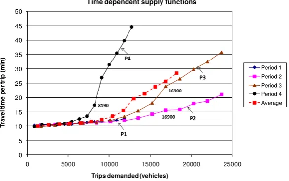
We can also see how the supply functions vary from one time period to another. Fig.11 shows supply curves for each of the four 15-min sub-periods with the peaked demand distribution, compared with that of the whole one-hour demand. It shows the cost per trip in a given demand sub-period as demand in that period increases. It can be seen that period 3 has higher costs for a given level of demand (in trips in a given period) than period 2, and that period 4 has higher costs than period 1. This is due to extended queues being passed from period 2 to period 3, and from period 3 to period 4. These results suggest that the supply costs vary during the peak hour, with congestion costs for traffic entering during the

0 2 4 6 8 10 12 14

0 5000 10000 15000 20000 25000

T ra v e l ti m e p e r k m ( m in ) Veh-kms York network Supply Performance 0 0.5 1 1.5 2 2.5 3 3.5 4

0 50000 100000 150000

T ra v e l ti m e p e r k m ( m in ) Veh-kms miniCam network Supply Performance 0 5 10 15 20 25 30

0 2000 4000 6000 8000 10000 12000

T ra v e l ti m e p e r tr ip ( m in )

Trips demanded (vehicles) York network 0 5 10 15 20 25 30

0 5000 10000 15000 20000

T ra v e l ti m e p e r tr ip ( m in )

most congested periods (Periods 2 and 3) being experienced by traffic entering in a later period (Period 4) even though the demand in Period 4 is lower.

Fig. 10 Supply curves for a flat- and a peak-demand profile for the miniCam network.

Fig. 11Supply functions of the miniCam network with a peaked demand profile for each of the four 15min time periods and the one hour average. The data points for period 1 coincide with those of period 2 and 3 up to the demand level of 12000 veh, so are not clearly visible in the plot.

Sensitivity of supply curves to spatial demand

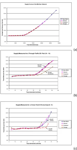
In this test, using the Cambridge network, the demand matrix was varied by increasing certain movements by 20% to illustrate the spatial effect on supply cost. Fig. 12 shows the simulated supply relationships for four different matrices (Fig. 12a), and for selected O-D movements under different matrices (b and c). The results suggest that at the aggregate level all total network-wide supply curves are similar i.e. the changes in matrix have no significant impact on the supply measures at an area-wide level. However, this is not always reflected at the level of individual O-D movements. For three of the selected O-D pairs (the Inbound, External-to-urban and Outbound), the matrix variation has no significant effect on the supply curves. However, for the Cross-Town O-D pair and the Through-Traffic O-D pair, the travel times per trip for a given level of demand (in trips in a given period) were lower

0 5 10 15 20 25 30 35 40 45 50

0 5000 10000 15000 20000 25000

T ra v e l t im e p e r tr ip ( m in )

Trips demanded (vehicles)

Time dependent supply functions

Period 1 Period 2 Period 3 Period 4 Average P1 P2 P3 P4 8190 16900 16900 0 5 10 15 20 25 30

0 5000 10000 15000 20000

T ra v e l ti m e p e r tr ip ( m in )

Trips demanded (vehicles)

miniCam network

flat

when that movement within the matrix is increased (b and c). This implies that the supply curves, for those O-D movements at least, are dependent on the shape of the demand matrix. It may well be that larger changes in the demand matrix would have demonstrated similar results for other O-D movements.

(a)

(b)

(c)

Fig. 12 The supply curves for the miniCam network: (a) for the total network under various demand

T -T O-D pair under four different demand matrices, and (c) and for a Cross-Town O-D pair under the four matrices.

0.00 5.00 10.00 15.00 20.00 25.00 30.00 35.00

0 10 20 30 40 50 60 70 80

T ra v e l t im e p e r tr ip ( m in )

Trips demanded (vehicles)

Supply Measures for a Cross-Town O-D Journeys (5 - 9 )

Base Matrix Inbound Crosstown Through Cross 60 vehicles Base 60 vehicles 0.00 5.00 10.00 15.00 20.00 25.00 30.00 35.00 40.00 45.00

0 20 40 60 80 100 120 140 160

T ra v e l t im e p e r tr ip ( m in )

Trips demanded (vehicles) Supply Measures for a Through-Traffic OD Pair (16 - 14)

Base Matrix Inbound Crosstown Through Through 120 vehicles Base 120 vehicles 0.00 10.00 20.00 30.00 40.00 50.00 60.00

0 5000 10000 15000 20000 25000 30000

A v e ra g e tr a v e l ti m e p e r tr ip (m in )

Trips demanded (trips) Supply Curves of the MiniCam Network

Sensitivity of supply curves to type of movement

Finally, Fig. 13a shows the differences in supply curves by OD movement types for the same base matrix as demand is increased. As might be expected, the longer Through and External trips have higher free-flow travel times than the other three movements. It can then be noted that as demand is increased, the supply relationships differ in terms of the increases in congestion experienced. The Through and External trips are the least readily congested. Conversely, the Outbound trips and Cross-town trips become congested at the lowest levels of demand, and unit travel costs for these movements increase most rapidly. Perhaps surprisingly (and somewhat counter intuitively), the Inbound trips are less readily congested than Outbound ones.

Comparing different OD movements of different lengths and travel times, it is perhaps desirable to examine the supply measure by unit distance travelled. Fig. 13b therefore shows the supply curves in terms of the average travel time per km travelled against the demanded trips. It can be seen that all five OD movement types have similar per-km free-flow travel times, but they all then exhibit very different supply curves as congestion sets in.

The supply curve for the Through traffic in Fig. 13b shows a slight dip in travel time per km at a demand level around 70. This is due to the effect of adding a new route, a longer route along the ring road, to this OD pair starting at this demand level.

(a) 0.00

20.00 40.00 60.00 80.00 100.00 120.00

0 50 100 150 200 250 300 350

T

ra

v

e

l t

im

e

p

e

r

tr

ip

(

m

in

)

Trips demanded (vehicles)

Supply curves for different OD pairs - travel time per trip

(b)

Fig. 13 Comparison of the supply measures for different O-D movements in the miniCam network under the same (base) matrix, measured in: (a) travel time per trip and (b) travel time per km travelled.

8. Estimation of supply curves

It must be recognised that it is not generally possible to observe costs (or travel times) for that part of the supply curve above the currently experienced number of trips (as indicated by the dashed line in Fig. 1) since, by definition, those conditions do not occur. Yet it is precisely these costs which need to be estimated to reflect the effects of increases in demand, such as those which might occur if an alternative mode became less attractive.

We envisage two ways in which these unobserved parts of a supply curve might be estimated. We have used microsimulation in our approach, and have shown it to work, although this method is dependent on the quality of the microsimulation model. New surveillance and communication technologies, such as GPS and GSM (global systems for mobile communication), allow the continuous tracking of the progression of vehicles. These

technologies and new data sources allow us to obser

curve. As an alternative, it may therefore be possible to develop functional relationships which allow the supply curve to be extrapolated from its observable part (shown as the solid curve in Fig. 1) to its unobservable part (the dashed curve). For example, in a functional relationship similar to that proposed by Vickrey (1969), we may formulate C = A + B(T/T0)k,

where C is the travel time per trip, T the total number of trips demanded, and A, B and k are constants which can initially be estimated from fitting the function to the observed part of the curve. Indeed, it may be that a combination of the two approaches would allow the extrapolation to be estimated using microsimulation, while the empirical data is used to validate the microsimulation at lower levels of demand.

0.00 2.00 4.00 6.00 8.00 10.00 12.00 14.00

0 50 100 150 200 250 300 350

T

ra

v

e

l t

im

e

p

e

r

k

m

(

m

in

)

Trips demanded (vehicles)

Supply measures for different OD pairs - travel time per km travelled

Cross-town Outbound Inbound External Through traffic

Given the findings above on the sensitivity of supply curves, it appears necessary to develop supply curves separately for different time periods and different movement types and, potentially, for different spatial distributions of the matrix.

9. Conclusions and implications for policy

Traffic conditions on a single link can be defined in terms of the flow, concentration and speed of traffic. These three parameters are related, in what is often referred to as the fundamental diagram of traffic. Analysis from first principles and empirical evidence both demonstrate that conditions vary between the two extremes of very light flow, with high speeds, and stationary traffic. Somewhere between these two extremes lies the condition in which traffic flow is maximised. Once demand exceeds this level, congestion increases, speeds fall and travel times rise substantially. Similar fundamental diagrams can be derived for traffic in networks, though the definition of parameters is more complicated.

Many economists have used such fundamental diagrams to develop supply curves which relate the cost of using a link or network to the level of demand for that link or network. However, as Fig. 9clearly illustrates, the fundamental diagram of a road network cannot be used in this way to estimate supply curves. The application of performance curves to estimate levels of usage is likely, in congested conditions, to under-estimate actual usage, and grossly to under-estimate the costs of the resulting congestion and the benefits of user charges to relieve congestion. Instead, supply curves need to be used for estimating demand. They cannot be observed throughout their range (as demonstrated in Fig. 1) and need instead to be estimated using the methods suggested in the previous section.

Performance curves do, however, have an important role in understanding how to improve the effectiveness of urban networks. The use, in Singapore, of speed thresholds as a basis for determining when charges should be raised or lowered, is a practical example of the effective application of performance curves.

The evidence that supply curves are dependent on the temporal distribution of demand has important implications for policy. In equity terms, it is clear that those using the network at certain times impose greater costs than others, and thus potentially merit higher charges. In network management terms, it is clear that congestion can be reduced more effectively by selective control of traffic levels in certain time periods.

terms, it appears appropriate to impose higher charges on those movements which are most readily congested.

In terms of policy stability, the fact that changes in the distribution of demand in time and space can influence the appropriate policy response implies that policy needs to be reviewed regularly, rather than simply assuming that a demand management measure, once applied, will continue to be effective. This has particular implications for land use policy. A large development in a given location will add to certain temporal and spatial movements, and could significantly affect the shapes of their demand and supply curves, thus justifying substantial changes in the demand management measures applied.

All the above remarks demonstrate the need for care in selecting a modelling approach when considering the impacts of policy on demand. When demand exceeds capacity, the dynamics imply the need for some form of dynamic model. Whilst most four stage static models can be used with multiple time periods and a departure time choice model, most do not deal adequately with the issue of queue pass-over from one period to the next. By their very nature they are based on the principles of steady-state systems within each time period. Instead it will be preferable to employ dynamic traffic assignment models (see a review in Peeta & Ziliaskopooulos, 2001), or the micro-simulation approaches as used in the study reported above.

While micro-simulation models are well developed in representing supply factors, further work is needed to fully integrate the spatial distribution of the O-D matrix (trip-patterns), the temporal distribution of the O-D matrix (trip-profiles), rescheduling in response to cost changes, and re-routeing in response to cost changes. Whether dynamic traffic assignment models or micro-simulation approaches are used, supply curves should be generated separately for different time periods and movement types if the models are to be integrated within a full supply-demand framework. Further work is needed to provide guidance on the appropriate degree of temporal and spatial differentiation for a given network and set of policy options.

Acknowledgements

We thank Elsevier for permission to extract the text and to reprint Figs. 1 and 5-13, from Transportation Research Part A, Vol L O

-965, Copyright (2011) Elsevier.

References

Arnott, R., de Palma, A. and Lindsey, R. (1990), Economics of a bottleneck Urban Economics, 27, 111 130.

Bell, M.G.H. (1983), The estimation of an origin destination matrix from traffic counts

Transportation Science,17 (2), 198 217.

Ben-Akiva, M. and Morikawa, T. (1990), Estimation of travel demand models from multiple data sources , in Kosji, M. (ed.), Proceedings of the 11th International Symposium on Transportation and Traffic Theory, Yokohama, July 1990, pp. 461-476.

Bird R.N. (2001) Junction design , in Button, K.J. and Hensher, D.A. (eds), Handbook of Transport Systems and Traffic Control, Oxford: Elsevier, pp. 399 412.

Daganzo, C.F. (2007), Urban gridlock: macroscopic modelling and mitigation approaches

Transportation Research Part B, 31 (1), 49 62.

Duncan, N.C (1979), A further look at speed/flow Traffic Engineering and Control, 20

(10), 482 483.

Edie, L.C. (1961), Car following and steady state theory for non-congested traffic Operations Research, 9, 66 76.

E P K A reformulation of the theory of optimal congestion taxes Journal of Transport Economics and Policy, 15, 217032.

Evans, A.W. (1992), Road congestion: the diagrammatic analysis Journal of Political Economy, 100, 211 217.

Geroliminis, N. and Daganzo, C.F. (2007), Macroscopic modelling of traffic in cities , in TRB 86th Annual Meeting, #07-0413m Washington, DC.

Geroliminis, N. and Daganzo, C.F. (2008), Existence of urban-scale macroscopic fundamental diagrams: some experimental findings Transportation Research Part B, 42, 759 770. Geroliminis, N. and Levinson, D.M. (2009), Cordon pricing consistent with the physics of

overcrowding , in William, L., Wong, S.C. and Lo, H.K. (eds), Transportation and Traffic Flow Theory, pp. 219 240.

Godfrey, J.W. (1969), The mechanism of a road network Traffic Engineering and Control, 11 (7). Greenberg, H. (1959) A Operational Research, 7 (1), 79 85.

Greenshields, B.D. (1934), A study of traffic capacity Proceedings of the Highway Research Board,

14, 448 477.

Hall, F.L. and Montgomery, F.O. (1993) The investigation of an alternative interpretation of the speed flow relationship on UK motorways Traffic Engineering and Control, 34 (9), 420 425. Hau, T.D. (1998), Congestion pricing and road investment Button, K.J. and Verhoef, E.T. (eds),

Road Pricing, Traffic Congestion and the Environment: Issues of Efficiency and Social Feasibility, Cheltenham, UK and Lyme, NH, USA: Edward Elgar Publishing, pp. 39 78.

HCM (2000) Highway Capacity Manual. Transportation Research Board.

Herman, R. and Ardekani, S.A. (1984), Characterizing traffic conditions in urban areas

Transportation Science, 18 (2), 101 40.

Herman, R., Montroll, F.W., Potts, R.O. and Rottery, R.W. (1959) T

Operations Research, 7 (1), 86 106.

Hills, P.J. (1993), Road congestion pricing: when is it a good policy? A comment , Journal of Transport Economics and Policy, 27, 91 99.

Hills, P.J. (2001), Characterisation of the Supply/Demand Interaction for an Urban Road Network Subject to Congestion, Chapter 2, Project PPAD/9/84/30: Analysis of Congested Networks, Department for Transport, UK.

L M J W G B O II A

crowded roads, Proceedings of the Royal Society A: Mathematical, Physical and Engineering Science, 229(1178), 317-345.

Liu, R. (2010), Traffic simulation with DRACULA Barcelo J. (ed.), Fundamentals of Traffic Simulation, pp 295-322.Springer.

Liu, R., May, A.D. and Shepherd, S.P. (2011), On the fundamental diagram and supply cost of congested urban networks Transportation Research Part A, 45 (9), 951 965.

Liu, R, Van Vliet, D. and Watling, D. (2006) Microsimulation models incorporating both demand and supply dynamics Transportation Research Part A, 40, 125 150.

Mahmassani, H., Williams, J.C. and Herman, R. (1987), Performance of urban traffic networks n

Proceedings of the 10th International Symposium of Transportation and Traffic Theory, Gartner, N.H. and Wilson, N.H.M. (eds), pp. 1 21.

May, A.D. (2001), Urban traffic flow , in Button, K.J. and Hensher, D.A. (eds), Handbook of Transport Systems and Traffic Control, Oxford:Elsevier, pp. 425 438.

May, A.D., Shepherd, S.P. and Bates, J.J. (2000), Supply curves for urban road networks Journal of Transport Economics and Policy, 34 (3), 261 290.

Morrison, S.A. (1986), A survey of road pricing Transportation Research, 20A, 87 98.

Neuburger, H. (1971) The economics of heavily congested roads , Transportation Research, 5, 283 293.

Newbery, D.M. (1990), Pricing and congestion: economic principles relevant to pricing roads

Oxford Review of Economic Policy, 6, 22 38.

Ohta, H. (2001) Proving a traffic congestion controvers Journal of Regional Science, 41, 659 680.

Peeta, S. and Ziliaskopoulos, A.K. (2001) Foundations of dynamics traffic assignment: the past, the present and the future Networks and Spatial Economics,1 (3 4), 233 292.

Quinn, D.J. (1992) A review of queue management strategies Traffic Engineering and Control,33

(11).

Sheffi, Y. (1985), Urban Transportation Networks, New Jersey: Prentice Hall.

Small, K.A. and Chu, X. (2003), Hypercongestion , Journal of Transport Economics and Policy, 37 (3), 319 352.

Smeed, R.J. (1966), ‘ Traffic Engineering and Control,8 (7), 455 458. Thomson, J.M. (1967), Speeds and flows of traffic in central London Traffic Engineering and

Control, 8 (12), 721 725.

Underwood, R.T. (1961), “ Quality and Theory of Traffic Flow; Bureau of Highway Traffic, Yale University, New Haven; pp. 141-187.

Vickrey, W. (1969), Congestion theory and transport investment American Economic Review, 59, 251 260.

Walters, A.A. (1961), The theory and measurement of private and social cost of highway congestion Econometrica, 29, 676 699.

Wardrop, J.G. (1968), Journey speed Traffic Engineering and Control, 9 (11), 528 532.

W H C W L O

Environment and Planning, 9A, 285-344.