Approximate uncertainty modeling in risk analysis with vine copulas

Approximate Uncertainty Modeling in Risk Analysis with

Vine Copulas

Tim Bedford,

_{Alireza Daneshkhah,}

_{and Kevin J. Wilson}

Many applications of risk analysis require us to jointly model multiple uncertain quantities. Bayesian networks and copulas are two common approaches to modeling joint uncertainties with probability distributions. This article focuses on new methodologies for copulas by devel-oping work of Cooke, Bedford, Kurowica, and others on vines as a way of constructing higher dimensional distributions that do not suffer from some of the restrictions of alternatives such as the multivariate Gaussian copula. The article provides a fundamental approximation re-sult, demonstrating that we can approximate any density as closely as we like using vines. It further operationalizes this result by showing how minimum information copulas can be used to provide parametric classes of copulas that have such good levels of approximation. We ex-tend previous approaches using vines by considering nonconstant conditional dependencies, which are particularly relevant in financial risk modeling. We discuss how such models may be quantified, in terms of expert judgment or by fitting data, and illustrate the approach by modeling two financial data sets.

KEY WORDS: Copula; entropy; information; risk modeling; vine

1. INTRODUCTION

Many areas of applied risk analysis require us to model multiple uncertainties using multivariate dis-tributions. For some decision support settings, it is common to use discrete models such as Bayesian net-works. In other settings, particularly when modeling financial data or carrying out uncertainty analysis, it is necessary to have models of multivariate con-tinuous random variables. Dependency modeling is therefore an area of great interest for a whole range of risk analysis applications.

There is a growing literature on the use of cop-ulas to model dependencies (see, e.g., surveys by

1_{Department of Management Science, University of Strathclyde,} Glasgow, UK.

2_{Cranfield Water Science Institute, Cranfield University, Bedford,} UK.

∗_{Address correspondence to Dr. Kevin Wilson, Department of} Management Science, University of Strathclyde, Glasgow G1 1XQ, UK; [email protected].

Nelsen and(1,2) _Joe(3)_{). Copulas have found}

applica-tion in a number of areas, including combining ex-pert opinion and stochastic simulation.(4–9)_{A copula}

is a joint distribution on the unit square (or more generally on the unitn-cube) with uniform marginal distributions. Under reasonable conditions, we can uniquely specify a joint distribution for n random variables by specifying the univariate distribution for each variable, and, in addition, specifying the cop-ula. This is because we can simply transform each variable by its own distribution function (sometimes called its quantile function) to ensure that the trans-formed variable has a uniform distribution, so that the joint distribution functionFcan be written:

F(x1, . . . ,xn)=C(F1(x1), . . . ,Fn(xn)), (1)

where C is a copula distribution function, and

F1, . . . ,Fn are the univariate, or marginal,

distribu-tion funcdistribu-tions. We can use this formula construc-tively: given a copula C and marginals F1, . . . ,Fn

we can define F in this way. A special case is that

of the “Gaussian copula,” obtained from the Gaus-sian joint distribution and parameterized by the cor-relation matrix. Use of the Gaussian copula to con-struct joint distributions is equivalent to the NORTA method (normal to anything).(10)

The use of a copula to model dependency is sim-ply a translation of one difficult problem into an-other: instead of the difficulty of specifying the full joint distribution we have the difficulty of specifying the copula. The main advantage is the technical one that copulas are normalized to have support on the unit square and uniform marginals. As many authors restrict the copulas to a particular parametric class (Gaussian, multivariatet, etc.) the potential flexibil-ity of the copula approach is not realized in practice. The approach used in this article, by contrast, allows a lot of flexibility in copula specification. It utilizes a graphical model, called a vine, to systematically specify how two-dimensional copulas are stacked to-gether to produce ann-dimensional copula.

The main objectives of this article are to show that a vine structure can be used to approximate any given multivariate copula to any required degree of approximation, and to show how this can be opera-tionalized for use in practical situations involving un-certain risks. The standing technical assumptions we make are that the multivariate copula density f un-der study is continuous and is nonzero. No other as-sumptions are needed. We illustrate this by modeling a data set of Norwegian financial data that was previ-ously analyzed in Aaset al.(11)_{We extend the}

model-ing approach used by Aaset al.(11)_{by considering the}

possibility of nonconstant conditional dependencies within the vine structure.

Since vines demonstrate high flexibility and ad-vantages in constructing multivariate distributions, they have recently been used to describe the inner-dependence structure and build the joint distribu-tion of portfolio returns. As coherent measures of risk, value at risk (VaR) and conditional value at risk (CVaR), which are greatly affected by the tail distribution of risk factors, have been widely used to optimize portfolios and measure their risk. Deng

et al.(12)_{used extreme value theory to model the tails}

of the innovation of each asset return and estimate risk of assets. The dependence structure between in-novations of asset returns can be represented by a vine. This vine is useful to model both the influence of portfolio dimensions and the differences of tail de-pendence between assets. As expected, the optimal portfolio is better via a vine than that via a Student copula model (see also Ref. 11 for similar study). We

illustrate that the minimum information vine can out-perform the standard multivariate copula model and specific parametric vines.(13)

Our constructive approach involves the use of minimum information copulas that can be specified to any required degree of precision based on the data available. We prove rigorously that good approx-imation “locally” guarantees good approxapprox-imation globally. Finally, we discuss rules of thumb that could be used to apply this in practice. In particular, we discuss vine structure. A vine structure imposes no restrictions on the underlying joint probability distribution it represents (as opposed to the situation for Bayesian networks, for example). However, this does not mean that we should ignore the question about which vine structure is most appropriate, for some structures allow the use of less complex conditional copulas than others. Conversely, if we only allow certain families of copulas, then one vine structure might fit better than another.

2. VINE CONSTRUCTIONS FOR MULTIVARIATE DEPENDENCE

A copula is a multivariate distribution function with standard uniform marginal distributions. Us-ing Equation (1), a copula can be used, in conjunc-tion with the marginal distribuconjunc-tions, to model any multivariate distribution. However, apart from the multivariate Gaussian, Student, and the exchange-able multivariate Archimedean copulas, the set of higher dimensional copulas proposed in the litera-ture is limited and is not rich enough to model all pos-sible mutual dependencies among thenvariates (see Kurowicka and Cooke(14)_{for details of these}

copu-las). Hence, it is necessary to consider more flexible constructions.

A structure, here denoted the pair-copula

con-structionorvine, allows for the free specification of

(at least) n(n−1)/2 copulas between n variables. (Note thatn(n−1)/2 is the number of entries above the diagonal of ann×ncorrelation matrix—though these are algebraically related so not completely free variables.) This structure was originally proposed by Joe,(3) and reformulated and discussed in detail by Bedford and Cooke,(13,15) _{who considered}

simula-tion, information properties, and the relationship to the multivariate normal distribution but who consid-ered a more general method called a Cantor tree construction.

Kurowicka and Cooke(14)_{(Chapters 4, 6–9)}

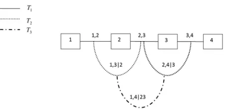
Fig. 1. A regular vine with four elements.

inference. Excellent overviews of vines are given in Refs. 16 and 17. The modeling scheme is based on a decomposition of a multivariate density into a set of bivariate copulas. The way these copulas are built up to give the overall joint distribution is determined through a structure called a vine, and can be easily visualized. A vine on n variables is a nested set of trees, where the edges of the tree j are the nodes of the tree j+1 (for j =1, . . . ,n−2), and each tree has the maximum number of edges. For example, Fig. 1 shows a vine with four variables, which con-sists of three trees (T1,T2,T3) with 3, 2, and 1 edges,

respectively. Aregular vine onnvariables is a vine in which two edges in tree jare joined by an edge in tree j+1 only if these edges share a common node, for j =1, . . . ,n−2. There aren(n−1)/2 edges in a regular vine onn variables. The formal definition is as follows.

DEFINITION 1. (Vine, regular vine)Vis a vine on

n elements if

(1) V=(T1, . . . ,Tn−1).

(2) T1 is a connected tree with nodes N1=

{1, . . . ,n}and edges E1; for i=2, . . . ,n−1, Ti

is a connected tree with nodes Ni =Ei−1.

V is a regular vine on n elements if additionally the

proximity condition holds.

(3) For i =2, . . . ,n−1, if a and b are nodes of Ti

connected by an edge in Ti, where a= {a1,a2},

b= {b1,b2}, then exactly one of the ai equals

one of the bi.

One of the simplest regular vines is shown in Fig. 1—this structure is called aD-vine; see Kurow-icka and Cooke,(14) _{p. 93. Here, T}

1 is the tree

con-sisting of the straight edges between the numbered nodes, T2 is the tree consisting of the curved edges

that join the straight edges inT1, and so on.

For a regular vine, each edge ofT1is labeled by

two numbers from{1, . . . ,n}. If we take two edges of

T1, for example, 12 and 23, which are nodes joined

by an edge inT2, then of the numbers labeling these

edges one is common to both (2), and they both have one unique number (1,3, respectively). The common number(s) will be called theconditioningset De for

that edgee(in this example, the conditioning set is simply{2}) and the other numbers will be called the

conditioned set (in this example, {1,3}). For a

reg-ular vine, the conditioned set always contains two elements.

We associate a vine distribution to a vine by spec-ifying a copula to each edge ofT1and a family of

con-ditional copulas for the concon-ditional variables given the conditioning variables, as shown by the following result of Bedford and Cooke.(15)

THEOREM 1. LetV =(T1, . . . ,Tn−1)be a regular

vine on n elements. For each edge e(j,k)∈Ti,i =

1, . . . ,n−1 with conditioned set {j,k} and

condi-tioning set De, let the conditional copula and

cop-ula density be Cj k|De and cj k|De, respectively. Let

the marginal distributions Fi with densities fi,i =

1, . . . ,n be given. Then, the vine-dependent distribu-tion is uniquely determined and has a density given by:

f(x1, . . . ,xn)= n

i=1 f(xi)

n−1

j=1

e(j,k)∈Ei

cj k|De(Fj|De(xj),Fk|De(xk)). (2)

Note that we use cj k|De here to be a

condi-tional copula density and not the more usual con-ditional bivariate cumulative distribution function (cdf) (which is not a copula). The existence of regu-lar vine distributions is discussed in detail by Bedford and Cooke.(13)

The density decomposition associated with four random variablesX=(X1, . . . ,X4) with a joint

den-sity function f(x1, . . . ,x4) satisfying a copula-vine

structure shown in Fig. 1 with the marginal densities

f1, . . . , f4is:

f1234(x1, . . . ,x4)= 4

i=1

f(xi)×c12(F(x1),F(x2))

c23(F(x2),F(x3))c34(F(x3),F(x4))×

c13|2(F(x1|x2),F(x3|x2))c24|3(F(x2|x3),

Note that in the special case of a joint normal distribution, we would use the normal copula every-where in the above expression and the conditional copulas would be constant (i.e., not depend on the conditioning variable). This means that the joint nor-mal structure is specified byn(n−1)/2 (conditional) correlation values, which are algebraically free be-tween −1 and +1 (unlike the values in a correla-tion matrix). See Bedford and Cooke(13) for more details.

Theorem 1 gives us a constructive approach to build a multivariate distribution given a vine struc-ture: if we choose marginal densities and copulas, then this will give us a multivariate density. Hence, vines can be used to model general multivariate den-sities. However, in practice we have to use copulas from a convenient class, and this class should ideally be one that allows us to approximate any copula to an arbitrary degree. In the following sections, we ad-dress this issue in more detail. By having this class of copulas, we can approximate any multivariate distri-bution using any vine structure.

Unlike the situation with Bayesian networks, where not all structures can be used to model a given distribution, the theorem shows that, in principle, any vine structure may be used to model a given distribu-tion. However, when specific families of copulas are used some vine structures work better than others. That is, given a family of copulas, some vine struc-tures give a better degree of approximation than oth-ers. We shall return to this point later.

Much work has been done to opera-tionalize the use of vines for modeling mul-tivariate data sets(11,16,18,19) _{and an R package}

“VineCopula” has been developed to imple-ment the approaches in this work (http://cran.r-project.org/web/packages/VineCopula/index.html).

It is worth stressing that the flexibility of vines gives us the potential to capture any fine-grain struc-ture within a multivariate distribution. A key as-pect that cannot be modeled by Bayesian networks is that of conditional dependence. Bayesian net-works are built around the concept of conditional

independence—arrows from a parent node to two

child nodes means that the child variables are con-ditionally, independent given the parent variable. Of course, unconditionally these two child nodes are de-pendent. However, different models of conditional dependence are not available as building blocks in Bayesian networks.

Multivariate Gaussian copulas do allow for a specification of conditional dependence, but do not

allow that dependence to change: in a multivariate normal distribution, the conditional correlation of two variables given a third may be nonzero but is al-ways constant. Our approach allows the explicit mod-eling of nonconstant conditional dependence, as we illustrate with a simple example.

The deeper a bivariate copula is in the vine hi-erarchy, the more variables will be conditioned on. If the conditional dependencies are neglected, then vines are a direct method to build flexible multivari-ate models using bivarimultivari-ate copulas as building blocks.

Acaret al.(20)argue that ignoring conditional

depen-dencies (the so-called simplifying assumption) can lead to reasonably precise approximations of the un-derlying copula (as claimed by Ref. 21), but this can in general be misleading. They develop an approach to condition parametric bivariate copulas on a single scalar variable. Stoeber et al.(22) _{repeated this}

con-cern, after studying several examples, and felt the as-sumption of an absolutely continuous vine is some-times too strong. The latter assumption is used to make the vine models tractable for inference and model selection. Lopez-Paz et al.(23) _{also reported}

that the simplifying assumption can lead to oversim-plified estimates in practice. They then extended the work of Acaret al.by developing a method for es-timation of fully conditional vines using a Gaussian Process.

2.1. Example

We consider an example involving nonconstant conditional correlations. Suppose we have three un-known quantities, X1,X2,X3, for which we wish to

specify a joint distribution. Marginally each vari-able is normally distributed, Xi ∼N(mi,si2), fori=

1,2,3, and Xi is not independent of Xj for i= j. We can represent the joint distribution between

X1,X2,X3 using a D-vine in three dimensions. That

is, specify a copula between X1,X2, one between X2,X3, and then a conditional copula between X1,X3 |X2.

In each case, we choose a bivariate Gaussian cop-ula. This takes the form, forUi =F(xi),

C(ui,uj)=ρ(−1(ui), −1(uj)),

If we were to specify a constant correlation be-tween X1,X3| X2 then the resulting distribution of X1,X2,X3could be modeled using the Gaussian

cop-ula. However, let us suppose that the correlation be-tweenX1,X3| X2is not constant but rather

ρX1,X3|X2∈(0:0.33)=1, ρX1,X3|X2∈(0.33:0.67)=0,

ρX1,X3|X2∈(0.67:1)= −1,

so that there is a positive linear relationship between the variables forU2=F2(X2) in (0,1₃), they are

un-correlatedforU2between (1₃,2₃), and there is a

nega-tive linear relationship between them in (2 3,1).

We can divide the support of X2, via U2, into

intervals. Then we can define a Gaussian copula within each interval. Suppose that numerical val-ues for the required means and standard deviations arem1=0.5,m2=1,m3= −1, ands1=s2=s3=2

and the correlations between X1,X2 and X2,X3 are ρ12 =0.75,ρ23= −0.75, respectively. This fully

spec-ifies the vine.

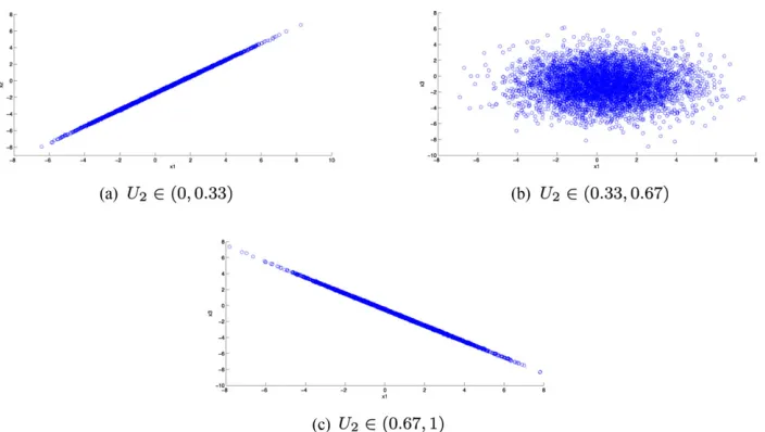
We can simulate from the vine to check that we recover the conditional correlations for X1,X3 |X2.

In order to do this, we randomly drawu1,u2,u3, three

standard uniform variables. Then

x1=F₁−1(u1),x2=F₂−_|11(u2|x1),x3=F₃−_|121(u3 |x1,x2),

where the distribution function F3|12 is found from f3|1,2(x3|x1,x2). For further details on this, see Ref.

15 and Section 5.2.1. We perform 5,000 simulations. The resultingX1,X3values are plotted in Fig. 2.

We have recovered the correlations well in each interval. The simulated correlations are ρX1,X3|U2∈(0,0.33)=0.9998, ρX1,X3|U2∈(0.33,0.67)=

−0.0032, andρX1,X3|U2∈(0.67,1)= −0.9998.

We shall use this approach when considering the example of Aas et al.(11) _{in Section 5.1. We believe}

that incorporating such nonconstant conditional cor-relations as we lay out in this article would be a use-ful addition to the R package VineCopula. By using a smooth function for the dependence instead of a piece-wise constant function as in the binning in the example above it, would be possible to apply such an approach to large, complex distributions.

The use of Gaussian copulas in financial mod-eling has come under fire for its uncritical use. Shreve(24)_{points out that the simple modeling of}

cor-relation available in the Gaussian copula does not pass validation tests, but that this did not stop its widespread adoption in the finance community.

3. BUILDING BIVARIATE MINIMUM INFORMATION COPULAS

The emphasis in this article is on approximation rather than on statistically optimal estimation tech-niques. We use minimum information methods to op-erationalize the approximation in the class of copulas used. This section discusses how the data required to specify bivariate copulas can be derived, either from expert or sampling data, and shows how this can be used to determine a minimum information copula.

We recall that when f andgare bivariate densi-ties then therelative informationof f with respect to

gis:

I(f|g)= ln(f(x,y)/g(x,y))f(x,y)dxdy.

Information is a measure of the degree of devia-tion of f from g and is minimized at 0 when f = g. Furthermore, because the information function is transformation-invariant, the relative information of

f with respect to g is the same as that between the copula for f with respect to the copula of g. This makes information a natural quantity with which to measure the degree of dependency in a copula, for if

gis an independent bivariate with the same marginal distributions as f, then I(f|g) is the same as the in-formation of the copula of f relative to the indepen-dent copula.

From the perspective of information and entropy,(25) _{a natural way to specify dependency}

constraints is through the use of moments. These can be specified either on the copula or on the underlying bivariate density (as long as we know the marginal distributions and can therefore transform from one to the other). We consider moment con-straints in which real-valued functionsh1, . . . ,hkare

required to take expected values α1, . . . , αk. By a

minimum information copula, we mean a copula that satisfies a set of constraints as above and that has minimum information (with respect to the uniform copula c(u, v)=uv) among the class of all copulas satisfying those constraints. This copula (when it exists and is unique—which is normally the case) is the “most independent” bivariate density that meets the constraints. Note that probabilities are simply expectations of identity functions and so this method of specifying constraints is not restrictive.

Fig. 2.The simulated distributions ofX1,X3givenX2in each of the intervals.

distributions. Specifically, lemma 4.4 and theorem 4.5 in Bedford and Cooke(13) _{(see also Kurowicka and}

Cooke(14)_{) show that if we take a minimal}

informa-tion copula satisfying each of the (local) constraints (on moments, rank correlation, etc.), then the result-ing joint distribution is also minimally informative given those constraints.

3.1. Data: Expert Judgment or

Random-Sample-wBased Approaches

Quantitative operations research models are typically quantified either by expert judgment or estimation from data. In our case, the minimum in-formation models are parameterized by the expected values of functionshi: [0,1]2→Rdiscussed above.

The simplest case is to consider a single function defined on the copula parameters h(u, v)=uv. Specifying the expected value of this is equivalent to specifying the Spearman rank correlation coefficient for the copula.(26) If we wanted to consider the product-moment correlation, this would entail trans-forming back to the original variables and using the function:

h(u, v)=F₁−1(u)F₂−1(v),

where F1 and F2 are the marginal distributions of

the original variables. The use of experts to specify correlations has been explored extensively in the literature (see, for example, Clemen and Reilly(7)). Hence, the methods we propose allow for common correlation-based approaches to specifying

depen-dence, as well as providing for a wider range of constraints if desired. Kurowicka et al.(27) _explored

the use of Bayesian networks to structure the specification of parameters for vine models.

We remark that the Spearman correlation can take any value between −1 and +1, whereas the product-moment correlation is typically restricted to a narrower interval depending on the marginal distri-butions involved. Bedford(28)_{discussed the}

possibili-ties of using the minimum information approach to explore the range of feasible values to aid experts in choosing consistent parameter values.

The approach taken in this context is subjec-tivist and follows a tradition in which expectation val-ues are used to specify uncertain quantities.(25,29–31)

Within a conventional Bayesian approach, our work may be thought of as a way to generate an informa-tive prior distribution. We are not suggesting that the approach be used as an alternative to Bayesian up-dating. We remark that MCMC methods have been used in conjunction with vines(16,32) in order to up-date vines.

The elicitation of a joint probability distribu-tion from experts or the approximadistribu-tion of a joint distribution of multiple uncertain quantities are among the key research areas in risk assessment, and the distinction between sources of uncertainty often comes into play in the elicitation of the un-certain quantities.(33,34)_{Uncertainties are sometimes}

method in this article can be used to approximate the joint distribution based on observed sample data for multiple uncertain quantities. Epistemic uncertainty is due to a lack of knowledge about the behavior of the system. This is conceptually resolvable.

The epistemic uncertainty can, in principle, be eliminated with sufficient study. Borgonovo(35) _and

Aven(33)_{reported that subjective probabilities are}

of-ten used for representing this type of uncertainty, but several other approaches can be used to represent this uncertainty. Therefore, our method can be used to elicit the prior distribution of unknown parame-ters by building a subjective multivariate distribution based on observable quantities. Although one may use rank correlations that are not observable quan-tities, within a minimum information framework it is possible to specify the expected value of any partic-ular function on the probability space. Rank correla-tion falls into this framework as it is linearly related to the expected value of a product of cdfs in the cop-ula space.

If we wish to fit distributions on the basis of sam-pling data (large quantities of which may be avail-able, for example, in financial risk modeling prob-lems), the data can be transformed to uniform after estimation of the marginals. This makes it possible to consider approximation, or encoding, of the data us-ing a multivariate copula, and enables us to consider ways of judging how well that approximation can be made using given families of two-dimensional copu-las. We give examples later in the article to illustrate this approach.

3.2. TheD1AD2Algorithm and Minimum

Information Copulas

Suppose there are k functions, h1,h2, . . . ,hk:

[0,1]2_{→R, for which we specify the mean values} α1, . . . , αk that these functions simultaneously take.

Further suppose thathi,hj are linearly independent

fori = j. We seek a copula that has these mean val-ues, a problem that is usually either infeasible or un-derdetermined. Assuming feasibility for the moment, we ask that the copula be minimally informative (rel-ative to the uniform distribution), which guarantees a unique and reasonable solution. Define the kernel:

A(u, v)=exp(λ1h1(u, v)+. . .+λkhk(u, v)). (4)

According to the general theory of Borweinet al.(36)

and Nussbaum(37) _{(section 4), there is a unique}

copula with minimum information satisfying the

constraints that the mean value of hi is αi (i =

1, . . . ,k), and this has density

d(1)(u)d(2)(v)A(u, v)

for some functions d(1)_{(·), d}(2)_{(·). The parameters}

(λ1, . . . , λk) depend on (α1, . . . , αk) in a

nonlin-ear way. There are numerical procedures to de-termine this relationship: given (λ1, . . . , λk) we can

numerically determine the functions d(1)_{(u) and} d(2)(v) and calculate the associated mean values for

h1,h2, . . . ,hk. By numerically solving this function, as

discussed below, we can find the unique (λ1, . . . , λk)

for which the mean values of h1,h2, . . . ,hk are α1, . . . , αk. A summary of the theory based on

Bedford and Meeuwissen,(26)_Nussbaum(37)_(section

4), and Borweinet al.(36)_{is addressed in Ref. 38.}

The general theory says that the set of all pos-sible expectation vectors (α1, . . . , αk) that could be

taken by (h1,h2, . . . ,hk) under some probability

dis-tribution is convex, and that for every (α1, . . . , αk) in

the interior of that convex set there is a density with parameters (λ1, . . . , λk) for which (h1,h2, . . . ,hk)

take these expectations.

This general approach to defining a copula was used by Bedford and Meeuwissen(26) with a single function h(u, v)=uv, which measures the Spear-man rank correlation of the copula. Bedford(28)and Lewandowski(39) have considered larger groups of functions.

The discrete version of this problem can be written in terms of matrices. In this case, the prob-ability densities defined above are approximated by probability mass functions, which are given below. Suppose that (u, v) are discretized into n

points, respectively, as ui, and vj, i,j =1, . . . ,n.

Then, we write A=(ai j),D1=diag(d₁(1),...,dn(1)), D2=diag(d1(2),...,d

(2)

n ), where ai j =A(ui, vj), di(1)= d1_(u

i), d(2)j =d2(vj). The assumption of uniform

marginals means that:

j

d_i(1)d(2)_j ai j =1/n, and

i

d_i(1)d(2)_j ai j =1/n,

∀i,j =1, . . .n.

Hence,

d_i(1)= 1

n_jd(2)_j ai j

andd(2)_j = 1 n_id_i(1)ai j

.

Finding matrices D1 and D2 so that D1AD2 is

a stochastic matrix has been long studied. Sinkhorn and Knopp(40)_{gave a simple algorithm, and the}

much used. IPF uses an iterative procedure to de-termine the entries of D1 and D2. The idea is

sim-ple: start with arbitrary positive initial matrices for

D1 and D2, then successively define new vectors by

iterating the maps:

d_i(1) → 1

n_jd(2)_j ai j

(i =1, . . . ,n),

d(2)_j → 1

n_id_i(1)ai j

, (j=1, . . . ,n).

This iteration converges geometrically to give us the vectors required. Nussbaum(37) (section 4) consid-ered the problem in greater generality, considering continuous densities and functions, and showed that the corresponding functional is a contraction map-ping on a space of functions endowed with a Hilbert projective metric. We make use of this fact when con-sidering the quality of approximations made to cop-ulas below.

To compare different discretizations (for differ-entn), we multiply each cell weightd_i(1)d(2)_j ai j byn2

as this quantity approximates the continuous copula density with respect to the uniform distribution.

As discussed above, for a given set of functions (h1, . . . ,hk), the mapping from the set of vectors of λs parameterizing the kernelAonto the expectations of the function (α1, . . . , αk) is found numerically, and

optimization techniques are used. We wish to deter-mine the appropriate set ofλs for given expectations

αi, where the expectations are calculated using the

discrete copula densityD1AD2. Define

Ll(λ1, . . . , λk) := n

i=1

n

j=1

d(1)(ui)d(2)(vj)A(ui, vj)

hl(ui, vj)−αl, l=1,2, . . . ,k. (5)

We seek the simultaneous roots of these functions and so minimize

Lsum(λ1, . . . , λk)= k

l=1

L2_l(λ1, . . . , λk).

The problem can be solved using one of Matlab’s optimization procedures, FMINSEARCH, which im-plements the Nelder-Mead simplex method.(42)_This

is used in the examples in this article.

We remark that, given the choice of func-tions (h1, . . . ,hk), we have a parametric class of

distributions with parameters the expected values (α1, . . . , αk) of (h1, . . . ,hk). However, although we

have a parametric family, we do not have a

closed-form expression for that family. Although the ker-nel in Equation (4) has a closed-form expression, the functions d(1) _{and d}(2) _{do not. They are, however,}

uniquely defined and simple to compute. Pseudo-code is given in the Supporting Information to the article.

When fitting common parametric copulas such as thet-copula using expert judgment it can be difficult to relate the parameters of the copula to observable quantities for which we can ask experts values. This is not true using minimum information copulas, how-ever, due to the flexibility of the functionshi(·). As

an example, we show how an expert could specify a copula though defining two expected values.

3.3. Example

Suppose X and Y represent the failure times of two components that are functionally identical and physically colocated. There are many reasons to believe that the distributions of Xand Ywill be dependent, but modeling all the different sources of dependency may be difficult to do explicitly. Assume that the marginal distribution functions FX and FY

are exponential with mean time to failure 100, and that we want to specify a copula for (X,Y).

We could ask an expert for information about the likelihood of near-simultaneous failure. Suppose that the expert assesses that the probability of both systems failing within time 1 of each other is 0.1, and that the probability both systems fail within time 10 of each other is 0.3. The expert information says that if we consider the functions of the copula variablesU

andV, defined by:

h1(u, v)=

1 if |F_X−1(u)−F_Y−1(v)|<1 0 otherwise, ,

h2(u, v)=

1 if |F_X−1(u)−F_Y−1(v)|<10 0 otherwise,

then the copula needs to be chosen so that the ex-pected value ofh1 is 0.1 and that ofh2is 0.3. Using

the methods discussed here we can construct the min-imum information copula.

In general, the range of expectation values avail-able to the expert will be constrained, in the first instance by the choice of marginal distribution, and then by the expected value chosen for the first func-tion. This was discussed by Bedford(28) _{in the}

for the experts, which is better than asking them to assess moments or abstract parameter values. Sec-ond, as the range of possible values for the expecta-tion of a funcexpecta-tion can be computed by evaluating the function’s expected value as we change the Lagrange multiplier values in Expression (4), we can offer guid-ance to experts about what values may be chosen to be consistent with those already chosen.

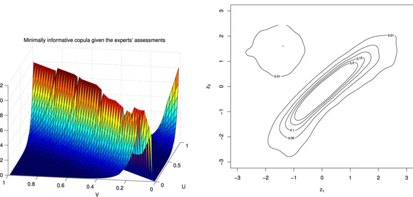
The resulting parameter values for this copula, found using a discretized grid of 200×200 points, are

λ1= −12.9100 andλ2= −1.377. The left-hand side

of Fig. 3 shows the minimally informative copula for these values.

On the right-hand side of Fig. 3, we have in-cluded a contour plot of the copula density trans-formed to allow for standard normal margins by transforming the copula coordinates (u, v) to (z1,z2)

with zj =−1(uj) for j =1,2. This allows us to

as-sess which is the closest bivariate copula to the mini-mum information copula fitted and so allows compar-ison to common parametric copulas. In the case of a Gaussian copula, the contour plots will be elliptical, while shapes like pears give indication of tail depen-dence induced, for example, by a Clayton or Gum-bel copula. Bivariatet-copulas are identified through diamond-shaped contours. In this case, we see an el-liptical shape.

4. COPULA COMPACTNESS

The previous section showed how bivariate min-imum information copulas can be constructed and provides a useful family of bivariate copulas. How-ever, the article aims to construct higher dimensional copulas. An important technical step is taken in this section where we consider the amount of variability between different bivariate copulas arising in a multi-variate copula. The key step is to show that the family of bivariate (conditional) copula densities contained in a given multivariate copula distribution forms a compact set in the space of continuous functions on [0,1]2_{. We can then show that the same finite}

param-eter family of copulas can be used to give a given level of approximation to all conditional copulas simultaneously.

It is important to define precisely the way in which we approximate densities. We assume that all densities are continuous and uniformly bounded away from zero. WriteC(Z) for the space of contin-uous real-valued functions on a space Z, where we shall always take Z=[0,1]r _{for somer. A norm on}

the spaceC(Z) is given by:

||f1...r|| =sup|f1...r(x1, . . . ,xr)|, f1...r ∈C(Z).

Since our functions are assumed continuous on Z, and since Zis compact, the norm of any such func-tion is finite. We shall be interested in the set of all possible two-dimensional (conditional) copulas asso-ciated to a given continuous density function f:

C(f)= {ci j|i1...ir : 1≤i,j,i1, . . . ,

ir ≤n,i,j =i1, . . . ,ir},

where ci j|i1...ir is the copula of the conditional den-sity of Xi,Xj given Xi1, . . . ,Xir. Thus,C(·) is an in-finite set. It will be important to show that this set is relatively compact in the space of all continuous real-valued functionsC([0,1]2_{) because then we can}

show that the copula densities can be uniformly ap-proximated. We consider compactness relative to the topology induced by the sup norm.

Compactness of a set Kcan be defined equiva-lently through one of two properties, each of which we shall use. (1) Any open cover of K has a finite subcover. In other words, ifKis a subset of an infi-nite union of open sets, then it is in fact also a subset of a finite union of those open sets. (2) Any sequence of points (which in our case are functions) ofKhas a convergent subsequence.

The Arzela-Ascoli Theorem gives another way of checking compactness when dealing with func-tion spaces. It says that a subset K⊂C([0,1]2₎

is relatively compact if the functions of K are equicontinuous and point-wise bounded. We re-call that a set of functions is equicontinuous if for all >0 and (u, v) there is a δ >0 such that if the Euclidean distance |(u, v)−(u, v)|< δ then

|g(u, v)−g(u, v)|< ∀g∈ K, and that K is point-wise bounded if sup{||g||:g∈K}<∞.

As a first step to showing the relative compact-ness ofC(f), we first consider two other spaces: the set of conditional marginal densities:

M(f)={fi|i1...ir : 1≤i,i1, . . . ,ir ≤n,i=i1, . . . ,ir},

where fi|i1...ir(xi |xi1, . . . ,xir) : [0,1]→R are the conditional densities of Xi given Xi1, . . . ,Xir, one function for each combination of conditioning val-ues xi1, . . . ,xir, and the set of conditional bivariate densities:

B(f)= {fi j|i1...ir : 1≤i,j,i1, . . . ,ir ≤n,i,

Fig. 3.A plot of the minimum information copula and transformed contour plot forX,Y.

where fi j|i1...ir is the conditional density of Xi,Xj given Xi1, . . . ,Xir. Thus, M(f),B(f) are also infi-nite sets. As we have defined it, a member ofM(f) is a function of one variable—in other words, all the different marginals that we get for different con-ditions are individually members of M(f). Simi-larly forB(f). Hence,M(f)⊂C([0,1]) andB(f)⊂

C([0,1]2).

THEOREM 2. The sets M(f)⊂C([0,1]) and

B(f)⊂C([0,1]2_{)are relatively compact.}

Proof. See Appendix A.

THEOREM 3. The setC(f)⊂C([0,1]2_{)is relatively} compact.

Proof. See Appendix A.

Since all the functions inC(f) are positive and uniformly bounded away from 0 it follows that:

COROLLARY 1. The set LN C(f)= {ln(g) :g∈

C(f)} ⊂C([0,1]2_{)is relatively compact.}

4.1. Linear Bases and Approximate Copulas

Consider the ordered set of sequences

h0,h1,h2, . . .⊂C([0,1]2). We would like any

finite sequenceh0,h1, . . . ,hnto be linearly

indepen-dent modulo the constants. The setC([0,1]2_{) can be}

considered a vector space. DefineVnto be the vector

space generated by the firstnterms in the sequence. We would also like to show that ∪nVn is dense in C([0,1]2_).

A countable basish0,h1, . . .ofC([0,1]2) over the

field R is a countable subset h0,h1, . . .⊂C([0,1]2)

with the property that every element v∈C([0,1]2₎

can be written as an infinite seriesv=∞_i=0λihi,in

exactly one way, whereλi ∈R.

Consider the countable basis h0,h1, . . .. Since v=0 can be written in exactly one way, then this must be with λi =0 for all i. This means

that any finite collection of basis elements is lin-early independent modulo the constants. If we set

h0=1, then, for any n, h1, . . . ,hn are linearly

in-dependent. It is also clear that ∪nVn is dense in C([0,1]2_{). There are lots of possible bases, for}

exam-ple,u, v,uv,u2_{, v}2_,u2_v,uv2_{, . . . .}

Given an ordered basis h1,h2, . . .∈C([0,1]2)

and a required degree of approximation >0 in the sup metric, we can consider the collection of open sets:

Uk, = {g∈C([0,1]2) : inf||g−

k

i=1

λihi||< },

where the infimum in the above definition is to be taken over all possible values of theλi. Now,Uk, is

clearly open and furthermore:

Uk, ⊂Uk+1,,

∞

k=1

Uk, =C([0,1]2).

So the Uk, form an open cover of LN C(f) and

hence by definition of compactness there is aksuch that Uk, covers LN C(f). We can state this as a

THEOREM 4. Given >0, there is a k such that any

member of LN C(f) can be approximated to within

error >0by a linear combination of h1,h2, . . . ,hk.

The same result holds forC(f) (though not nec-essarily with the samek). We call the linear combi-nationk_i=1λihian approximate copula because it is

not guaranteed to be a copula itself. The next section shows that it can be adjusted slightly to obtain a cop-ula that provides good approximation.

We remark that though we have been looking at approximation in the sense of the sup norm, one could easily look at higher order approximation. For example, if we assume that the density f1...n is

con-tinuously differentiable, then all the derivatives are continuous functions and the same arguments as used above show that they form an equicontinuous and point-wise bounded family. Following through we find that the copulas generated from f1...n are also

continuously differentiable. By using a slightly dif-ferent norm on the continuously difdif-ferentiable func-tionsC1_([0,1]2_)⊂C([0,1]2_),

||g||1= ||g|| + || d dug|| + ||

d dvg||,

we can guarantee that a similar approximation result to the above holds with point-wise approximation of the derivatives.

4.2. Ensuring that Approximating Densities are Copula Densities

Since the approximation we make of a copula density is not guaranteed to be a copula density it-self, we need to transform it to obtain a copula. This is done by weighting the density as described in Sec-tion 3.2. If we have a continuous positive real-valued function A(u, v) on [0,1]2_{, then there are}

continu-ous positive functions d(1)(u) and d(2)(v) such that

d(1)(u)d(2)(v)A(u, v) is a copula density, that is, it has uniform marginals. We call this density the C

-Projectionof Aand denote itC(A). It will be

conve-nient to denote by N(h) the normalization of a non-negative functionhwith finite integral.

We can control the error made when approxi-mating a copula by another function.

Lemma 1. Let g be a nonnegative continuous copula

density. Given >0there is aδsuch that if||g− f||< δthen||g−C(f)||< .

Proof. See Appendix A.

The reweighting functions have the same dif-ferentiability properties as the function f being reweighted. This can be seen from the integral equa-tion that they satisfy:

d(1)(u)= 1

d(2)_{(v)f(u, v)dv} and

d(2)(v)= 1

d(1)_{(u)f(u, v)du}.

We use Equation (2) to see that good approxi-mation of each conditional copula gives a good ap-proximation of the multivariate density.

5. CONSTRUCTING APPROXIMATIONS USING MINIMALLY INFORMATIVE DISTRIBUTIONS

The above discussion has shown that we can ap-proximate all conditional copulas using linear com-binations of basis functions. We did not address the question of how you choose the appropriate parameter values, and finding the parameters that would minimize the sup norm for a given copula is not an appealing procedure. An alternative that lies very close to the approach described above is to use the minimum information criterion. Given

{1,h1, . . . ,hk}: [0,1]2→Rwe seek valuesλ1, . . . , λk

so that exp(k₁λihi) is close to the copula density we

are approximating.

In the minimum information framework, we do this by fitting the moments ofhi. So if higdudv= αi then we search for the copula density with

min-imum information (with respect to the independent distribution) that has those moments. This copula density is unique and has the form:

d1(u)d2(v) exp(

i=1

=1kλihi(u, v)).

When we use a vine structure to model a mul-tivariate distribution, the vine defines a decomposi-tion of the multivariate distribudecomposi-tion into condidecomposi-tional copulas, associated to the conditioned and condition-ing sets of the vine. For example, if{i,j}is the con-ditioned set and De is the conditioning set in one

part of a vine, then the family of conditional copu-las for xi,xj given De has to be specified. Using the

minimum information approach means that we spec-ify mean values for the functionshr given the

A multivariate distribution can be approximated as follows. Specify a basis familyB(k), specify a vine structure and for each part of vine, specify either ex-pected valuesα1, . . . , αkforh1, . . . ,hkon each

pair-wise copula or functionsαm(ji| De) for the expected

values as functions of the conditioning variables, for

m=1, . . . ,k.

We remark that, since under our assumptions there is a uniform lower bound on the density of the copulas used in the representation, the uniform point-wise approximation that can be achieved im-plies information convergence in two ways. By mak-ing the copula approximations close enough, we can ensure that (i) the information of the over-all approximate multivariate copula (with respect to the independent copula) is close to that of the original multivariate copula, and (ii) the informa-tion of our approximate multivariate copula rela-tive to the original multivariate copula is close to zero.

We illustrate the procedure by applying it to two financial data sets.

5.1. Example: Stock Market Time Series

We use the same data set as considered by Aas

et al.(11)We have four time series of daily data: the

Norwegian stock index (TOTX), the MSCI world stock index, the Norwegian bond index (BRIX), and the SSBWG hedged bond index. All are for the pe-riod January 1, 1999 to July 8, 2003. We denote these four variablesT,B,M, andS.

We generate a vine approximation fitted to this data set using minimum information distribu-tions. We adopt a vine structure similar to that in Fig. 1 with variables T,B,M,S being 1,2,3,4, re-spectively. We can find the corresponding functions of the copula variables X,Y,Z, and W associated withT,M,B,S. These are defined by, for example,

hi(X,Y)=h

i(F−

1 1 (T),F−

1

2 (M)) and have the same

specified expectation, in this case E[h_i(T,M)]= E[hi(X,Y)]. The minimum information copulas

cal-culated are derived based on the copula variables

X,Y,Z,W.

Initially, we construct minimally informative copulas between each set of two adjacent vari-ables in the first tree, T1. We must decide on

which bases to take and how many discretization points to use in each case. We illustrate the recom-mended procedure for the first copula inT1, between T,M.

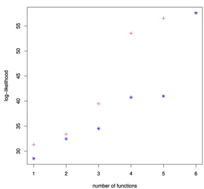
Fig. 4. The log-likelihood of the minimally informative copula cal-culated based on different functions for the simple (blue stars) and stepwise (red crosses) methods (colors visible in on-line version).

5.1.1. Step-wise Inclusion of Basis Functions

We wish to know which basis functions to in-clude in our copula. We could choose basis func-tions, starting with simple polynomials and moving to more complex ones, and include them until we are satisfied with our approximation. For example, if we included the following basis functions in or-derT M,T M2,T2M,T M3,T3M,T2M3, then the log-likelihood for the copula changes as in the blue stars in Fig. 4.

There is a jump in the log-likelihood as we add the sixth basis function, T2_M3_{. This could}

im-ply that we are not adding the basis functions in an optimal manner. Instead, at each stage, we pro-pose to assess the log-likelihood of adding each ad-ditional basis function. We include the function that produces the largest increase in the log-likelihood. Our method is similar to a step-wise regression. Do-ing so for the initial copula yields the basis func-tions T M2_,T2_M,T2_M2_{,T M,T M}4_,T2_M4_{. The}

log-likelihood at each stage is given in the red crosses in Fig. 4.

10 20 30 40 50

0

500

1000

1500

−log(error)

Number of iterations

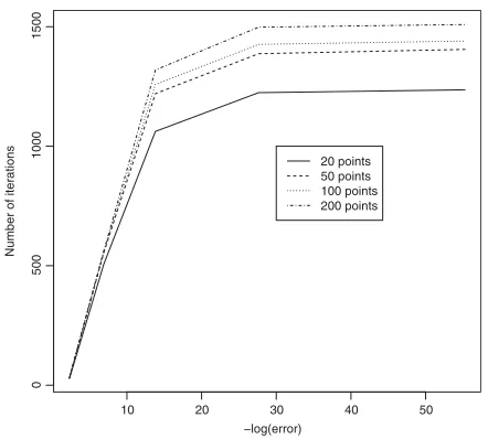
20 points 50 points 100 points 200 points

Fig. 5. A plot of the number of iterations against convergence level for 20, 50, 100, and 200 discretization points.

Jaynes(25) _{uses the parameter maximum likelihood}

estimates associated with the form of the minimum information distribution to justify the connection in the constraint rule of expectations and frequencies.

5.1.2. Returning to the Example

We include the six basis functions given above, that is, h₁(T,M)=T M2, h₂(T,M)=T2M,

h₃(T,M)=T2_M2_{, h}

4(T,M)=T M, h5(T,M)= T M4, andh₆(T,M)=T2_M4_{. We shall fix the values}

of the expectations of these functions by using the empirical data. For example, α1= _1,0941

1,094

i=1 tim2i,

as there are 1,094 observations for each variable. The minimum information copula CT M with

re-spect to the uniform distribution given the six con-straints above can be constructed. To do so, we need to decide on the number of discretization points (or grid size). A larger grid size will provide a better ap-proximation to the continuous copula but at the cost of more computation time. Similarly, the more itera-tions of the D1AD2and optimization algorithms that

are run, the more accurate the approximation will be-come. This is again at the expense of speed. Com-ments on the D1AD2 algorithm are given in Section

3.2. In terms of the optimization, we can specify how accurate we wish our approximation to be and then judge the effect on the number of iterations required for convergence. The number of iterations needed will also depend on the grid size.

Fig. 5 gives a plot comparing the number of iter-ations required for convergence of FMINSEARCH

Table I.Constraints and Parameter Values forCMBandCBS

h_i(M,B) αi λi hi(B,S) αi λi

MB 0.2905 24.970 BS 0.2375 18.818

M2B 0.2066 −22.233 B2S 0.1546 −26.914

M3_{B 0.1611 20.308 B}3_{S 0.1142 7.929}

M2_B3 _{0.1223 32.006 B}3_S2 _{0.0730 −13.949}

M2_B2 _{0.1527 −39.639 BS}2 _{0.1537 −24.939}

MB5 _{0.1142 −3.910 B}2_S2 _{0.0992 36.763}

given a certain error ofLsumand grid size. The errors

considered are in the range 1×10−1 _{to 1×10}−24_.

These are then transformed by taking −log(.) and this is the quantity plotted.

We see that the larger the number of grid points used, the larger the number of iterations needed for convergence. This is true over all error levels. The grid sizes all follow the same pattern, with large in-creases in the number of iterations needed for im-proved accuracy initially and smaller increases when the error is smaller.

Throughout the rest of the example, we choose a grid size of 200×200 and shall work to an error of 1×10−12_{. This corresponds to a transformed error}

in Fig. 5 of 27.63. This represents a suitable balance between providing an accurate approximation to the minimally informative copula and keeping computa-tional effort to a reasonable level.

We can find the minimally informative copula

CT M. Pseudo-code for doing this is given in the

Sup-porting Information. This gives parameter values of λ1=17.0262, λ2= −17.6367, λ3= −1.1117, λ4=

4.7746, λ5= −26.8054, λ6=19.9014. The copula is

plotted on the left-hand side of Fig. 6 and the con-tour plot of the copula density transformed to allow for standard normal margins is given on the right-hand side. The log-likelihood for the copula islTM=

58.1256.

The remaining copulas inT1 areCMB,CBS. The

constraint functions, constraints, and Lagrange mul-tipliers used for this copula are given in Table I. The log-likelihoods arelMB=155.18 andlBS =19.23,

re-spectively.

The conditional copulas in the second tree, T2,

can be approximated using the minimum information approach. Initially, we construct the conditional min-imum information copula betweenT| Mand B|M.

Aaset al.(11)considered the dependencies betweenT

Fig. 6.The minimally informative copula betweenTandMand transformed contour plot, Norwegian stock data.

Instead, we divide the support of Minto some arbitrary subintervals or bins and then construct the conditional copula within each bin. We will investi-gate the effect of this in the following example. We find bases in the same way as for the marginal copu-las and fit the copucopu-las to the expectations calculated for these. We use four bins so that the first copula is forT,B|M∈(0,0.25). The bases for this copula are h₁(T,B|M∈(0,0.25))=T2_B,h

2(T,B|M∈

(0,0.25))=T3_B,h

3(T,B|M∈(0,0.25))=T4B, h₄(T,B|M∈(0,0.25))=T5B,h₅(T,B|M∈

(0,0.25))=T B5_,h

6(T,B|M∈(0,0.25))=T2B4.

The expectations given these basis functions that will constrain the minimum information copula are

α1=0.1246, α2=0.0983, α3=0.0813, α4=0.0693, α5=0.0239, andα6 =0.0220.

We follow this process again for the remain-ing bins. Table II shows the constraints and corre-sponding Lagrange multipliers required to build the conditional minimum information copula between

T|M∈(0,1) and B|M∈(0,1). The overall log-likelihood of the conditional minimum information copula betweenTandBgivenM∈(0,1) is 29.242.

Similarly, we can construct the minimum infor-mation copula between M|B and S| B based on four bins and six constraints. The resulting minimum information copula has a log-likelihood of 16.3901.

The conditionally minimally informative copula in the third tree,T3, can be obtained. We first divide

each of the conditioning variables’ supports into four bins as inT2. Then, the minimum information copulas

forT|(M,B) andS|(M,B) are calculated on each

combination of bins forM,B. InT3, there are 16 bins

altogether. Details are omitted. The log-likelihood of

T3is 110.69.

The log-likelihood of the overall vine, obtained by summing the log-likelihoods of each of the com-ponent copulas, is 388.859. This is larger than that using the vine construction of bivariatet-copulas and constant conditional dependence of Aas et al.(11) of 291.801. Suppose, rather than choosing our bases using the step-wise method, we had calculated all of the copulas using the same six basis functions. Further suppose that those chosen were the simple polynomials, XY,XY2_,X2_Y,XY3_,X3_Y,X2_Y3_{. Then}

the overall log-likelihood is 370.147. This is lower than when using our approach but better than the

t-copula of Aaset al.However, the advantage of the step-wise method can be seen if we take fewer basis functions for each copula. If we take 5, we obtain a log-likelihood of 377.552, which is still larger than that obtained using 6 without the step-wise approach.

5.2. Example: Comparison with the Gaussian Copula

We consider five years of exchange rates against the U.S. dollar for four different currencies: the Great British Pound, the Euro, the Japanese Yen, and the South Korean Won. Before fitting the copula models to the data, we first remove any trends, sea-sonality, etc., from the data by fittingARMA(p,q)−

GARCH(r,s) models to each of the individual

Table II. Bases, Parameter Values, and Log-Likelihoods forCT B|M

Interval Bases Parameter Values

0<M<0.25 (T2_B,T3_B,T4_B,T5_{B,T B}5_,T2_B4_{) (26.0,−141.5,231.8,−120.0,12.4,10.6)} 0_.25_<M_<0_.5 (T B_,T B2_,T3_B,T4_B,T2_B,T2_B3_{) (−32.4,16.0,−188.2,112.2,103.3,−9.2)} 0.5<M<0.75 (T2B,T B2,T3B,T2B3,T B,T B5) (13.4,33.6,12.1,−22.2,−35.0,−4.2) 0.75<M<1 (T B2_{,T B}3_{,T B}4_{,T B,T}5_{B,T B}2_{) (−22.5,38.5,−23.6,1.7,−3.6,6.7)}

empirical cdf values of the residuals from the time-series models. For more details on this, see Ref. 11.

In order to fit a four-dimensional D-vine to the data, we need to identify a structure for the vine. Using the methods in this article, we know that we can fit any vine structure arbitrarily well using bi-variate minimum information copulas. However, we select the structure using the method given in the VineCopula package in R. This identifies the struc-ture of the vine sequentially, modeling the strongest correlations in the first tree of the vine, assuming that the bivariate copulas do not change with the condi-tioning value. Further information is given in Ref. 19. The resulting structure of the D-vine gives Euros, Great British Pounds, South Korean Won, and Japanese Yen, respectively, in the first tree. We relabel these currencies 1, 2, 3, and 4.

The Gaussian copula has been criticized for its widespread use in the financial sector in spite of evi-dence that the assumptions underlying modeling and necessary for use were not being met.(43)One such assumption of the Gaussian copula is that the condi-tional dependencies between variables in the model are constant. We apply the Gaussian copula, as well as a minimum information vine structure, to the ex-change rate data to investigate the suitability of this assumption.

The four-dimensional Gaussian copula for the currencies takes the form:

C(x1,x2,x3,x4)= −1(F1(x1)), −1(F2(x2)), −1_(F

3(x3)), −1(F4(x4))

,

where(·,·,·,·) is the cdf of the 4-variate standard Gaussian distribution with mean zero and variance matrix,−1_{(·) represents the inverse cdf of the}

uni-variate standard Gaussian distribution, andFi(·)

rep-resents the cdf for currencyi =1,2,3,4.

We first fit a Gaussian copula to the residual se-ries. The fitted values for the correlations are:

ρ12 =0.61, ρ13 =0.31, ρ14= −0.058, ρ23=0.35, ρ24 =0.027, ρ34= −0.081. (6)

Table III. The Constraints and Lagrange Multipliers for the Three Marginal Copulas in the First Tree of the Vine Copula

Variables (α1, α2, α3, α4) (λ1, λ2, λ3, λ4)

u1,u2 (0.301,0.218,0.219,0.166) (33.63,−20.15,−33.90,30.17)

u2,u3 (0.280,0.196,0.197,0.142) (26.22,−21.69,−22.49,22.21)

u3,u4 (0.244,0.162,0.159,0.105) (21.36,−25.22,−18.89,21.88)

We fit a minimum information vine and compare the two approaches by simulating from the two distributions. We fit a D-vine in four dimensions. This requires a minimum information copula spec-ified between exchange rates 1 and 2, one between 2 and 3, and another between rates 3 and 4, a conditional copula between rates 1 and 3 given exchange rate 2 and between rates 2 and 4 given exchange rate 3, and a conditional copula between rates 1 and 4 given exchange rates 2 and 3. We specify four basis functions for each copula and use the same basis functions each time, namely,

h1(ui,uj)=uiuj,h2(ui,uj)=u2iuj,h3(ui,uj)= uiu2j,h4(ui,uj)=ui2u2j for i =1,2,3,j=i. We

could have used the method from the previous example to choose the optimal basis functions.

Table III gives a summary of the constraints and resulting parameter values for the marginal copu-las. The copulas are given in the top three plots of Fig. 7 and the contour plot of the copula density transformed to allow for standard normal margins are given, respectively, at the bottom of the figure.

We wish to split the support ofu2 into bins and

define the conditional copula foru1 andu3based on

these bins. After plotting the conditional correlations for several different numbers of bins, we settle on four bins.

The remaining copula is that betweenu1 andu4.

To construct this, we must create bins of combina-tions ofu2 and u3. We separateu2 andu3 into four

Fig. 7. The bivariate minimum information copulas (top) and transformed contour plots (bottom) for the exchange rates of currencies 1 and 2, 2 and 3, and 3 and 4, respectively.

0.1 0.2

0.3 0.4

0.5 0.6

0.7 0.8

0.9

0.1 0.2 0.3 0.4 0.5 0.6 0.7 0.8 0.9 −0. 4 −0.3 −0.2 −0.1 0 0.1 0.2 0.3

Fig. 8.The changes in conditional correlation between exchange rates 1 and 4 given different bins for exchange rates 2 and 3.

u1 andu4 for each of these bins and plot them as a

surface, as in Fig. 8.

The empirical conditional expectation data are not inconsistent with the conditional correlation be-ing a smooth function. The use of a smooth curve

to represent the conditional correlation is a possible way of compressing the data more compactly.