Title Distorted mix method for constructing copulas with taildependence
Author(s) Li, L; Yuen, KC; Yang, J
Citation Insurance: Mathematics and Economics, 2014, v. 57, p. 77-89
Issued Date 2014
URL http://hdl.handle.net/10722/199239
Rights
NOTICE: this is the author’s version of a work that was accepted for publication in Insurance: Mathematics and Economics.
Changes resulting from the publishing process, such as peer review, editing, corrections, structural formatting, and other quality control mechanisms may not be reflected in this
document. Changes may have been made to this work since it was submitted for publication. A definitive version was
subsequently published in Insurance: Mathematics and Economics, 2014, v. 57, p. 77-89. DOI:
Distorted Mix Method for Constructing Copulas with
Tail Dependence
Lujun Li
∗K. C. Yuen
†Jingping Yang
‡April 2014
Abstract
This paper introduces a method for constructing copula functions by combining the ideas of distortion and convex sum, named Distorted Mix Method. The method mixes different copulas with distorted margins to construct new copula functions, and it enables us to model the dependence structure of risks by handling central and tail parts separately. By applying the method we can modify the tail dependence of a given copula to any desired level measured by tail dependence function and tail dependence coefficients of marginal distributions. As an application, a tight bound for asymptotic Value-at-Risk of order statistics is obtained by using the method. An empirical study shows that copulas constructed by this method fit the empirical data of SPX 500 Index and FTSE 100 Index very well in both central and tail parts.
Keywords: copula; Distorted Mix Method; distortion function; tail dependence coefficient; tail dependence function.
1
Introduction
Copula method can be applied for describing the full dependence structure of random vectors. Essentially, a copula function is a joint distribution with all uniform[0,1]margins. It is known that the copula function provides a complete description of dependence structure among random vari-ables by uniting marginal distributions via Sklar Theorem. LetF(x1, . . . ,xd)be a d-dimensional
joint distribution with marginal distributions F1(x1), . . . ,Fd(xd). Sklar Theorem states that there exists a copula functionCsatisfying
F(x1, . . . ,xd) =C(F1(x1), . . . ,Fd(xd)).
∗Department of Financial Mathematics, Peking University, Beijing 100871, China. Email address: [email protected]
†Department of Statistics and Actuarial Science, The University of Hong Kong, Pokfulam Road, Hong Kong.
Email address: [email protected]
‡LMEQF, Department of Financial Mathematics, Peking University, Beijing 100871, China. Email address:
See Joe (1997) and Nelsen (2006) for more introduction about copula functions. In fact, now copula method becomes more and more important in quantitative finance and risk management, seeMcNeil et al.(2005) andDenuit et al.(2005).
Gaussian copula and Archimedean copula are important copula families applied in finance and insurance. Proposed by Li (2000), Gaussian copula has been widely used in credit risk model-ing, and it is also criticized after the subprime mortgage crisis for its incapacity to capture high correlation in tails (Donnelly and Embrechts, 2010). As an alternative for Gaussian copula, Stu-dent T-copula is capable of capturing high correlation in tails, but unfortunately StuStu-dent T-copula can not describe the asymmetry between the lower and upper tails. In high-dimensional case, Archimedean copula is very popular for its explicit expression and its convenience for sampling. However, most of the Archimedean families have few parameters, which makes the copulas ex-changeable and less flexible. Therefore, it will be important to construct copula functions sharing the good properties of several copula families.
Fundamental transformation-based copula construction methods include convex sum, ordinal sum and shuffle of copula (Nelsen, 2006). Recently, the distortion function has been applied for constructing copula functions. A continuous functionD(x)from[0,1]to[0,1]is called a distortion function if D is increasing and D(0) = 0,D(1) = 1. Yaari (1987) firstly applied the distortion function in dual theory of choice under risk, andWang(1996) defined Wang’s premium principle by using distortion functions.Genest and Rivest(2001),Klement et al.(2005),Durante and Sempi
(2005) and Durante et al. (2010) considered transformations from a bivariate copula C(u1,u2) to another one Cϕ = ϕ−1(C(ϕ(u1),ϕ(u2))), where ϕ is a distortion function. Morillas (2005) extended this idea to multivariate copulas. In addition, Liebscher (2008) presented two general construction schemes based on product of copulas and generalized Archimedean family. Fischer and Köck(2012) unified the above transformation-based methods.
In this paper, we will introduce a method called Distorted Mix Method (DMM) to construct copulas by applying distortion functions. The idea of DMM is based on the convex sum method, while the copula margins are modified by some distortion functions. By applying the distortion functions, we can model dependence structure by handling central and tail parts separately. More precisely, DMM enables us to modify the tail parts of a given copula to any desired pattern. Our theoretical discussion will focus on two tail dependence measures: tail dependence coefficients of marginal distributions and tail dependence function defined inKlüppelberg et al.(2008) andJoe et al.(2010). Through choosing suitable distortion functions, DMM can be applied to construct cop-ulas being close to a given copula, and its tail dependence can reach any desired level. Empirical results will also be given to show that a modified Gaussian copula constructed by DMM performs significantly better than Gaussian copulas in the tail parts.
This paper is organized as follows. In Section 2, we introduce our definition of DMM, and theoretical results about tail behavior of the constructed copulas are provided. In Section 3, we apply DMM to change tail dependence of a given copula, in which we focus on two tail measures: tail dependence function and tail dependence coefficients of marginal distributions. Empirical results are presented in Section 4 and conclusion is given in Section 5. Some proofs are provided in the appendix.
2
Distorted Mix Method
2.1
Definition for Distorted Mix Method
Given integerm≥2 and the corresponding weightsαi>0,i=1,2, . . . ,mwith∑mi=1αi=1, let
the distortion functionsDi j,i=1, . . . ,m, j=1, . . . ,dsatisfy the following assumption:
• Assumption A:∑mi=1αiDi j(x) =xfor any j=1, . . . ,d.
Then based on copula functionsCi,i=1, . . . ,mand the distortion functionsDi j,i=1, . . . ,m, j= 1, . . . ,d, we define a function ˜C(u1, . . . ,ud)as ˜ C(u1, . . . ,ud) = m
∑
i=1 αi·Ci(Di1(u1), . . . ,Did(ud)). (1)The above definition combines the ideas of distortion and convex sum, so we name this method Distorted Mix Method (DMM).
Next theorem will show that the function ˜C(u1, . . . ,ud)is a copula function underAssumption A, regardless of the choice of copulas, distortion functions and corresponding weights. The proof will be given in the appendix.
Theorem 1. Assume thatAssumption Aholds. Then the functionC˜(u1, . . . ,ud)defined in(1)is a copula function. Moreover, for i=1, . . . ,m,
sup (u1,...,ud)∈[0,1]d C˜(u1, . . . ,ud)−Ci(u1, . . . ,ud) ≤min{1,(1−αi)(d+1)} (2) and ˆ [0,1]d C˜(u1, . . . ,ud)−Ci(u1, . . . ,ud) du1. . .dud≤min{1,(1−αi)(d/2+1)}. (3) In the next we call the copula ˜C a DM copula, and we call copulasCi,i=1, . . . ,m the com-ponent copulas. Essentially, a DM copula is a mixture of different comcom-ponent copulas with mar-gins modified by some distortion functions. Notice that for each fixed i, the choice of the com-ponent copulaCi is irrelevant to the choice of weight αi and corresponding distortion functions Di j, j=1, . . . ,d.
Intuitively, as the weight αi gets larger, the DM copula ˜C will get closer to the component
copulaCi. The above inequalities (2) and (3) show that the DM copula ˜Cis close toCiwhenαiis
close to 1.
We can explain DM copula from the following two viewpoints. The first is that DMM is a generalization of the convex sum method. LettingDi j(u) =u, ˜C(u1, . . . ,ud)can be expressed as a convex sum ˜ C(u1, . . . ,ud) = m
∑
i=1 αi·Ci(u1, . . . ,ud).Compared with the convex sum method, DMM uses a technique of distortion to make each com-ponent copula focus on a particular aspect. The second viewpoint is that DM copula can be derived
from convex sum of distribution functions. LetHandHibed-dimensional continuous distributions satisfying H(x1, . . . ,xd) = m
∑
i=1 αi·Hi(x1, . . . ,xd).Note thatHandHican also be expressed as
H(x1, . . . ,xd) =C(F1(x1), . . . ,Fd(xd)), Hi(x1, . . . ,xd) =Ci(Fi1(x1), . . . ,Fid(xd)),
whereC,Ci are copula functions, and Fi,Fi j are marginal distributions. Then the above copula functionCcan be written as
C(u1, . . . ,ud) = m
∑
i=1 αi·Ci Fi1 F1−1(u1) , . . . ,Fid Fd−1(ud),which shows that the distortion function Di j can be regarded as a transformation between the margins
Di j(x) =Fi j
Fj−1(x).
In the next, we provide a factor illustration to explain DMM from the view of random variables. Based on this view, we can get a better understanding of DM copula and its distortion functions.
Proposition 1. Consider a common factor Z distributing discretely as P(Z = i) = αi for i =
1, . . . ,m. For each fixed i, the random variables U1, . . . ,Ud satisfy thatP(Uj≤x|Z=i) =Di j(x), and their conditional copula under Z = i is denoted as Ci(u1, . . . ,ud). Then if Assumption A
holds, the joint distribution of U1, . . . ,Ud is the DM copula defined in(1).
The proof of the proposition is obvious and omitted. The above proposition provides a clear probability structure for DM copulas. It shows that DM copulas can describe different dependence structures in different market circumstances, which is quite reasonable in finance (Longin and Solnik,2001).
Owing to the factor illustration of DM copulas, the procedure of sampling a DM copula can be divided into two parts: first sample each component copulaCi, then compute the inverse functions
D−i j1. More precisely, to sample a random vector U= (U1, . . . ,Ud)whose joint distribution is ˜C
defined in equation (1), we can work on it according to the following steps:
1. Sample a random variable Z distributing discretely asP(Z=i) =αifor i=1, . . . ,m;
2. Sample a random vectorV= (V1, . . . ,Vd)whose joint distribution function is CZ;
3. Let Uj=D−Z j1(Vj).
ThenU= (U1, . . . ,Ud)is a sample of ˜C. This algorithm provides a sampling scheme based on each
component copula, which avoids sampling directly based on the expression of ˜C. Therefore, if all the component copulas are easy to sample, it will also be easy to sample the DM copula.
Besides the advantage in simulation, the DM copula inherits many good properties from its component copulas. For instance, if all the component copulasCiand the distortion functionsDi j
have continuous density functions, then the DM copula also has a continuous density function. In most cases of the following discussion, we assume that the distortion functions in the same component copula are identical. Precisely, let Di:=Di1=Di2 =. . .=Did for eachi, then As-sumption Ais simplified as
• Assumption B:∑mi=1αiDi(x) =x.
UnderAssumption B, the DM copula is simplified as
˜ C(u1, . . . ,ud) = m
∑
i=1 αi·Ci(Di(u1), . . . ,Di(ud)). (4) Remark1. If the distortion functions in the same vector component are identical, i.e.,D1j=D2j=. . .=Dm j for all j, thenAssumption Aimplies that all the distortion functions are simply reduced toDi j(x) =x. In this case, the DM copula becomes the convex sum of the component copulas.
2.2
Examples of DM copulas
As is well known, Gaussian copula can not describe heavy tail correlation of financial variables. Next we construct a more flexible copula family by using DMM. The intuitive idea is to modify a Gaussian copula into a new copula with Archimedean tails.
Example 1. LetC1 be a d-dimensional Gaussian copulaCN
Σ with correlation matrixΣ, C2 be a
Clayton copulaCCl
θ andC3be a Gumbel copulaC Gu ψ , i.e., CθCl(u1, . . . ,ud) = d
∑
j=1 u−θ j −d+1 !−1θ , CψGu(u1, . . . ,ud) =exp − " d∑
j=1 −lnujψ #ψ1 and CΣN(u1, . . . ,ud) =ΦΣ Φ−1(u1), . . . ,Φ−1(ud) ,where θ ∈(0,∞), ψ ∈[1,∞), Φ is the univariate Gaussian distribution function and ΦΣ is the
multivariate Gaussian distribution function with correlation matrixΣ.
Letα ∈(0,12),α1=1−2α,α2=α3=α, and choose the distortion functions
D2(x) = x−αx 2 α+ (1−2α)x,D3(x) = αx2 α+ (1−2α)(1−x),D1(x) = x−αD2(x)−αD3(x) 1−2α . (5)
It is easy to check∑3i=1αiDi(x) =x, soAssumption Bholds. According to Theorem 1, the DM
copula defined in (4) is close to the Gaussian copulaCN
Σ whenα is small. Furthermore, the
numer-ical results in Figure2show that the DM copula performs like a Clayton copula in the lower tail, and like a Gumbel copula in the upper tail. Here we only provide an intuitive explanation, and the theoretical results will be given in the next subsection.
For the above DM copula, we consider its factor illustration in Proposition 1. Suppose there is a common factor Z taking values in {1,2,3}. According to Proposition1, let (U1, . . . ,Ud) be a sample of the DM copula, then the conditional distribution functions ofUj, j=1, . . . ,d under
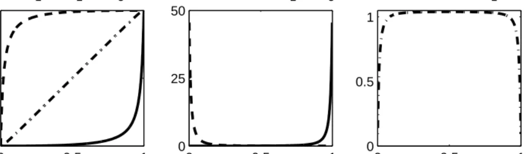
Z = i are all equal to Di(x). Figure 1 shows the conditional distribution functions D1,D2,D3 and their density functions D01,D02,D03 when α =0.02. The density functions D02,D03 imply that
Uj, j=1, . . . ,dare more likely to take small values underZ=2 and take large values underZ=3. On the other hand, Proposition1says that the conditional copula ofU1, . . . ,Ud underZ=2 is the
0 0.5 1 0 0.5 1 (a) D 1(x), D2(x), D3(x) 0 0.5 1 0 25 50 (b) Densities of D 2(x),D3(x) 0 0.5 1 0 0.5 1 (c) Density of D 1(x)
Figure 1: Subplot (a) shows the distortion functionsD1(x),D2(x),D3(x)defined in (5) when α =0.02.
Subplot (b) and (c) show the density functionsD01,D02,D03whenα=0.02. The dash dotted, dashed and solid
lines areD1,D2,D3and their density functions respectively.
Clayton copulaCCl
θ , so the lower tail of the DM copula performs like a Clayton copula. Similarly,
the upper tail of the DM copula performs like a Gumbel copula.
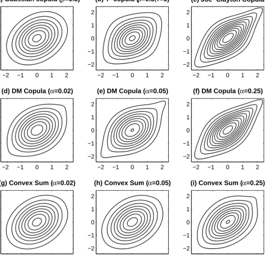
Figure2shows density contours of bivariate meta-distributions with different bivariate copulas and standard Gaussian margins. The DM copulas in Figure2(d)-Figure2(f)are defined in Example
1. Here the component Gaussian copulaCρNhas correlationρ=0.3, the component Clayton copula
CCl
θ hasθ =0.7565, and the component Gumbel copulaC Gu
ψ hasψ =1.7095. Figure2(g)-Figure 2(i)display the cases of convex sum copula
CCs(u1,u2) = (1−2α)·CNρ(u1,u2) +α·CClθ (u1,u2) +α·CGuψ (u1,u2). (6) Joe-Clayton copula in Figure2(c)is defined inJoe(1997) as
CJc(u,v) =1− 1−h(1−(1−u)ψ)−θ + (1−(1−v)ψ)−θ− 1i−1/θ 1/ψ , (7)
in which(θ,ψ)∈(0,∞)×[1,∞). Here we chooseθ =0.7565 andψ =1.7095 as above.
Compared with the convex sum copulas, the DM copulas show greater flexibility. Whenα =
0.02 in Figure2(d), the weightα1of the component Gaussian copula is 0.96. Sinceα1is close to 1, the DM copula is similar to the Gaussian copula, hence the contours in Figure2(d)look like the Gaussian density contours in Figure2(a). However, the DM copula performs like a Clayton copula in the lower tail and like a Gumbel copula in the upper tail, so the tail contours are sharper than those of Gaussian density. Asα increases, the weight of component Gaussian copula decreases,
and the density contours turn to be spindle-shaped. It is interesting that the density contours with
α =0.25 in Figure2(f)are remarkably similar to those of the Joe-Clayton copula in Figure2(c).
In summary, this example shows roughly that DMM enables us to construct copulas by choos-ing central and tail parts separately.
2.3
Tail dependence modification
Tail dependence coefficient (TDC) is the most popular measure of tail correlation. For a
(a) Gaussian copula (ρ=0.3) −2 −1 0 1 2 −2 −1 0 1 2 (b) T−copula (ρ=0.3,ν=5) −2 −1 0 1 2 −2 −1 0 1 2 (c) Joe−Clayton Copula −2 −1 0 1 2 −2 −1 0 1 2 (d) DM Copula (α=0.02) −2 −1 0 1 2 −2 −1 0 1 2 (e) DM Copula (α=0.05) −2 −1 0 1 2 −2 −1 0 1 2 (f) DM Copula (α=0.25) −2 −1 0 1 2 −2 −1 0 1 2 (g) Convex Sum (α=0.02) −2 −1 0 1 2 −2 −1 0 1 2 (h) Convex Sum (α=0.05) −2 −1 0 1 2 −2 −1 0 1 2
(i) Convex Sum (α=0.25)
−2 −1 0 1 2 −2 −1 0 1 2
Figure 2: Density contours of meta-distributions with nine different bivariate copulas and standard Gaus-sian margins. DM copulas are mixed by distorted GausGaus-sian, Clayton and Gumbel copula with differentαin Example1.
limit exists. And the upper TDC is defined as the lower TDC of its survival copula, i.e., λC∗=
limu↓0Cˆ(u, . . . ,u)/u. Here the survival copula ˆCof copula functionCis defined as ˆ
C(u1,u2, . . . ,ud) =P(U1≥1−u1, . . . ,Ud≥1−ud),
whereU= (U1, . . . ,Ud)is a sample ofC. Both the lower TDC and the upper TDC are in[0,1], and large TDC corresponds to strong correlation in tail parts.
The concept of TDC can be extended to the concept of tail dependence function (TDF) de-fined byKlüppelberg et al.(2008). Its copula version has been introduced byJoe et al.(2010) as following. The lower TDF is defined as
b(w1, . . . ,wd;C) =lim
u↓0C(w1u, . . . ,wdu))/u, and the upper TDF is defined as
b∗(w1, . . . ,wd;C) =lim
u↓0 ˆ
in which(w1, . . . ,wd)∈[0,∞)d. Notice thatb(1, . . . ,1;C) =λC andb∗(1, . . . ,1;C) =λC∗. Unless
specially stated, we assume TDC and TDF always exist afterwards.
Next we extend Example 1 to a more general case. Our purpose is to replace the TDF of a given copula, sayC1. Assuming that we have a copulaC2at hand, we prefer the TDF ofC2to that ofC1. For this purpose we will construct a copula function ˜Cclose toC1 and its TDF is identical to that ofC2.
Proposition 2. Assume that C1,C2are copulas andα1,α2,D1,D2satisfyAssumption B, then the
distance between the DM copula
˜
C(u1, . . . ,ud) =α1C1(D1(u1), . . . ,D1(ud)) +α2C2(D2(u1), . . . ,D2(ud)) and C1can be measured by(2)and(3)for i=1. Furthermore,
(I) ifα2D02(0+) =1, the DM copulaC and copula C˜ 2have identical lower TDF;
(II) ifα2D02(1−) =1, the DM copulaC and copula C˜ 2have identical upper TDF.
Proof. Here we only prove the lower tail case in part (I), and the proof of the part (II) is similar. For thed-dimensional copulasCi, ifD0i(0+)exists,
lim u↓0 Ci(w1Di(u), . . . ,wdDi(u)) u =limu↓0 Ci(w1Di(u), . . . ,wdDi(u)) Di(u) · Di(u) u =D0i(0+)·b(w1, . . . ,wd;Ci).
Owing to the Lipchitz property of copula function, for a smalluwe have
|Ci(w1Di(u), . . . ,wdDi(u))−Ci(Di(w1u), . . . ,Di(wdu))| ≤ d
∑
j=1 wjDi(u)−Di(wju) =o(u). By integrating the above two aspects, we havelim u↓0 Ci(Di(w1u), . . . ,Di(wdu)) u =D 0 i(0+)·b(w1, . . . ,wd;Ci), ∀(w1, . . . ,wd)∈[0,∞)d. (8)
Now we go back to the proof of Proposition 2. Fromα1D1(x) +α2D2(x) =xwe know that
α1D01(0+) =0. Applying (8), we have
b(w1, . . . ,wd; ˜C) =α1D01(0+)·b(w1, . . . ,wd;C1) +α2D02(0+)·b(w1, . . . ,wd;C2) =b(w1, . . . ,wd;C2)
for any(w1, . . . ,wd)∈[0,∞)d.
Another idea is using other two different copulas to replace the lower and upper TDF respec-tively, which makes the lower and upper TDF belong to different types.
Proposition 3. Assume Ci,i=1,2,3are copulas andαi,Di,i=1,2,3satisfyAssumption B, then the distance between the DM copula
˜ C(u1, . . . ,ud) = 3
∑
i=1 αiCi(Di(u1), . . . ,Di(ud)) (9) and C1can be measured by(2)and(3)for i=1. Furthermore, ifα2D02(0+) =α3D03(1−) =1, theThe proof is similar and omitted. Next we provide three distortion function families Hαp(x) =x1/α, He α(x) =x 2e(1/α−2)(x−1) , Hf α,β(x) = α βx2 α β+ (1−2α) 1−xβ, (10)
where α,β >0. These distortion functions all have continuous derivatives on [0,1], and each
of them satisfies H0(1) =1/α and H0(0) =0. Notice that if H(x) is a distortion function, then
G(x) =1−H(1−x)is also a distortion function satisfyingG0(1) =H0(0)andG0(0) =H0(1). Thus if we chooseD2(x) =1−(1−x)1/α2 for example, thenα
2D02(0+) =1. The above candidates of distortion functions satisfy the conditions in Proposition2and Proposition3.
Example1(continued). The distortion function in Example1is the case 1−D2(1−x) =D3(x) =
Hf
α,1(x), so the DM copulas ˜C in Example 1 have identical lower TDF with Clayton copula and
identical upper TDF with Gumbel copula. Hence its lower and upper TDC satisfies
λC˜,λC∗˜=
2−1/θ,2−21/ψ, (
θ,ψ)∈(0,∞)×[1,∞),
which implies(λC˜,λ∗˜
C)can vary freely in(0,1)
2. Thus all the DM copulas in Figure2(d)-Figure
2(f)have the same lower TDC 2−1/0.7565=0.4 and the same upper TDC 2−21/1.7095=0.5.
Remark 2. From the discussion above, we can confirm the advantage of DMM over the convex sum method. Although convex sum is widely used as a tool in time series empirical study (Chen and Fan,2006), the convex sum copula is incapable of letting its lower and upper TDC vary freely in[0,1]2. More precisely, for the convex sum copulaCCsdefined in equation (6),we haveλCCs≤α2
andλC∗Cs ≤α3, thusλCCs+λ∗
CCs≤1 follows.
2.4
On
α
i’s selection
In this subsection, we discuss on how to select the weightsα1, . . . ,αm. For simplicity, we will
focus on the DM copula defined in the following form ˜ C(u1, . . . ,ud) = 3
∑
i=1 αiCi(Di(u1), . . . ,Di(ud)), (11)where the component copulaC1is intentionally chosen to capture the central part, and the copulas
C2andC3 are chosen to capture the lower tail part and the upper tail part separately. In practice, the copulaC1may belong to some commonly used copula family with improper tails, for example Gaussian copulas, andC2,C3 belong to some copula families whose lower/upper TDC can vary freely in[0,1]. As mentioned in Proposition3, the DM copula in (11) can be applied to modify the tail parts of copulaC1into the patterns ofC2andC3.
By the definition of DM copula, the distortion functions D1(u),D2(u),D3(u)and the weights
α1,α2,α3≥0 withα1+α2+α3=1 must satisfy the following condition
α1D1(u) +α2D2(u) +α3D3(u) =u, ∀u∈[0,1] (12) On the other hand, the condition
is required to guarantee that the DM copula ˜Chas identical lower TDF withC2and identical upper TDF withC3. Under the constraints of (12) and (13), the distortion functionsD1(u),D2(u),D3(u) are related to the parameters α1,α2 and α3. The distortion functions can be chosen from some parametric families. Some distortion functions belonging to the power, exponential and fractional families are provided in (10), in which the distortion functions are fully or partially determined by the weight parameters. More generally, we can get other parametric distortion families by the following method:
• Choose two parametric positive continuous functions h2,h3 with domain [0,1] satisfying
h2(x) +h3(x)≤1,x∈[0,1]and h2(0) =1,h2(1) =0, ˆ 1 0 h2(x)dx=α2, h3(0) =0,h3(1) =1, ˆ 1 0 h3(x)dx=α3; • Set D2(u) = ˆ u 0 h2(x) α2 dx, D3(u) = ˆ u 0 h3(x) α3 dx, D1(u) = ˆ u 0 1−h2(x)−h3(x) 1−α2−α3 dx, thenD1(u),D2(u),D3(u)are distortion functions satisfying (12) and (13).
In the next, we discuss on how to estimate the parametersα1,α2andα3.
For the purpose of our DM method, ˜C should be close to copula C1 and have the same tail patterns asC2andC3. Note that when (13) holds, the lower and upper TDFs of the DM copula ˜C are fully determined by the component copulasC2,C3and independent to the values of the weights
α1,α2,α3. On the other hand, the difference between the DM copula ˜Cand its component copula
C1is highly related to the value of 1−α1. Precisely, from (2) we see that
sup (u1,...,ud)∈[0,1]d C˜(u1, . . . ,ud)−C1(u1, . . . ,ud) ≤(1−α1)(d+1).
Thus in order that ˜C andC1 are close enough, one requirement is that 1−α1=α2+α3 is small. Therefore, we can consider estimatingα2,α3 in a small range, say[0,β]. Thus, with given
para-metric distortion functions D1,D2 and D3 satisfying (12) and (13), statistical estimation can be applied to estimateα2,α3∈[0,β]and other parameters.
The estimation of the DM copula can be implemented by the following procedure:
• Step 1: Use a parametric copula family to fit the data and estimate the parameters. DenoteC1
as the fitted copula. If the copulaC1doesn’t fit the tail parts very well, we do the following steps to modifyC1by DMM.
• Step 2: Choose the families of the component copulasC2,C3 and the distortion functions
D1,D2andD3to model the tail parts. Note thatα1+α2+α3=1, and the distortion functions are also related toα2andα3.One can set the weightsα2andα3as constants, or limitα2,α3 in a pre-set range.
• Step 3: Calibrate the parameters inC2,C3,D1,D2 andD3 by Maximum Likelihood Estima-tion (MLE). If the parametersα2,α3are unknown before this step, then the estimates of the two parameters can be obtained in this step.
In Section 4, we will apply the above procedure to analyze financial return data.
3
Constructing copulas with tail dependence by DMM
In this section, we will discuss on modifying a given copula to meet some specific tail require-ments by applying DMM. Here we consider two tail measures: tail dependence function (TDF) and tail dependence coefficients (TDC) of marginal distributions. We will only focus on the lower tail in this section, and the results of upper tail are similar.
3.1
Constructing Copulas with preferred TDF
In Section 2.3, we used DMM to replace the TDF of a given copula. Of course doing such a procedure has a certain premise that we have already chosen the alternative copula. If there is no candidate, we can focus on TDF directly. In the following, we will discuss on constructing copula functions with the objective TDF by DMM.
Joe et al.(2010) has discussed the properties of a TDF. They proved that a TDFb(w1, . . . ,wd;C) must be a groundedd-increasing function with homogeneity of order 1. Precisely,
1. (grounded)b(w1, . . . ,wd;C) =0 if there exists somewi=0; 2. (d-increasing)∑2i1=1. . .∑2id=1(−1) i1+...+idb(w(i1) 1 , . . . ,w (id) d ;C)≥0 forw (1) i ≤w (2) i ,i=1, . . . ,d;
3. (homogeneity of order 1)b(λw1, . . . ,λwd;C) =λ·b(w1, . . . ,wd;C)for anyλ ≥0.
Next we will give the necessary and sufficient conditions for a function being a TDF, then we will construct copulas with any given TDF by DMM.
Theorem 2. (I) Function B is a TDF, i.e., there exists a d-dimensional copula whose TDF equals B, if and only if B satisfies all the following conditions:
(a) B is a grounded and d-increasing function with homogeneity of order 1.
(b) B is Lipschitz continuous with parameter 1, i.e.,|B(w1, . . . ,wd)−B(v1, . . . ,vd)| ≤∑di=1|wi−vi|. (II) Assume that function B is a TDF. For(u1, . . . ,ud)∈[0,1]d, we denote
CB(u1, . . . ,ud) = B(u1, . . . ,ud), if B(1, . . . ,1) =1; B(u1, . . . ,ud) + ∏ d i=1(ui−Bi(ui)) (1−B(1,...,1))d−1, otherwise, (14)
where Bi(x) = B(x1, . . . ,xd)|xi=x&xj=1,∀j6=i, then C
B(u
1, . . . ,ud)in[0,1]d is a copula function. And for any given copula C1, the TDF of the DM copula
˜
C(u1,u2, . . . ,ud) = (1−α)C1(D1(u1), . . . ,D1(ud)) +αCB(D2(u1), . . . ,D2(ud)) (15) equals B when distortion functions D1,D2 satisfy (1−α)D1(x) +αD2(x) =x for x∈[0,1] and
αD02(0+) =1. Furthermore, the distance between the DM copulaC and copula C˜ 1 can be
Proof. The necessity of property (a) has been proved inJoe et al.(2010). The necessity of Lipschitz property in (b) is inherited from the Lipschitz property of copula function. Next we prove the sufficiency of these properties by constructing copulas with such TDF.
IfBis a function satisfying the conditions in (a) and (b), we prove thatCBis a copula function. Firstly, we notice thatBsatisfies the Lipschitz property in (b), which impliesBi(x)−Bi(0)≤x−0.
HenceBi(x)≤xfor anyi=1, . . . ,d, so we obtainB(1, . . . ,1) =B1(1)≤1.
Case 1: B(1, . . . ,1) =1. Then Bi(1) =1 for i=1, . . . ,d. The Lipschitz property implies
Bi(1)−Bi(x)≤1−xfor x∈[0,1], so Bi(x)≥x,x∈[0,1]. On the other hand, we have already
provedBi(x)≤x, soBi(x) =xforx∈[0,1]andi=1, . . . ,d. Therefore,Bhas uniform margins in [0,1]. Combining with the assumption thatBisd-increasing, we knowB(u1, . . . ,ud),(u1, . . . ,ud)∈
[0,1]dis a copula function.
Case 2: B(1, . . . ,1)6=1. Then B(1, . . . ,1)<1. Owing to the Lipschitz property, for any 0≤ x≤y ≤1 and i =1, . . . ,d, we know Bi(y)−Bi(x) ≤y−x, so x−Bi(x) is increasing for
i=1, . . . ,d. Hence∏di=1(ui−Bi(ui)) isd-increasing. Combining with the assumption thatB is
d-increasing, we knowCB is also d-increasing from (14). And it is easy to verify thatCB has uniform [0,1] margins, soCB is indeed a copula function.
Next we prove that the TDF of copulaCBequalsB. The caseB(1, . . . ,1) =1 is obvious. When
B(1, . . . ,1)<1, we compute directly based on (14),
B(w1, . . . ,wd)≤b(w1, . . . ,wd;CB)≤B(w1, . . . ,wd) +lim
u↓0 u
d−1=B(w
1, . . . ,wd),
sob(w1, . . . ,wd;CB) =B(w1, . . . ,wd). For any given copulaC1, we useCBas the component copula in Proposition2, and the conclusion of this theorem is a direct result of Proposition2.
Remark 3. For any copulaC1 and tail dependence functionB, we can apply DMM to construct DM copula ˜C such that ˜Cis close enough toC1 and has TDFB. This result enables us to model dependence structure by handling central and tail parts separately, which enlarges the choice of multivariate copula families for application.
Notice that for any tail dependence functionB,
B(w1, . . . ,wd)≤M(w1, . . . ,wd):=min{w1, . . . ,wd}.
As a specific case, B(w1, . . . ,wd) =M(w1, . . . ,wd) leads to the concept of tail comonotonicity defined inHua and Joe(2012). According to Theorem2, we can use DMM to modify any given copulaC1 to be tail comonotonic. In this case, the component copulaCB(u1, . . . ,ud) in (15) is
M(u1, . . . ,ud), hence the DM copula
˜
C(u1, . . . ,ud) = (1−α)·C1(D1(u1), . . . ,D1(ud)) +α·min{D2(u1), . . . ,D2(ud)}
is lower tail comonotonic whenαD02(0+) =1. Furthermore, the DM copula ˜Cis close toC1when
α is small.
3.2
Constructing copulas with preferred marginal TDC family
To begin with, we give some definitions and notations first. LetCbe ad-dimensional copula function and (U1, . . . ,Ud) be its sample. Denote D ={1, . . . ,d}. For any S ⊆D,|S| ≥ 2, we
denoteCSas theS-marginal copula of the copula functionC, i.e.,CSis the distribution function of
{Ui,i∈S}. And we denoteb(wi,i∈S;CS)as the TDF of the marginal copulaCS, where we define
b(wi;C{i}) =wifori=1, . . . ,d. From the above definitions, we know that b(wi,i∈S;CS) =lim
u↓0P(∩i∈S{Ui≤wiu})/u, ∀S⊆D,S6= /0. (16) By the definition of TDC, we know λCS =b(1, . . . ,1;CS). We call{λCS : S⊆D,|S| ≥2} as the
marginal TDC family of the copulaC.
To consider the compatibility of marginal TDC family, we need to define some more funda-mental limits as following
eS(w1, . . . ,wd;C) =lim
u↓0P(∩i∈S{
Ui≤wiu} ∩j∈/S{Uj>wju})/u, ∀S⊆D,S6=/0. (17) Comparing (16) with (17) and applying the inclusion and exclusion principle, we can obtain
b(wi,i∈S;CS) =
∑
S⊆J⊆D eJ(w1, . . . ,wd;C), ∀S⊆D,S6= /0 (18) and eS(w1, . . . ,wd;C) =∑
S⊆J⊆D (−1)|J|−|S|b(wi,i∈J;CJ), ∀S⊆D,S6= /0. (19) Next we provide the necessary and sufficient conditions for a set of numbers{βI : I⊆D,|I| ≥2}being a marginal TDC family of a copula function. And we will use DMM to construct copulas with arbitrary compatible TDC family. In fact, we will give a more generalized result through the concept of TDF.
Theorem 3. Fix(w1, . . . ,wd)∈[0,∞)d.
(I) For a group of numbers{βI: I⊆D,|I| ≥2}, if there exists a d-dimensional copula C such that b(wi,i∈I;CI) =βI for all I⊆D,|I| ≥2, then
µS:= d
∑
i=1 wi·1S={i}+∑
|I|≥2,S⊆I⊆D (−1)|I|−|S|βI≥0, ∀S⊆D,S6= /0. (20) (II) Conversely, ifµS≥0for any S⊆Dwith S6= /0, then the DM copula˜ C(u1, . . . ,ud) =1−µ κ C(D1(u1), . . . ,Dd(ud)) +
∑
S⊆D,S6=/0 µS κ C (S)(D S1(u1), . . . ,DSd(ud)) (21) satisfies that b(wi,i∈I; ˜CI) =βI for all I⊆Dwith|I| ≥2, whereµ =∑S6=/0µS,κ>(d+1)µ, the component copula C(S)(u1, . . . ,ud) = min i∈S ui ·∏
j∈/S uj, (22)and distortion functions
Di(x) = κx−wiD∗i(x) κ−wi and DSi(x) = ( D∗i(x), i∈S, Di(x), i∈/S,
for any i∈Dand S⊆D,S6=/0, in which D∗i(x) = ( 1−(1−x)wiκ, wi>0; x, wi=0. Furthermore, we have sup (u1,...,ud)∈[0,1]d |C˜(u1, . . . ,ud)−C(u1, . . . ,ud)| ≤µ(d+1)/κ. (23)
Proof. (I) Suppose there is a copulaCsuch thatb(wi,i∈I;CI) =βI for allI⊆D,|I| ≥2.
Compar-ing (19) with (20) and applying the definitionb(wi;C{i}) =wi, we obtainµS=eS(w1, . . . ,wd;C)≥
0 for anyS⊆D,S6= /0.
(II) From (20) and the definition ofµ, we know thatκ≥µ ≥µ{i}=wifori=1, . . . ,d, which
derives that Di and DSi are all distortion functions. And it is easy to verify thatAssumption A
holds with respect to ˜C. Thus according to Theorem 1, the function ˜Cdefined in (21) is indeed a copula function.
LetI⊆Dwith|I| ≥2. As for the TDF of theI-marginal copula of ˜C, we have
b(wi,i∈I; ˜CI) =lim u↓0 1−µ κ CI(Di(wiu),i∈I) +
∑
S∈D,S6=/0 µS κ C(S)I (DSi(wiu),i∈I) ! /u. (24) For anyi=1, . . . ,d, we notice that limu↓0Di(u)/u=D0i(0+) =0, hencelim
u↓0CI(Di(wiu),i∈I)/u≤
∑
i∈Ilimu↓0Di(wiu)/u=0. (25) On the other hand, it is easy to verify that limu↓0D∗i(u)/u=κ. Therefore, we can derivelim u↓0C (S) I (DSi(wiu),i∈I)/u=lim u↓0 imin∈I∩SD ∗ i(wiu)
∏
j∈I\S Di(wiu) ! /u= ( κ, I⊆S; 0, I\S6= /0. (26) Applying (25),(26) to (24) and combining with the definition of µSin (20), we obtain that for any I⊆D,|I| ≥2, b(wi,i∈I; ˜CI) =∑
I⊆S⊆D µS κ ·κ=I⊆∑
S⊆ D µS=∑
I⊆S⊆D∑
S⊆J⊆D (−1)|J|−|S|βJ =∑
I⊆J⊆D βJ∑
S:I⊆S⊆J (−1)|J|−|S|=∑
I⊆J⊆D βJ·1I=J=βI.And the last inequality in (23) can be obtained from Theorem1.
Recall thatb(1, . . . ,1;CI) =λCI. Thus we can obtain the necessary and sufficient conditions for
a group of numbers{βI : I⊆D,|I| ≥2}being a marginal TDC family.
Corollary 1. For a group of numbers{βI : I⊆D,|I| ≥2}, there exists a d-dimensional copula C such thatλCI =βI for any I⊆Dwith|I| ≥2, if and only if
1|S|=1+
∑
|I|≥2,S⊆I⊆D
Let us see the trivariate case as an example, and details of its proof is moved to the appendix.
Example 2. Letβ123,β12,β23,β13∈[0,1], there exists a trivariate copulaCsuch thatλC{1,2} =β12,
λC{2,3} =β23,λC{1,3} =β13 andλC{1,2,3} =β123if and only if
max{0,β12+β23+β13−min{β12,β23,β13} −1} ≤β123≤min{β12,β23,β13}. (28) Theorem 3 shows that DMM enables us to construct copulas with arbitrary marginal TDC family, which provides a theoretical tool for problems about the tail dependence structure. It can be applied in risk management such as Value-at-Risk (VaR) modeling. VaR is the most commonly used risk measure. VaR of a variable X at level α ∈(0,1) is given by VaRα[X] =
inf{x∈R: FX(x)≥α}, seeMcNeil et al.(2005) for more introduction about VaR. In the next we
will apply the result of Theorem3to obtain a tight bound for asymptotic VaR of order statistics. Order statistics is related to many structural products in finance (Hull and White,2004), and distri-butional bounds of order statistics can be found inCaraux and Gascuel(1992) andRychlik(1995). Next we discuss the best possible upper bounds of VaR under the framework of regular variation. We call a random variable X varying regularly at∞with index−δ <0 if its survival distribution
function ¯FX satisfies that
lim
x→∞
¯
FX(tx)/F¯X(x) =t−δ, ∀t>0.
For random variablesX1, . . . ,Xd, we denote the order statistics ofX1, . . . ,Xd asX(1)≥. . .≥X(d).
Theorem 4. Suppose that continuous random variable X varies regularly at∞with index−δ <0,
and Xihas identical distribution withµi+σi·X for i=1, . . . ,d. Let0<σ1≤σ2≤. . .≤σd, then we have lim sup α↓0 VaR1−α[X(k)] VaR1−α[X] ≤ min 1≤i≤k d−k+i
∑
j=1 σδj/i !1/δ . (29)Moreover, the bound in (29) is tight. And we can use DMM to construct the survival copula of
(X1, . . . ,Xd)to reach this bound.
The above theorem can be proved by applying Theorem3. The detail of the proof will be given in the appendix. Here we only provide the DM copula which reaches the bound.
We denotei∗=arg mini∈{1,...,k}∑dj=−1k+iσδj/iandγ =∑d−k+i
∗ j=1 σδj/i∗. Then we define Ri= ( h ∑ij=−11σjδ,∑ij=1σδj (modγ), 1≤i≤d−k+i∗; [0,σiδ), d−k+i∗<i≤d, (30)
where the notationR=A(modγ), A⊆Rmeans thatR={x∈[0,γ): ∃integerzs.t. x+zγ ∈A}.
In the appendix, we will prove if the survival copula of(X1, . . . ,Xd)equals the DM copula in (21) withwi=σiδ,i=1, . . . ,dand µS=ml T i∈SRiTj∈/SRcj , ∀S⊆D,S6= /0, (31) then the upper bound is obtained, hereml is the Lebesgue measure.
Notice that the bound in (29) is irrelevant to the shift parameters µi, since it is an asymptotic
Example 3. LetX be a continuous random variable varying regularly at∞with index−δ <0.
(I) Ifσ1=. . .=σd=1, then fork=1, . . . ,d,
max Xi∼µi+σi·X lim sup α↓0 VaR1−α[X(k)] VaR1−α[X] = d k 1/δ . (II) Letd=3 andσ1=4,σ2=5,σ3=6, then
max Xi∼µi+σi·X lim sup α↓0 VaR1−α[X(2)] VaR1−α[X] = 4+5+6 2 , δ =1; 42+52+62 2 1/2 , δ =2; 43+531/3, δ =3.
4
Empirical example
In this section, we will analyze daily log-return data (2000-2012) of S&P 500 Index and FTSE 100 Index (from Bloomberg database). We will fit the empirical data by DM copula to show that the DM copula has significant advantages against Gaussian copula in the tail parts.
We estimate the marginal distributions empirically, and then use the Maximum Likelihood Es-timation to estimate the copula parameters. Firstly, we convert the daily return data(RtSPX,RtFT SE) to pseudo-samples(Ut,Vt)(Chen and Fan,2006), i.e., the pseudo-samples are defined as
Ut= rank R SPX t n+1 = 1 n+1 n
∑
k=1 1RSPX k ≤R SPX t , Vt = rank RFT SEt n+1 = 1 n+1 n∑
k=1 1RFT SE k ≤R FT SE t ,wheren=3211 is the length of the data. The empirical copulaCemp(u,v)is calculated by
Cemp(u,v) = 1 n n
∑
k=1 1Uk≤u,Vk≤v.Next we use(Ut,Vt),t =1, . . . ,3211 to estimate parametric copulas by Maximum Likelihood Es-timation.
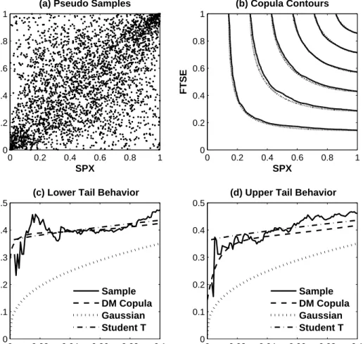
The pseudo-samples (Ut,Vt)are shown in Figure 3(a), which likes a scatter plot of Gaussian copula. The fitted Gaussian copula satisfies ˆρ=0.54. However, the fitted Gaussian copulaCNˆ
ρ is
not able to fit the tail parts. As is well known, the lower and upper TDC of Gaussian copula are both equal to zero. Hence in Figure 3(c), the valueCNˆ
ρ(x,x)/x tends to 0 when x approaches 0,
while the empirical data is obviously correlated in the tail parts. In conclusion, Gaussian copula fits the central part well but doesn’t fit the tail parts.
Next we use DMM to modify the tail parts of the fitted Gaussian copula. We choose Gaussian, Clayton and Gumbel copula as the component copulas, and chooseHf
α,β defined in equation (10)
as the distortion functions. According to Proposition3, the DM copula
CDmϑ (u1,u2) = (1−α2−α3)CρN(D(u1),D(u2)) +α2C Cl θ 1−Hf α2,β2(1−u1),1−H f α2,β2(1−u2) +α3CGuψ Hf α3,β3(u1),H f α3,β3(u2) (32)
0 0.2 0.4 0.6 0.8 1 0 0.2 0.4 0.6 0.8 1
(a) Pseudo Samples
SPX FTSE SPX FTSE (b) Copula Contours 0 0.2 0.4 0.6 0.8 1 0 0.2 0.4 0.6 0.8 1 0 0.02 0.04 0.06 0.08 0.1 0 0.1 0.2 0.3 0.4 0.5
(c) Lower Tail Behavior
Sample DM Copula Gaussian Student T 0 0.02 0.04 0.06 0.08 0.1 0 0.1 0.2 0.3 0.4 0.5
(d) Upper Tail Behavior
Sample DM Copula Gaussian Student T
Figure 3: (a) Pseudo-samples of daily log-return data (2000–2012) of S&P 500 and FTSE 100 In-dex. (b) Contour lines of empirical copula and the fitted DM copula. Solid lines belong to the em-pirical copula, and dotted lines belong to the fitted DM copula defined in (32) with parameter ˆϑ =
(0.54,0.02,0.10,0.56,0.02,5.0,1.1). (c) The valueC(u,u)/uof four copulas (u∈[0,0.1]). The fitted Gaus-sian copula has correlation parameter 0.54. The fitted Student T-copula has correlation parameter 0.54, and its freedom equals 2.7. (d) The value of ˆC(u,u)/u, where ˆCis the survival copula of corresponding copulas. has identical lower TDF with Clayton copulaCCl
θ and identical upper TDF with Gumbel copula CGuψ , where the parameterϑ = (ρ,α2,β2,θ,α3,β3,ψ)∈[0,1]×[0,12)×(0,∞)×[0,∞)×[0,12)× (0,∞)×[1,∞) and D(x) = (x−α2+α2Hαf2,β2(1−x)−α3Hαf3,β3(x))/(1−α2−α3). Since we regard the DM copulaCDm
ϑ as the tail modified version of the fitted Gaussian copulaC N
ˆ
ρ, we let
ρ=ρˆ =0.54.
We first setα2=α3=0.02, and the other four parameters are estimated by MLE. The estimates are ˆϑ = (0.54,0.02,0.10,0.56,0.02,5.0,1.1). Since the weight of component Gaussian copula α1 =96%, the fitted DM copulaCDmˆ
ϑ (u,v) is very close to the fitted Gaussian copulaC N
ˆ
ρ(u,v).
Actually, the mean difference ˆ 1 0 ˆ 1 0 C N ˆ ρ(u,v)−C Dm ˆ ϑ (u,v) dudv=0.0034,
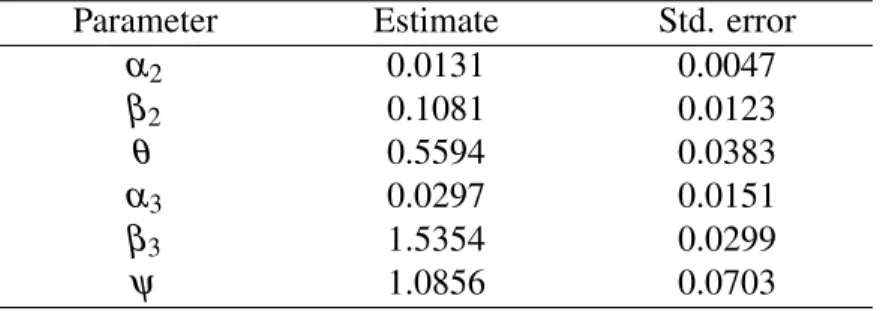
Table 1: Results of Maximum Likelihood Estimation. Parameter Estimate Std. error
α2 0.0131 0.0047 β2 0.1081 0.0123 θ 0.5594 0.0383 α3 0.0297 0.0151 β3 1.5354 0.0299 ψ 1.0856 0.0703
which is very small. However, as shown in Figure3(c)and Figure3(d), the DM copulaCDmˆ
ϑ fits the
empirical data very well in the tail parts. Comparing with the fitted Student T-copula, DM copula performs well both in the lower and upper tails. Therefore, DM copula shows a great flexibility in the results above, since its lower and upper tails can be calibrated separately.
In the next, we redo the calibration by MLE to estimate the weight parameters α2,α3. Ac-cording to the procedure in Section 2.4, we estimate the parameters ϑ = (ρ,α2,β2,θ,α3,β3,ψ) through the following steps.
• Step 1: We letρ equal the correlation parameter of the fitted Gaussian copula, i.e ρ=ρˆ =
0.54.
• Step 2: We expect sup(u,v)∈[0,1]2 C N ˆ ρ(u,v)−C Dm ϑ (u,v)
≤0.3. From Theorem1, we can set
α2,α3∈[0,0.05]in advance.
• Then we use MLE to calibrate(α2,β2,θ,α3,β3,ψ)with constraintsα2,α3∈[0,0.05]. The MLE estimate ˆϑml of ϑ is shown in Table 1, the values of ˆϑml have small changes to the
previous estimate ˆϑ discussed in Figure3, and the fitting effect is also similar.
In order to analyze the fitting effect in different regions, we consider square fit error in region
A⊆[0,1]2defined as eA(C) = 1 m(A) ¨ A |C(u,v)−Cemp(u,v)|2dudv 12 ,
in which m(A) is the Lebesgue measure of set A, C is a fitted copula andCemp is the empirical copula. The errors of different copulas in different regions are shown in Table2. From Table2, we can see that the fitted DM copulasCDmˆ
ϑ andC
Dm
ˆ
ϑml
perform better in tail parts (in region[0,0.05]2and region[0.95,1]2) than the fitted Gaussian copulaCNˆ
ρ. As for the central region[0.05,0.95]
2, the fit errors of DM copulas are close to the error of Gaussian copula. Hence these numerical results support our idea of constructing DM copulas to model the tail parts more accurately.
5
Conclusion
This paper introduced Distorted Mix Method (DMM) for constructing copula functions by combining the ideas of distortion and convex sum. The constructed DM copula can be very close
Table 2: Fit erroreA(C)of different fitted copulaCin different regions. Region CNˆ ρ C Dm ˆ ϑ C Dm ˆ ϑml [0,0.05]2 0.40% 0.06% 0.07% [0.95,1]2 0.35% 0.07% 0.06% [0.05,0.95]2 0.63% 0.70% 0.67% [0,1]2 0.58% 0.64% 0.62%
to a given copula and has tail dependence as desired. Theoretical properties of the DM copula were discussed by focusing on two tail dependence measures: tail dependence function and tail dependence coefficients of marginal distributions. As an application, a tight bound for asymptotic Value-at-Risk of order statistics was obtained under regular variation framework. Empirical results showed that DM copula fits the empirical data of SPX 500 Index and FTSE 100 Index very well both in central and tail parts.
Acknowledgments. The authors thank a referee for his valuable comments. The research of Kam C. Yuen was supported by a grant from the Research Grants Council of the Hong Kong Special Administrative Region, China (Project No. HKU 7057/13P), and the CAE 2013 research grant from the Society of Actuaries - any opinions, finding, and conclusions or recommendations expressed in this material are those of the authors and do not necessarily reflect the views of the SOA. The research of J. Yang was partly supported by the Key Program of National Natural Science Foundation of China (Grants No. 11131002) and the National Natural Science Foundation of China (Grants No. 11271033).
References
Caraux, G., Gascuel, O., 1992. Bounds on distribution functions of order statistics for dependent variates. Statistics & Probability Letters 14, 103–105.
Chen, X., Fan, Y., 2006. Estimation and model selection of semiparametric copula-based multi-variate dynamic models under copula misspecification. Journal of Econometrics 135, 125–154. Denuit, M., Dhaene, J., Goovaerts, M., Kaas, R., 2005. Actuarial Theory for Dependent Risks:
Measures, Orders and Models. John Wiley & Sons Ltd., Chichester.
Donnelly, C., Embrechts, P., 2010. The devil is in the tails: actuarial mathematics and the subprime mortgage crisis. ASTIN Bulletin 40, 1–33.
Durante, F., Foschi, R., Sarkoci, P., 2010. Distorted copulas: constructions and tail dependence. Communications in Statistics: Theory and Methods 39, 2288–2301.
Durante, F., Sempi, C., 2005. Copula and semicopula transforms. International Journal of Mathe-matics and Mathematical Sciences 2005, 645–655.
Fischer, M., Köck, C., 2012. Constructing and generalizing given multivariate copulas: a unifying approach. Statistics 46, 1–12.
Genest, C., Rivest, L.P., 2001. On the multivariate probability integral transformation. Statistics & Probability Letters 53, 391–399.
Hua, L., Joe, H., 2012. Tail comonotonicity: properties, constructions, and asymptotic additivity of risk measures. Insurance: Mathematics and Economics 51, 492–503.
Hull, J., White, A., 2004. Valuation of a CDO and an n-th to default CDS without Monte Carlo. The Journal of Derivatives 12, 8–23.
Joe, H., 1997. Multivariate Models and Dependence Concepts. Chapman & Hall, Boca Raton. Joe, H., Li, H., Nikoloulopoulos, A.K., 2010. Tail dependence functions and vine copulas. Journal
of Multivariate Analysis 101, 252–270.
Klement, E.P., Mesiar, R., Pap, E., 2005. Transformations of copulas. Kybernetika 41, 425–434. Klüppelberg, C., Kuhn, G., Peng, L., 2008. Semi-parametric models for the multivariate tail
de-pendence function: the asymptotically dependent case. Scandinavian Journal of Statistics 35, 701–718.
Li, D., 2000. On default correlation: a copula function approach. Journal of Fixed Income 9, 43– 54.
Liebscher, E., 2008. Construction of asymmetric multivariate copulas. Journal of Multivariate Analysis 99, 2234–2250.
Longin, F., Solnik, B., 2001. Extreme correlation of international equity markets. The Journal of Finance 56, 649–676.
McNeil, A.J., Frey, R., Embrechts, P., 2005. Quantitative Risk Management: Concepts, Techniques and Tools. Princeton University Press, Princeton.
Morillas, P.M., 2005. A method to obtain new copulas from a given one. Metrika 61, 169–184. Nelsen, R.B., 2006. An Introduction to Copulas, second edition. Springer, New York.
Rychlik, T., 1995. Bounds for order statistics based on dependent variables with given nonidentical distributions. Statistics & Probability Letters 23, 351–358.
Wang, S., 1996. Premium calculation by transforming the layer premium density. ASTIN Bulletin 26, 71–92.
A
The Proofs
Proof of Theorem1.According toAssumption A, it is easy to verify that ˜C(u1, . . .ud)has uniform [0,1] margins. To prove ˜Cis ad-dimensional copula function, we need to check thed-increasing property. Since everyDi j is increasing, the distorted component copulasCi(Di1(u1), . . . ,Did(ud))
are alld-increasing. Therefore, ˜Cis indeed a copula function.
The maximum difference betweenCandCican be estimated directly as sup (u1,u2,...,ud)∈[0,1]d C˜(u1,u2, . . . ,ud)−Ci(u1,u2, . . . ,ud) ≤ sup (u1,u2,...,ud)∈[0,1]d m
∑
k=1 αk|Ck(Dk1(u1), . . . ,Dkd(ud))−Ci(u1,u2, . . . ,ud)| ≤ sup (u1,u2,...,ud)∈[0,1]d αi|Ci(Di1(u1), . . . ,Did(ud))−Ci(u1,u2, . . . ,ud)|+∑
k6=i αk.By using the Lipschitz property of copula function,
sup (u1,u2,...,ud)∈[0,1]d αi|Ci(Di1(u1), . . . ,Did(ud))−Ci(u1, . . . ,ud)| ≤ d
∑
j=1 sup uj∈[0,1] αiDi j(uj)−αiuj = d∑
j=1 sup x∈[0,1] (1−αi)x−∑
k6=i αkDk j(x) ≤ d∑
j=1k∑
6=i αk· sup x∈[0,1] x−Dk j(x) ≤ d∑
j=1k∑
6=i αk.Combining all the inequalities above, we have
sup (u1,u2,...,ud)∈[0,1]d C˜(u1, . . .ud)−Ci(u1, . . . ,ud) ≤ d
∑
j=1k∑
6=i αk+∑
k6=i αk= (1−αi)(d+1),hence the proof of the inequality (2) is completed.
Before we prove theL1inequality in (3), we need to prove that ˆ 1 0 x−Di j(x) dx≤ 1 2 (33)
for anyiand j. Fixediand j, we denotey=Di j(12). Ify≥ 12, then ˆ 1 0 x−Di j(x) dx= ˆ 1 2 0 x−Di j(x) dx+ ˆ y 1 2 x−Di j(x) dx+ ˆ 1 y x−Di j(x) dx ≤ ˆ 1 2 0 (y−x)dx+ ˆ y 1 2 (1−x)dx+ ˆ 1 y (1−y)dx≤ 1 2.
For the casey< 12, we have similar argument to prove (33). By using (33), we have ˆ [0,1]d C˜(u1,u2, . . . ,ud)−Ci(u1,u2, . . . ,ud) du1. . .dud) ≤ ˆ [0,1]d m
∑
k=1 αk|Ck(Dk1(u1), . . . ,Dkd(ud))−Ci(u1,u2, . . . ,ud)|du1. . .dud ≤αi ˆ [0,1]d |Ci(Di1(u1), . . . ,Did(ud))−Ci(u1,u2, . . . ,ud)|du1. . .dud+ (1−αi) ≤ d∑
j=1 ˆ 1 0 αi Di j(x)−x dx+ (1−αi) = d∑
j=1 ˆ 1 0∑
k6=i αk x−Dk j(x) dx+ (1−αi) ≤d·∑
k6=i αk 2 + (1−αi) =d(1−αi)/2+ (1−αi),so the proof is completed.
Proof of Example2. According to Corollary1, we setS={1,2,3}in (27), then we getβ123≥0. And we obtainβ12≥β123 by settingS={1,2}in (27). Hence we haveβ23≥β123andβ13≥β123 by the same argument. Therefore, we know that 0≤β123≤min{β12,β23,β13}.
On the other hand, we set S={1} in (27), then we get 1−β12−β13+β123 ≥0. Next we set S={2} and S={3} again, we can derive β12+β23+β13−min{β12,β23,β13} −1≤β123. Combining these results, we obtain the inequalities in (28).
Proof of Theorem 4. Let i∗ =arg min1≤i≤k∑dj=−1k+iσδj/i, then we denote γ =∑d−k+i
∗
j=1 σδj/i∗=
min1≤i≤k∑dj=−1k+iσδj/i. Denote Fi,F(i) as the distribution functions of Xi,X(i) respectively. In the
next, we divide the proof into several steps.
Step 1. At first, we convert the conclusion into a distributional version. We will prove that max Xi∼µi+σi·X lim sup x→∞ ¯ F(k)(x)/F¯X(x) =γ (34) implies max Xi∼µi+σi·X lim sup α↓0 VaR1−α[X(k)] VaR1−α[X] =γ1/δ. (35)
Actually, if lim supx→∞F¯(k)(x)/F¯X(x)≤γ, combining with the assumption thatX varies regularly,
we derive that for anyε>0,
lim sup α↓0 ¯ F(k)(VaR1−α[X(k)]) ¯ FX(VaR1−α[X(k)]) ≤γ ≤γ+ε=lim α↓0 ¯ FX(VaR1−α[X]) ¯ FX((γ+ε)1/δVaR1−α[X]) . (36)
Then applying the fact limα↓0F¯(k)(VaR1−α[X(k)])/F¯X(VaR1−α[X]) =1, from (36) we know that
lim sup α↓0 ¯ FX(VaR1−α[X(k)]) ¯ FX((γ+ε)1/δVaR1−α[X]) ≥1,
which implies lim supα↓0(γ+ε)1/δVaR1−α[X]/VaR1−α[X(k)]≥1. Since ε is arbitrary, we can
conclude that lim supα↓0VaR1−α[X(k)]/VaR1−α[X]≤γ1/δ. Furthermore, by the same argument,
if a random vector (X1, . . . ,Xd) satisfies limx→∞F¯(k)(x)/F¯X(x) = γ, we can also conclude that
limα↓0VaR1−α[X(k)]/VaR1−α[X] =γ1/δ. Hence we have proved that (34) implies (35), so in the
following we will prove (34).
Step 2. DenoteCas the survival copula ofX1, . . . ,Xd. We will prove lim x→∞ ¯ F(k)(x)/F¯X(x) =
∑
S⊆D,|S|≥k eS(σ1δ, . . . ,σdδ;C). (37)According to the definition ofeS(σ1δ, . . . ,σdδ;C)in (17), we have
∑
S⊆D,|S|≥k eS(σ1δ, . . . ,σdδ;C) =∑
S⊆D,|S|≥k lim x→∞P \ i∈S {F¯i(Xi)≤σδ i F¯X(x)} \ j∈/S {F¯j(Xj)>σδ jF¯X(x)} /F¯X(x). (38)On the other hand, it is easy to verify that
lim x→∞ ¯ F(k)(x)/F¯X(x) =
∑
S⊆D,|S|≥k lim x→∞P \ i∈S {Xi≥x}\ j∈/S {Xj<x} /F¯X(x). (39) Comparing (38) with (39), we can derivelim x→∞ ¯ F(k)(x) ¯ FX(x) −
∑
S⊆D,|S|≥k eS(σ1δ, . . . ,σdδ;C) ≤∑
S⊆D,|S|≥k lim x→∞ ∑di=1P {Xi≥x}∆{F¯i(Xi)≤σiδF¯X(x)} ¯ FX(x) =∑
S⊆D,|S|≥k lim x→∞ d∑
i=1 ¯ Fi(x) ¯ FX(x) −σiδ =0, where the last equality is due tolim x→∞ ¯ Fi(x)/F¯X(x) = lim x→∞ ¯ FX( x−µi σi )/F¯X(x) =σiδ, i=1, . . . ,d. (40)
Hence the equality in (37) has been proved.
Step 3. We will prove that
lim
x→∞
¯
F(k)(x)/F¯X(x)≤γ. (41)
LetCbe the survival copula ofX1, . . . ,Xd. Recall the supplementary definitionb(wi;C{i}) =wifor
i=1, . . . ,d. According to the conclusion in (18), we know that
σiδ =b(σiδ;C{i}) =
∑
S⊆D,i∈STherefore, for anyi∈ {1, . . . ,k}, 1 i d−k+i
∑
j=1 σδj =1 i d−k+i∑
j=1 S⊆∑
D,i∈S eS(σ1δ, . . . ,σdδ;C) =1 i∑
S⊆D,S6=/0 eS(σ1δ, . . . ,σdδ;C)× |S∩ {1,2, . . . ,d−k+i}| =1 i S⊆∑
D,S6=/0 eS(σ1δ, . . . ,σdδ;C) (|S|+d−k+i− |S∪ {1,2, . . . ,d−k+i}|) ≥1 i∑
S⊆D,S6=/0 eS(σ1δ, . . . ,σdδ;C) (|S|+d−k+i−d) ≥∑
S⊆D,|S|≥k eS(σ1δ, . . . ,σdδ;C)(|S|+i−k) i ≥∑
S⊆D,|S|≥k eS(σ1δ, . . . ,σdδ;C) = lim x→∞ ¯ F(k)(x)/F¯d(x),where the last equality is owing to (37). By the definition γ =min1≤i≤k∑dj=−1k+iσδj/i, we obtain
(41).
Step 4. We will prove the bound in (41) is tight. Settingwi=σiδ fori=1, . . . ,dand using the
parameters defined in (30),(31), we construct DM copulas ˜Cby (21) in Theorem3. Next we will prove if the survival copula ofX1, . . . ,Xd is the DM copula ˜C, then the upper bound in (41) holds.
Firstly, we prove that
σ1δ ≤. . .≤σdδ−k+i∗ ≤γ (42)
and
γ ≤σdδ−k+i∗+1≤. . .≤σdδ wheni∗<k. (43)
Recall the assumption σ1≤. . . ≤σd. For the case i∗<k, the definition γ =∑d−k+i
∗
j=1 σδj/i∗ =
min1≤i≤k∑dj=−1k+iσδj/iimplies that
d−k+i∗+1
∑
j=1
σδj
i∗+1 ≥γ,
this inequality can be simplified asγ≤σdδ−k+i∗+1, hence (43) holds. On the other hand, fori∗>1, by the definition ofγ, we also know
d−k+i∗−1
∑
j=1
σδj
i∗−1 ≥γ,
which implies γ ≥σdδ−k+i∗. And if i∗ =1, then γ =∑dj=−1k+1σδj ≥σdδ−k+1. Therefore, we have
proved (42).
Secondly, we will prove that for any x∈[0,γ), x exactly belongs to different i∗ sets among
{R1, . . . ,Rd−k+i∗}. Recall the definitionsγ=∑d−k+i
∗ j=1 σδj/i∗andRi= h ∑ij=−11σjδ,∑ij=1σδj (modγ)
fori=1, . . . ,d−k+i∗. Thus, for anyx∈[0,γ), thei∗numbers {x,x+γ,x+2γ, . . . ,x+ (i∗−1)γ} ⊆[0,i∗γ) = d−k+i∗ [ i=1 h ∑ij=−11σjδ,∑ij=1σδj .
Owing to the result in (42), the length of each interval among nh
∑ij=−11σjδ,∑ij=1σδj
: i=1, . . . ,d−k+i∗o (44) is smaller thanγ. Hence thei∗numbers{x,x+γ,x+2γ, . . . ,x+ (i∗−1)γ}belong to different i∗
intervals among (44). SinceRi=h∑ij=−11σδj,∑ij=1σδj
(modγ)fori=1, . . . ,d−k+i∗, we conclude
that for anyx∈[0,γ),xexactly belongs to differenti∗sets among{R1, . . . ,Rd−k+i∗}.
On the other hand, combining the result in (43) with the definitionRi= [0,σiδ),i=d−k+i∗+
1, . . . ,d, we know that[0,γ)⊆Rifor anyi∈ {d−k+i∗+1, . . . ,d}. So for anyx∈[0,γ),xexactly
belongs to differentksets among{R1, . . . ,Rd}, which implies [0,γ)⊆ [ S⊆D,|S|=k T i∈SRiTj∈/SRcj ⊆ [ S⊆D,|S|≥k T i∈SRiTj∈/SRcj . (45)
Note that∩i∈SRi∩j∈/SRcjis pairwise disjoint forS⊆D,S6= /0. Combining with the definition ofµS
in (31), we have
∑
S⊆D,|S|≥k µS=∑
S⊆D,|S|≥k ml T i∈SRiTj∈/SRcj ≥ml( [0,γ) ) =γ. (46)As the proof of Theorem3part (I), we know thatµS=eS(σ1δ, . . . ,σdδ; ˜C)forS⊆D,S6=/0 by setting wi=σiδ,i=1, . . . ,d and comparing the definition in (20) with the expression in (19), Therefore,
from (37) we obtain lim x→∞ ¯ F(k)(x)/F¯d(x) =
∑
S⊆D,|S|≥k eS(σ1δ, . . . ,σdδ; ˜C) =∑
S⊆D,|S|≥k µS≥γ. (47)Combining the above results in Step 1 to Step 4, from (41) and (47) we get limx→∞F¯(k)(x)/F¯X(x) =
![Table 2: Fit error e A (C) of different fitted copula C in different regions. Region C N ˆ ρ C Dmˆ ϑ C Dmˆϑ ml [0, 0.05] 2 0.40% 0.06% 0.07% [0.95, 1] 2 0.35% 0.07% 0.06% [0.05, 0.95] 2 0.63% 0.70% 0.67% [0, 1] 2 0.58% 0.64% 0.62%](https://thumb-us.123doks.com/thumbv2/123dok_us/1181018.2658485/20.918.228.694.153.291/table-different-fitted-copula-different-regions-region-dmˆϑ.webp)
