Abstract: In this work, the objective is to classify the audio data into specific genres from GTZAN dataset which contain about 10 genres. First, it perform the audio splitting to make it signal into clips which contains homogeneous content. Short-term Fourier Transform (STFT), Mel-spectrogram and Mel-frequency cepstrum coefficient (MFCC) are the most common feature extraction technique and each feature extraction technique has been successful in their own various audio applications. Then, these feature extractions of the audio fed to the Convolution Neural Network (CNN) model and VGG16 Neural Network model, which consist of 16 convolution layers network. We perform different feature extraction with different CNN and VGG16 model with or without different Recurrent Neural Network (RNN) and evaluated performance measure. In this model, it has achieved overall accuracy 95.5\% for this task.
Keywords : GTZAN, Short-term Fourier Transform (STFT), Mel-spectrogram, Mel-frequency cepstrum coefficient (MFCC), Convolution Neural Network, VGG16, Recurrent Neural Network (RNN)
I. INTRODUCTION
Today we know, data are increasing exponentially over the years. So, result in analysis of the data are getting difficult and taking too long time to get task done. Specifically, for audio data, which contains large amount of sampling data (around 660,000) for duration of 30 seconds. In the real-time, like Saavn, which have over 5 crore audio data or music and all audios have also been categorized into different genre. Here, Data play vital role as a computer science or data science. “Music” is also considered as a part of life. Whenever people work, or coming from office, or any other activity, the music gives us to relax our mind and make our soul to high spirit. Music also make us creativity and motivation when people are in sad mood or depression. Once you start listening to music, all the pain or stressing on our brain make you forget them and bring you into high spirit like confidence, no feeling stress, peaceful while mediation, etc.
“Genre”, as per dictionary, means categories of music. It also important to categorize the music into different part of music that they belong. For example, if you are in party, the music will be played related to rock or jazz genre. If you are doing aerobics or exercise part, then music will be played
Revised Manuscript Received on November 05, 2019.
Faiyaz Ahmad, Computer Engineering, Jamia Millia Islamia, New Delhi, India. Email: [email protected]
Sahil,, Computer Engineering, Jamia Millia Islamia, New Delhi, India. Email: [email protected]
related to theme genre. So, music genre brings us which nature of music we like to listen.
Nowadays, you will find music websites or app from smartphone like Saavn, Gaana, JioSavan, etc contains 50 million and with 15 different languages present in it. Most of the people are also remaking the combination of two songs, which called as MASHUP, to make to mix of these songs. So, more music or audios data are creating for the entertainment to the people. So, if we make a different genre for every music as which type of nature of songs it is. It would help people to find that song or genre they want to listen. Without that, it‟s would never know what type of song or music it is, like is it mediation or pop songs? To do that, we listen to every music and make a list of genres they belong, which is very time consuming. So, Music Genre also play important of the life and entertainment to the people which can enjoy with the fullest.
II. RELATEDWORKS
Various papers have been published regarding the music genre classification. These techniques primarily used various feature extraction methods and then apply classifiers to classify the audio into specific genre. Some of them used Machine Learning and Deep Learning-Based approaches. Caifeng Liu et al. [1], they proposed new develop convolution neural networks architecture which takes the long related to context of information into considerations and transfers further suitable information to decision-making layer. To develop the new neural network, they used the idea of Inception model by combine convolutions with different kernel size and layers. So, the dataset they used were GTZAN, Ballroom and Extended Ballroom. The pre-processing steps done to extract feature called mel-spectogram with 128 Mel filters from audio signal. Then this feature input of size 647x128 fed to BBNN. They achieved overall accuracy 93.9%, 96.7%, 97.2%.
Prasenjeet Fulzele et al. [2], they implemented this proposed model into two parts. First, features were extracted from the audio files and arranged them such a manner that they fed to two models. Secondly, they involved fusion of two models by sum rule. To predict the final prediction, the separate posterior probabilities have combined them to get result. In this work, the dataset they used GTZAN dataset.
Music Genre Classification using Spectral
Analysis Techniques With Hybrid
Convolution-Recurrent Neural Network
They were extracted 9 features from audio file in order to see the audio pattern by machine learning algorithm. Now these inputs are trained into two model individually and then merge them to get final prediction result. Hyperparameter was used by Random Grid Search. They achieved with the overall accuracy of 89% by combining SVM and LSTM model. Nilesh M. Patil et al. [3], they had done with the idea of applying Machine Learning Techniques. SVM and k-NN are the most frequent applied machine learning techniques in many fields like image processing, twitter sentimental analysis, etc. In this work, the dataset they used GTZAN. To obtain the feature extraction from the audio file, it‟s done by Mel-Frequency Cepstral Coefficients (MFCC), then feature vectors are obtained. Now, these feature vectors are classified with supervised learning approaches i.e. k-NN, Linear SVM and Poly SVM. Each classifier have achieved overall accuracy with 64.4%, 60% and 77.78%.
Ahmed Elbie et al. [4], the GTZAN dataset is used and perform feature extraction is statistical descriptors. They extracted about 8 features i.e. zero crossing rate, spectral centroid, spectral contrast, spectral bandwidth, spectral roll off and MFCC. Each feature is evaluated with different machine learning techniques and then also same techniques was done with combined features one. It found that SVM had perform better with combined features which achieved 72%. Further, it extended to work with applying deep learning algorithm in audio which was Convolution Neural Network (CNN). Before fed to the network, they perform with 3 parts: raw data, STFT with hop length 1024 and window size 2048 and MFCC with 13 coefficients. It found that it achieved 66% accuracy.
Pradeep Kumar D et al. [5], they study to detect and classify GTZAN audio files and then compare them by using various classification algorithms. For feature extraction, they used Fast Fourier Transform (FFT) and Mel Frequency Cepstral Coefficients (MFCC). Logistic Regression, Support Vector Machines, Decision trees, K-NN, Recurrent Neural Network were used as the classifier algorithms. When apply Recurrent Neural Network, they achieved highest accuracy among the others with 86%.
Anshuman Goel et al. [6], they used 8 feature extraction from the audio file, that is, beat periodicity, loudness, energy, speechness, acousticness, valence, danceability, discrete wavelet transform (DWT). Then these features are fed to the neural network. They done with the 2 genres only, Classical and Sufi songs. They achieved with the accuracy of 85% testing. Classical songs correctly predicted with overall 87% of data and Sufi songs correctly predicted with overall 82% of data.
Jan Jakubik [7], they performed with two Recurrent Neural Network (RNN): LSTM and GRU. They experiment on 4 datasets: GTZAN, Emotify, Ballroom and LastFM. The spectrogram were used as the feature extraction. It compares all datasets with LSTM and GRU train and test. The GRU has been performed better than LSTM with the overall 92% accuracy and for LSTM, the overall accuracy 89% accuracy. George Tzanetakis [8], three feature set are applied, i.e., timbral texture, rhythmic content and pitch content and the statistical pattern recognition classifier is used , i.e.. Gaussian Mixture Model (GMM), k-Nearest neighbor (kNN) and simple Gaussian (GS). They used GTZAN dataset and real time-based music. It has achieved with overall 61% accuracy to real time music.
Lin Feng et al. [9], they proposed hybrid model which consist of Convolution Neural Network and Bi-RNN parallel to other. GTZAN dataset used in this paper. They used short term fourier transform feature extraction technique with frame number 1024 with 50% overlapping. It proved that CNN working RNN can improved with achievement of 92% accuracy.
III. PROPOSEDWORK
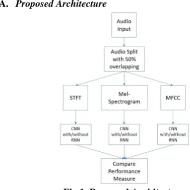
[image:2.595.306.498.171.363.2]A. Proposed Architecture
Fig 1. Proposed Architecture
B. Dataset
It performs on GTZAN [18] dataset. It contains 10 classes and each class contains 100 audios. Each audio contains 30 seconds of track. The tracks are in 22050 Hz with mono 16-bit audio file in .wav format. Below table are the class list name of the music.
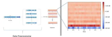
C. Data-Preprocessing
An audio read with the sampling rate of 22050 Hz. After that, it split the audio of 30 seconds durations into 3 seconds durations of audio clips. The problem is that when split the audio, the computer will consider that each clip is not relate to each other and are independent. So, in order to avoid this, 50\% of previous duration of data is taken and append with next 50\% of next duration of data. This will help to understand the computer and maintain consistent that the first 50\% duration of data are from the previous audio clip and from that data, it continues to next 50% duration of data.
D. Feature Extraction Used
Each clip has performed different feature extraction to see the analysis which one been performed better.
1. Short-Term Fourier Transform (STFT)
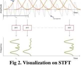
Due to the lack of fundamental tradeoff between time and frequency, it used short-term Fourier transform \cite{s1}. As the name suggested “short term” means signal are split into small fixed duration of signal and then apply Fourier transform of each block. Moving the sliding to create every block in signal called framing. This is computed frequency change with signal over time. Before computing, each block is multiplied with windowing function in order to enhance the ability of Fourier Transform to extract spectral data from signals. It used Hann window which look like a bell curved shape (see function g(t) in fig
After finding the Fourier transform of each signal, the result will get in complex number. To bring into real number, it evaluate their absolute value of that complex number. Now after applying (Fast Fourier Transform) FFT on each block, the resultant called frequency representation. Now this all frequency representation with time for this signal will be consider as their features which is also called as spectrogram.
Fig 2. Visualization on STFT
[image:3.595.88.250.139.270.2]So, when it applied Short Term Fourier Transform (STFT) on each clip where FFT window size (frame size) is 1024 and hop length (frame increment) is 512 and windowing function is Hann function. Each clip gets (513, 129) dimensions that is 513 frequency bins and 129 frames in time.
Fig 3. STFT Spectrum for a blue class audio with 3 seconds duration
2.Mel-Spectrogram
Mel-Spectrogram [20] is the part of digital filter bank. Digital filter bank is a set of bandpass filters for a single input.
Fig 4. Analysis Part of Digital Filter Bank where x(t) is an input signal, 'n' is number of filter bank analysis, A(f) is analysis filter. By using these, a signal can decomposed into different sub band signal occupying a portion of the original frequency band.
In similar fashion, (in Fig 4.), its exactly looks like analysis part of digital filter bank till Mel Filter Bank in Fig 5. First thing is, it take audio as an input and then, framing the audio with window size done to get samples into the buffer block and apply Window block (e.g. Hann windows) and then perform Fast Fourier Transform (FFT Block) which is convert time domain signal into frequency domain. This process is performed same as STFT technique.
Fig 5. Procedure of evaluating Mel-Spectrogram To further extend, this frequency domain of signal is passed through every analysis filter bank which is Mel-Spaced Filter Bank. To calculate the filter bank energy, a signal is multiplied with the filter bank and are summed up with their coefficient and every summed coefficient with „n‟ filters are created vectors of Mel Spectrogram. That is, for each frame of the signal, we get „n‟ vector of Mel-Spectrogram.
Mel Filter Bank is calculated by
[image:3.595.68.269.344.406.2]where „n‟ is number of filter bank we want and “frbin()” is the list of frequencies bins and „z‟ is the list of natural number up to maximum of frequencies bin. When this equation is applied, the resultant value get the triangular graph (See in Fig. 6). Each color of triangle represents different analysis filter bank. And this can compare this filter band in this graph (Fig 6.) to Mel-Filter Bank (in Fig 5.). So, each triangle filter taken as different blocks. For example, in Fig 5., blue triangle part at starting is taken as first block, next orange triangle part is taken as second block and so on till „n‟ triangle part is taken as „n‟ block.
Fig 6. MelBank Filter when n=10
[image:3.595.341.514.479.540.2]When it applied Mel-Spectrogram on each clip where FFT window size is 1024 and hop length is 512. Each clip gets (128,129) dimensions (in fig 7.).
Fig 7. Mel-Spectrogram for a blue class audio with 3 second duration
3.Mel-Frequency Ceptrum Coefficient (MFCC)
It is further extension of Mel spectrogram. Mel-Frequency Cepstral Coefficient [20] is another representative way of spectrum of the audio clip, after compressing the frequency. From the mel frequencies output in Mel spectrogram, we take the log of the power and then chose first 13-20 coefficient
after Discrete Cosine
[image:3.595.90.243.486.603.2] [image:3.595.328.525.593.652.2]Increasing number of coefficients represent the incremental changes in estimated energy, thus they got less data. Of course, the most information lost that why it said this technique used for audio compression. Then, apply DCT instead of Taking inverse fast Fourier transform (FFT) because it is most likely perform same as FFT and it is also easy to compute and implement.
Fig 8. Procedure of evaluating MFCC
[image:4.595.315.540.162.224.2]When it applied further extended to Mel-Spectrogram to MFCC. With different top k coefficient values after applying DCT, k = 13 has got to be the best optimal choice.
Fig 9. MFCC for a blue class audio with 3 seconds duration
E. Learning Algorithm
Data are divided into three sections: training data, validation data and test data. And these data are split into 80% of training data, 10% of validation data and 10% of testing data. Clips can be shuffled, there is no issue and loss of series because each clip have retained 50% previous data, so they are all connected with other clips which done in data preprocessing stage. These training data are then fed to Hybrid Convolution-Recurrent Neural Network before reshaping the data. Once an epoch is done, it check the performance of validation data to see how much can generalize the unknown data after learnt from training data. Once it completed all trained network, evaluation for the test data is done after seeking training and validation data performance.
Applying Convolution Neural (CNN) has given the promising and better result in image classification and recognition. So, all features are treated as images feature to recognition the pattern using CNN model which will given better performance result and CNN also consider as a self feature learning, i.e., while performing convolution to that images, it gets the various feature with different convolution kernel filter. VGG16 [12] ,which consists of 16 layers of CNN, has been trained on Mel-Spectrogram feature extraction data only because of the limited resource present in our system. This network has outperformed than CNN in these features. You will see the result in tabular form clearly in the next section part.
Since, in traditional deep learning, the weight and bias of hidden layer are different from each other that why they are independent and can‟t be combined to work together. In order to combine hidden layers, they need to consider as same weight and bias for these hidden layers. To overcome this issue, Recurrent Neural Network (RNN) [13] plays roles which retain some of the memory store for future references. Due to some limitation [14], variant of RNN are applied: Long Term Short Model (LSTM) [15][19], Gate Recurrent Units (GRU) [16] and Bi-Directional RNN (Bi-RNN) [17].
We have trained the network model with CNN model with or without RNN model. While training the model, several tuning hyperparameters has been done and try to obtain best performance as possible.
[image:4.595.72.263.257.320.2]In this proposed CNN architecture, we create five Convolution Block layer. Each block layer contains Convolution Kernel with different kernel size followed by MaxPooling Layer followed by Dropout with droprate 25%. Then flatten them into 1D array and output layer. (see Fig 10.)
Fig 10. Proposed CNN Architecture
[image:4.595.327.530.317.387.2]And for proposed CNN with LSTM (or GRU) architecture, we create five Convolution Block layer. After that we followed by three LSTM (or GRU) layer with two 128 LSTM (or GRU) units and one 64 LSTM (or GRU) unit then we flatten them into 1D array and apply one dense layer and finally, that last one as, output layer. (see Fig 11.)
Fig 11. Proposed CNN with LSTM (or GRU) Architecture
And for CNN with Bi-LSTM (or Bi-GRU), we create four Convolution Block layer. After that we followed by one LSTM (or GRU) layer with one 128 LSTM (or GRU) unit followed by bi-Directional LSTM (or Bi-GRU) layer with 128 units followed by one 64 LSTM (or GRU) units then flatten them into 1D array and apply one dense layer and finally, that last one as, output layer (see Fig 12.).
Fig 12. Proposed CNN with Bi-LSTM (or Bi-GRU) Architecture
F. Result with different feature extraction and learning
algorithm used
Table 1. Performance Evaluation and Result
STFT CNN 70 0.9598 0.9485 0.955
STFT CNN+LSTM 70 0.9283 0.9117 0.922
STFT CNN+GRU 70 0.9227 0.9193 0.928
STFT CNN+Bi-GRU 50 0.9041 0.9041 0.902
STFT CNN+Bi-LSTM 120 0.7723 0.773 0.773
Mel-Spectrogram CNN 120 0.8788 0.9023 0.901
Mel-Spectrogram CNN+LSTM 120 0.9214 0.914 0.903
Mel-Spectrogram CNN+GRU 120 0.9186 0.9187 0.904
Mel-Spectrogram CNN+Bi-LSTM 120 0.9273 0.9041 0.895
Mel-Spectrogram CNN+Bi-GRU 120 0.9254 0.9041 0.895
Mel-Spectrogram VGG16 25 0.9831 0.9351 0.919
Mel-Spectrogram VGG16+LSTM 20 0.9335 0.8719 0.877
Mel-Spectrogram VGG16+GRU 20 0.9551 0.8877 0.884
Mel-Spectrogram VGG16+Bi-GRU 20 0.9457 0.886 0.892
Mel-Spectrogram VGG16+Bi-LSTM 15 0.8528 0.8339 0.803
MFCC CNN 200 0.8949 0.8491 0.862
MFCC CNN+LSTM 200 0.8559 0.8474 0.853
MFCC CNN+GRU 200 0.8331 0.8281 0.831
MFCC CNN+Bi-LSTM 200 0.8616 0.8509 0.852
MFCC CNN+Bi-GRU 200 0.8601 0.8 0.791
G. Graph Between Training Data and Validation Data
with respect to Accuracy and Loss
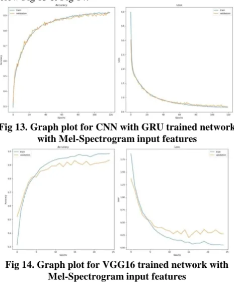
[image:4.595.318.536.476.527.2] [image:4.595.310.556.579.713.2]For Mel-Spectrogram Feature extractions data, it performed on two networks (CNN and VGG16). Graph plots are shown below Fig 13 & Fig 14.
Fig 13. Graph plot for CNN with GRU trained network with Mel-Spectrogram input features
Fig 14. Graph plot for VGG16 trained network with Mel-Spectrogram input features
[image:5.595.52.285.83.363.2] [image:5.595.46.289.378.527.2]For MFCC feature extraction data, graph plot is shown below (Fig 15).
Fig 15. Graph plot for CNN trained network with MFCC input features
For STFT feature extraction data, graph plot is shown below (Fig 16).
Fig 16. Graph plot for CNN trained network with STFT input features
H. Compare with other research work
Table 2. Comparison with other research Author Name Accuracy (%)
Caifeng Lui et al.[1] 93.9
Praseneet Fulzeele et al.[2] 89 Nilesh M. Patil et al.[3] 77
Ahmad Elbir et al.[4] 72
Pradeep Kumar D et al.[5] 86
Jan Jakubik [7] 92
George Tzanetakis [8] 61
Lin Feng et.al.[9] 92
Proposed Work 95.5
IV. CONCLUSION
In this work, we have performed with new terminology called audio split. Due to rate of change of every signal was changing every interval of time. To overcome that, we split an audio of 30 seconds into clips with 3 seconds duration and 50\% overlapping with previous signal to remain dependent. Then we performed three spectral analysis feature extraction techniques which has been performed for several applications related music and speech are Short term Fourier Transform (STFT), Mel-Spectrogram and Mel-Frequency Cepstral Coefficients (MFCC). And train the network with combining Convolution Neural Network with Recurrent Neural Network in order to achieved better performance measure. We achieved 96\% training accuracy, 95\% valid accuracy and 95.5\% percent test accuracy using short term fourier transform (STFT) with Convolution Neural Network (CNN).
REFERENCES
1. Caifeng Liu, Lin Feng, Guochao Liu, Huibing Wang, Shenglan Liu,” Bottom-up Broadcast Neural Network For Music Genre Classification”, ScienceDirect,Elsevier,Pattern Recognition, Jan, 2019.
2. Prasenjeet Fulzele, Rajat Singh, Naman Kaushik, Kavita Pandey,” A Hybrid Model For Music Genre Classification”, Proceedings of 2018 Eleventh International Conference on Contemporary Computing (IC3), Aug, 2018.
3. Nilesh M. Patil, Dr. Milind U. Nemade,” Music Genre Classification Using MFCC, K-NN and SVM Classifier”, International Journal Of Computer Engineering In Research Trends, Vol. 4, Issue. 2, Feb, 2017. 4. Ahmed Elbir, Hilmi Bilal Cam, Mehmet Emre lyican, Berkay Ozturk, Nizamettin Aydin,” Music Genre Classification and Recommendation by using Machine Learning Techniques“,Innovations in Intelligent Systems and Applications Conference, Oct, 2018.
5. Pradeep Kumar D, Sowmya B. J., Chetan, and K. G. Srinivasa ,” A Comparative Study of Classifiers for Music Genre Classification based on Feature Extractors”, IEEE Distributed Computing, VLSI, Electrical Circuits and Robotics, Aug, 2016.
6. Anshuman Goel, Mohd. Sheezan, Sarfaraz Masood, Aadam Saleem,” Genre Classification of Songs Using Neural Network”, International Conference on Computer and Communication Technology (ICCCT), Sept, 2014.
7. Jan Jakubik,” Evaluation of Gated Recurrent Networks in Music Classification Tasks”, Information System Arxhitecture and Technology: Proceedings of 38th International Conference on Information Systems Architecture and Technology, 2017.
8. George Tzanetakis,” Musical Genre Classification of Audio Signals”, IEEE Transactions on Speech and Audio Processing, July, 2002. 9. Lin Feng, Shenlan Liu, Jianing Yao,” Music Genre Classification with
Paralleling Recurrent Convolutional Neural Network”, arXiv, Dec, 2017.
11. Rikiya Yamashita, Mizuho Nishio, Richard Kinh Gian Do, Kaori Togashi,” Convolution Neural Network: an overview and application in radiology”, Springer, Volume 9, Issue 4, Aug, 2018.
12. Keren Simonyan and Andrew Zisserman,” Very Deep Convolution Networks For Large Scale Image Recognition”, ICLR 2015.
13. Alex Graves and Navdeep Jaitly,” Towards End-to-End Speech Recognition with Recurrent Neural Networks”, Proceedings of the 31st International Conference on Machine Learning, vol 32, 2014. 14. Yoshua Bengio, Patrica Simard and Paolo Fransconi,” Learning
Dependencies with Gradient Descent is Difficult”, IEEE Transactions On Neural Networks, Vol 5, No 2, Mar, 1994.
15. Sepp Hochreiter, Jurgen Schmidhuber,” Long Short-term Memory”, Neural Computation, 1997.
16. Yoshua Bengio, Cho et. al,” Learning Phase Representation using RNN Encoder-Decoder for Statistical Machine Transalation”, arXiv, Sept, 2014.
17. Mike Schuster and Kuldip K. Paliwal,” Bidirectional Recurrent Neural Networks”, IEEE Transactions on Signal Processing, vol 45, no. 11, 1997.
18. Bob L. Strum,” The GTZAN dataset: Its contents, its faults, their effects on evaluation, and its future use”, arXiv, Jun, 2013
19. Understanding LSTM network, Available at:
https://colah.github.io/posts/2015-08-Understanding-LSTMs/
20. Mel Frequency Ceptral Coefficient (MFCC) tutorial, Available at:
http://practicalcryptography.com/miscellaneous/machine-learning/guid e-mel-frequency-cepstral-coefficients-mfccs/
AUTHORSPROFILE Faiyaz Ahmad, Faiyaz Ahmad, Assistant professor, Department of computer Engineering ,Jamia Millia Islamia, New Delhi, India
Sahil, done Master of Technology in Computer Engineering from Jamia Millia Islamia and is currently pursing on Data Scientist or Machine Learning Engineering. He has been reading several researches on Deep Learning and Image Processing to get the more depth knowledge and understanding on how model and feature extraction on specific problem works behind.