Aerial Object Detection using Learnable Bounding Boxes

Rochester Institute of Technology

RIT Scholar Works

Theses

2-2019

Aerial Object Detection using Learnable Bounding

Boxes

Aneesh Bhat

[email protected]

Follow this and additional works at:https://scholarworks.rit.edu/theses

This Thesis is brought to you for free and open access by RIT Scholar Works. It has been accepted for inclusion in Theses by an authorized administrator of RIT Scholar Works. For more information, please [email protected].

Recommended Citation

Aerial Object Detection using Learnable

Bounding Boxes

by Aneesh Bhat February 2019

A Thesis Submitted in Partial Fulfillment

of the Requirement for the Degree of Master of Science

In

Aerial Object

Detection using

Learnable Bounding

Boxes

Aneesh Bhat February

2019

KATE GLEASON COLLEGE OF ENGINEERING A Thesis Submitted in Partial

Fulfillment

of the Requirements for the Degree of Master of Science in

Computer Engineering

i

Aerial Object Detection using Learnable

Bounding Boxes

By

Aneesh Bhat

February 2019

A Thesis Submitted in Partial Fulfillment of the Requirements for the Degree of Master of Science

in Computer Engineering from Rochester Institute of Technology

Approved by:

Dr. Raymond Ptucha, Assistant Professor Date

Thesis Advisor, Department of Computer Engineering

Dr. Clark Hochgraf, Associate Professor Date

Thesis Advisor, Department of Electrical Engineering

Dr. Alexander Loui, Associate Professor Date

Committee Member, Department of Electrical Engineering

Department of Computer Engineering

ii

Abstract

iii

Contents

Signature Sheet……… i

Abstract………... ii

Table of Contents………... iii

List of Figures………..……. vii

List of Tables………...… x

Acronyms………...…… xi

I

Object Detection Networks

Chapter 2: Related Work……….………...… 3

Chapter 3: YOLO - You Only Look Once………..………...… 5

3.1 Background……….... 5

3.2 Overview of the YOLO Pipeline………... 6

3.3 Non-Max Suppression………...……… 9

3.4 Deficiencies of YOLO………..………. 11

Chapter 4: YOLO v2- Better, Stronger, Faster………..…...… 13

4.1 Introduction………... 13

4.2 Changes from YOLO……….... 15

Chapter 5: YOLO v3………... 20

iv

5.2 Overview of YOLO v3………...……... 20

5.3 Backbone Architecture………...………... 23

Chapter 6: Applications of YOLO………..……… 29

6.1 Object Detection Networks………... 29

6.2 YOLO in Aerial Imaging…..………..………... 30

6.3 Shortcomings of YOLO……….………... 31

II

Methodology

7.1 Experiment Methodology………...………….…………...….... 32

7.2 DOTA Dataset…...……….….………... 32

7.3 Data Preprocessing……….………... 34

7.4 Incorporating Angle to Annotations.………....….……….…... 36

Chapter 8: Rotating Anchor Boxes………...………….……….…... 40

8.1 Rotated Anchor Boxes………....…...………….…………...…... 40

8.2 Activation of Angle………...………….………..…...…... 40

8.3 Angle Loss.………...…………...…………...…... 41

8.4 IOU of Boxes………...………….…………...…... 43

8.5 Evaluating the model………...………….…………...…... 43

Chapter 9: Rotating Anchor Boxes………....………….………... 46

9.1 Anchor Box and Wiggle Tradeoff.………...………….…………...…... 46

v

9.3 Wiggle for Anchor Boxes………...………….…………...…... 47

9.4 Training Specifications.………...…...……….…………...…... 48

Chapter 10: Rotating Anchor Boxes………...………...….………... 49

10.1 Shortcomings of Rotated Anchor Boxes.……….………...…...…... 49

10.2 Selection of Anchor Box.………...………….…………...…... 49

10.3 Activation Function for Point Values.………...………….…………...…... 50

10.4 Calculating IOU.………...………….………...…...…... 53

10.5 Loss Function for Deformable Point Network.…………...…………....…………...…... 54

Chapter 11: Rotating Anchor Boxes………...………….……...…………... 55

11.1 Motivation and Objective.………...…...……….…………...…... 55

11.2 Training Scheme.………...………….…...………...…... 55

11.3 Testing.………...………….………...…...…... 56

11.4 Experiments with Angle.………...………….…………...…... 57

11.5 Experiments with YOLO v3.………...………….…...………...…... 57

11.6 Experiments on YOLO Rotated.………...………….….………...…... 57

11.7 Experiments on YOLO Extra Anchors.………...………….…..………...…... 58

11.8 Experiments on Deformable YOLO.……….….………...…...…... 58

11.9 Results of Experiments.………...………….………..…...…... 58

11.10 YOLO v3.………...………….…………...…... 60

11.11 YOLO Rotated.………...………….…………...…... 61

11.12 YOLO – Extra Anchors.………...………….…...………...…... 65

11.13 Deformable YOLO.………...………...….…………...…... 66

vi

11.14 Results on Official Test Set.……….…….…...………...…... 69

Chapter 12: Rotating Anchor Boxes………...………... 70

12.1 Conclusions and Future Work.………...………….…...………...…... 70

12.2 Computer Vision in Object Detection.………...……...…... 72

12.3 Conclusion.………...………….…………...…... 72

References………...………..………... 76

vii

List of Figures

Fig 1.1: A typical CNN architecture for object recognition [1]... 2

Fig 3.1: The feature extractor used in [1]. The features extracted here has a dimension of 7  7  30... 6

Fig 3.2: Output of YOLO network. Each box solves for 4 + 1 + C predictions for location, objectness and class. Only the center cell in which the object centroid lies is responsible for detection. ... 8

Fig 3.3: The same object is predicted thrice in this image. This could result in false positives being counted for this image, despite the network being partially right about object location. [2]... 10

Fig 3.4: An example where the score threshold is set to a lower value so that more predictions are taken into account. [8]... 10

Fig 3.5: Final output of the YOLO network on an example image. [1]... 11

Fig 3.6: YOLO fails to detect several cars in this image. The missed detections come from objects that are very small or very close together. It is also unable to detect same class objects of different sizes. [20] ... 12

Fig 4.1: Comparison of seed and mAP scores of different object detection networks. [3]... 15

Fig 4.2: Object box predictions from one anchor box, belonging to one particular grid cell. [3]. The dotted lines show the anchor box while the blue box is the prediction of the network, or the change in height and width of the anchor box. ... 17

Fig 5.1: YOLO v3 backbone outputs. ... 21

Fig 5.2: The first nine convolutions of Darknet -54. The dimensions of the feature maps are shown to the right. It is assumed that the input is a square RGB image of 832 pixels. ... 25

Fig 5.3: Input from the previous block fed into 8 resblocks. ... 26

Fig 5.4: Input from the previous block fed into 8 resblocks. ... 26

viii

ix

x

xi

List of Tables

Table 3.1: Comparison of object detection methods on the Pascal VOC 2007 [5] dataset as of

2015. [1]... 5

Table 4.1: Comparison of object detection methods on the Pascal VOC 2007 + 2012 dataset as of 2015... 14

Table 4.2: Contributions of each of the changes to mAP scores in YOLO v2. [3]... 19

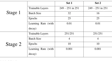
Table 7.1: Training method for YOLO experiments. Two sets, with initial batch sizes of 16 and 32 are trained. Training is done in two stages where, only the last two layers are trained in the first stage and then all layers are trained in the next stage. Batch sizes, learning rates and number of epochs were determined experimentally through trial and error. ... 33

Table 11.1: Training scheme for all experiments... 56

Table 11.2: mAP results of 32-batch version of YOLO variants on small vehicles class of DOTA dataset... 59

Table 11.3: mAP results of 32-batch version of YOLO variants on small vehicles class of DOTA dataset... 59

Table 11.4: IOU results of YOLO variants on small vehicles class of DOTA dataset. ... 60

Table 11.5: Time analysis for 16-batch models. ... 68

Table 11.6: Time analysis for 32-batch models. ... 69

Table 11.7: Results on DOTA Test Set – Top Performers. ... 70

xii

Acronyms

CNN

Convolutional Neural Network

CV

Computer Vision

FC Layer

Fully Connected Layer

FCN

1

Chapter 1

Introduction

Computer vision has made great strides over the past few decades. It is now an integral part of everyone’s lives as it is used almost everywhere, from smart phones to industrial manufacturing. Many tasks such as autonomous driving, facial recognition and optical character recognition would not be possible without computer vision. The high-level objective of computer vision is to extract information from high dimensional, real world images from which to make decisions, e.g. spotting a traffic light turn red and apply brakes to stop the car. The process of extracting such information from an image can vary. Over the past decade, deep learning methods using convolutional filters has emerged to be the leading technique for computer vision, aiding tasks such as image restoration, object recognition, pose estimation and motion estimation.

Within the field of computer vision, two chief tasks dominate research; object classification and object detection. Object classification is correctly recognizing or classifying a picture of an object. In deep learning, this is done using a neural network with c number of outputs where c is the number of objects the network has been trained on. Object detection is not only recognizing the object, but also accurately localizing it within an image. As a result, object detection is significantly more complex and is an area of intense research.

2

Fig 1.1. A typical CNN architecture for object recognition [6].

Object detection networks typically feature more than one output. Apart from the object class, they also calculate the position of objects within an image. This can be done as a separate branch within the same network or as a single stream.

3

Chapter 2

Related Work

Object detection has been the subject of much recent research due to its many applications and uses. Datasets such as MS-COCO [7] and Pascal VOC [5] have not only fueled development of data hungry methods but enabled fair comparison amongst methods.

One of the first deep networks to offer object detection was R-CNN [8] by Girshik et al. It used selective search methods to first extract regions from an image and then passed each region through an object recognition Convolution Neural Network (CNN). This was not only very slow but was also very dependent on the selective search algorithm.

Fast RCNN [9], which made use of an ROI Pooling layer on image feature maps, gave good object detection but still required an independent selective search algorithm.

Object detection drastically improved in speed with the introduction of a Region Proposal Layer in Faster RCNN [10]. This was one of the first end-to-end trainable object detection network that did not rely on an external region selection algorithm. This concept was later used in Mask RCNN [11] along with an ROI Align layer. Mask RCNN also provided methods for not only detecting objects but also labelling each pixel of the object with a class assignment.

Another, very important network to implement object detection, was You Only Look Once - YOLO [1]. YOLO initially addressed speed as its primary contribution while providing comparable detection scores. At the time it was one of the few networks to offer real time detection. Subsequent improvements to the YOLO network included YOLO v2 [3] and YOLO v3 [12]. These are elaborated in higher detail in the later sections of the document.

4 Oriented Boxes

Oriented bounding box detection is a recently introduced method that allows bounding boxes which are rotated at any angle. One of the first research methods in this area was ORN [14]. ORN uses active rotating filters which rotate while performing convolution and produce multiple feature maps with encoded rotation information. The errors from all rotated versions are aggregated to detect rotation of an object.

An implementation of R-CNN by Ni et el. [15] achieves state of the art detection on the DOTA [16] dataset. The rotation was achieved by using the region proposer layer of the R-CNN to predict bounding boxes with orientation information.

5

Chapter 3

YOLO – You Only Look Once

3.1 Background

YOLO - You Only Look Once is a deep neural network method used for object detection. It was introduced in 2012 by Joseph Redmon [1]. At the time of its release, it was the first real time network that offered high quality object detection mAP scores (63.4 on Pascal VOC 2007) [5].

Table 3.1: Comparison of object detection methods on the Pascal VOC 2007 [5] dataset as of 2015. [1]

Real Time Detectors

Detector Network Train Dataset mAP FPS 100 Hz DPM [19] 2007 16.0 100 30 Hz DPM [19] 2007 26.1 30 Fast YOLO 2007 + 2012 52.7 155

YOLO 2007 + 2012 63.4 45

Less than Real Time Detectors

Fastest DPM [20] 2007 30.4 15

Fast R-CNN [9] 2007 70 0.5

Faster R-CNN VGG-16 [10]

2007 + 2012 73.2 7

YOLO VGG-16 [1] [18]

6 It helped solved a major problem with object detection networks, which was long training and testing times. At the time, there were several state-of-the-art object detection networks such as Fast R-CNN and Faster R-CNN. However, they were far from real time, with frame rates being ~10 FPS. This made such networks ill-suited for real time object detection.

A part of the reason for this shortcoming with Fast R-CNN and Faster R-CNN was with the architecture. Images had to be passed through a feature extractor. The extracted features were then divided into regions of interest. In Fast R-CNN, the ROI selection was random while in Faster R-CNN a region proposer network was used. The regions are then regressed over to find objects in the image. This entire process, while being thorough takes a lot of time to train. The complexity also means that inference time is significantly long.

YOLO eliminated such multi-stage training, reducing learnable parameters and network complexity. By streamlining this process and reducing learnable parameters, training and inference was made faster in YOLO.

3.2 Overview of the YOLO Pipeline

There are many similarities to YOLO and YOLO 9000. The basic YOLO pipeline is discussed in this section. As with most object detection networks, YOLO also extracts feature maps from an image. This is done by a standard CNN network. The specific network used for this purpose is up to the user and can be changed as per requirement. Ideally the feature extractor must have few learnable parameters without compromising accuracy metrics.

7 The dimensions of the feature map are dependent upon the size of the input and the close clustering of objects in an image. A typical 244  244  3 input image will generate a 7  7 d number of output feature maps. The number of feature maps is d as shown in (1.1):

d = B 𝑥 5 + c (1.1)

where,

B is the maximum number of objects the network will be able to predict in each cell of the 7  7 feature map.

c is the number of classes.

8

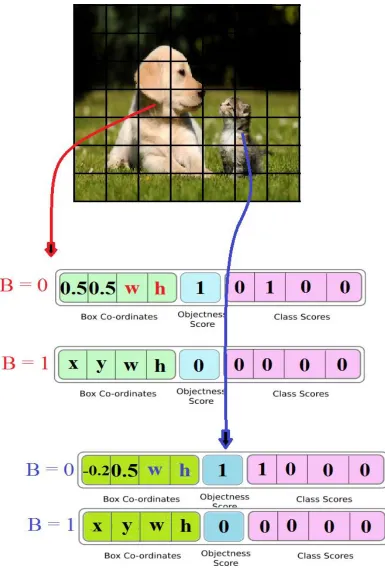
Fig 3.2 Output of YOLO network. Each box solves for 4 + 1 + C predictions for location,

objectness and class. Only the center cell in which the object centroid lies is responsible

9 In the above example a 244  244  3 images are fed into the YOLO backbone to yield a 7  7  14 feature maps. Here, B = 2 and c = 4. The network detects the presence of two objects in the whole image, one in each grid cell. As a result, the objectness for B = 0 is predicted to be ~1 for the two particular grid cells.

The x, y locations for class dog, is predicted to be 0.5, 0.5, relative to the center of that particular cell. For cat, it is predicted to be 0.2 and 0.5. The widths and heights for the two objects are also predicted as per the dimensions of the objects. InFig 1.2 the width is assumed to be w and height h.

It should be noted that the objectness for all other grid cells will be 0. Only the center grid cell of each object in the image is responsible for detection.

3.3

Non-Max Suppression

10

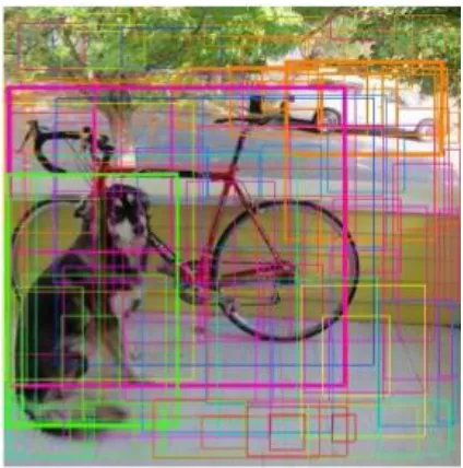
Fig 3.3. The same object is predicted thrice in this image. This could result in false positives

being counted for this image, despite the network being partially right about object location. [2] This is especially prevalent when the threshold confidence levels are set to a lower value as shown in Fig 3.4.

Fig 3.4. An example where the score threshold is set to a lower value so that more predictions

11 Such instances can be rectified by suppressing duplicate outputs or low confidence

outputs. This is done by a process called non-max suppression.

In YOLO, non-max suppression is done greedily. The bounding box with the highest confidence is firstly chosen. All bounding boxes with high IOU with this selected bounding box are discarded. Of the remaining bounding boxes, the one with the highest confidence is selected next and the process continues.

This is the last step of the YOLO detection process. The final result from YOLO on an example image is shown in Fig 3.5.

Fig 3.5. Final output of the YOLO network on an example image. [1]

3.4

Deficiencies of YOLO

12

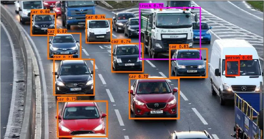
Fig 3.6 YOLO fails to detect several cars in this image. The missed detections come from objects

that are very small or very close together. It is also unable to detect same class objects of

different sizes. [21]

Since, YOLO subsamples an image using convolutions, small objects can often go undetected. YOLO is not a good classifier for extremely small objects.

13

Chapter 4

YOLO v2 – Better, Stronger, Faster

4.1

Introduction

YOLO v2 [3] and YOLO 9000 [3] are an improvement over YOLO. It has several key differences from YOLO. All of these networks work together to build a faster and more reliable network. It was introduced in CVPR 2016 by Joseph Redmon and Ali Farhadi.

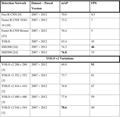
It was demonstrated to detect over 9000 object categories while providing real time detection just like its predecessor. When trained on Pascal VOC, YOLO v2 provides 76.8 mAP at 67 FPS. It gives 78.6 mAP at 40 FPS, outperforming Faster RCNN with Resnet and SSD.

14

Table 4.1 Comparison of object detection methods on the Pascal VOC 2007 + 2012 dataset as of 2015.

Detection Network Dataset – Pascal Version

mAP FPS

Fast R-CNN [9] 2007 + 2012 70.0 0.5 Faster R-CNN

VGG-16 [10]

2007 + 2012 73.2 7

Faster R-CNN Resnet [23]

2007 + 2012 76.4 5

YOLO 2007 + 2012 63.4 45

SSD300 [24] 2007 + 2012 74.3 46 SSD500 [24] 2007 + 2012 76.8 19

YOLO v2 Variations

YOLO v2 288 x 288 [3]

2007 + 2012 69.0 91

YOLO v2 352 x 352 [3]

2007 + 2012 73.7 81

YOLO v2 416 x 416 [3]

2007 + 2012 76.8 67

YOLO v2 480 x 480 [3]

2007 + 2012 77.8 59

YOLO v2 544 x 544 [3]

15

Fig 4.1 Comparison of seed and mAP scores of different object detection networks. [3]

4.2

Changes from YOLO

YOLO v2 incorporates several variations and changes over YOLO. All of these are listed below and contribute to better performance. The individual contributions of each of these is given in Table 4.2.

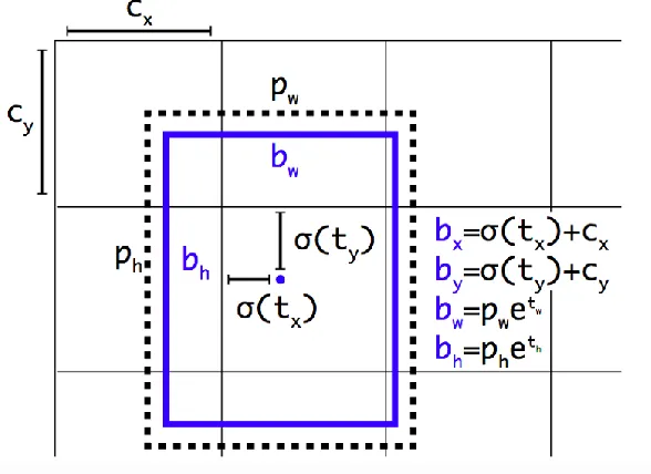
Anchor Boxes: The first improvement is the presence of anchor boxes. A set of user defined anchor boxes are taken at each grid cell. The grid cell, now has the responsibility of predicting the change in height and width of the anchor box instead of the absolute width and height. This is seen to be more robust and in line with other state of the art object detection networks such as Faster R-CNN. It also makes it easier for the network to learn box dimensions.

16 In the YOLO v2 network in Table 4.1 three anchor boxes were selected for each grid cell. If the subsamples image has 7  7 cells, there are considered to be 7 7 3 anchor boxes for that particular feature map. Each anchor box is able to predict one object.

The equation for the prediction of width and height of an object is:

𝑏𝑤 = 𝑝𝑤𝑒𝑡𝑤 (4.1)

𝑏_ℎ = 𝑝_ℎ𝑒𝑡ℎ

Where,

𝑏_𝑤is the width and 𝑏_ℎis the height. and

𝑡𝑤 and 𝑡ℎ are network predictions for width and height respectively.

The exponential function is used because of its favorable properties during backpropagation. Using an exponential function also prevents the prediction of negative values since width and height cannot be negative for an object.

Anchor Box Dimensions: While anchor box dimensions are user defined, the network is shown to benefit from picking anchor boxes that are more suited to the dataset. This is done by using K-Means clustering to pick out nine different anchor boxes.

Constrained x, y Predictions: In YOLO, the center of an object is predicted by the corresponding grid cell. The grid cell that falls in the center of the object is responsible for predicting the exact x,y location of the object box, relative to itself. In region proposal networks the coordinates are calculated as:

𝑥 = (𝑡_𝑥∗ 𝑤_𝑎) − 𝑥_𝑎 (4.2)

𝑦 = (𝑡_𝑦 ∗ ℎ_𝑎) − 𝑦_𝑎

where,

x, y are center locations of the object,

17

𝑡_𝑥 and 𝑡_𝑦 are the predictions, and

𝑥_𝑎and 𝑦_𝑎 are for the center location of the region.

By using this equation, the coordinates predicted by any one grid cell can end up in any part of the image. YOLO v2 introduces constraints on this by allowing each grid cell to predict coordinates anywhere within itself only. The center of an object predicted by a particular grid cell cannot be outside of itself. The equation now becomes:

𝑏𝑥 = σ(𝑡𝑥) + 𝑐𝑥 (4.3)

𝑏_𝑦 = 𝜎(𝑡_𝑦) + 𝑐_𝑦

Where 𝑏𝑥 and 𝑏𝑦 are the center x and y of the object.

A sigmoid operation is applied on 𝑡_𝑥 and 𝑡_𝑦, the predictions of the network. 𝑐_𝑥 and 𝑐_𝑦 is the location of that grid cell. By this equation, the center of an object cannot extend beyond the confines of the grid cell.

Fig 4.2 Object box predictions from one anchor box, belonging to one particular grid

18 High resolution Classifier: YOLO was designed to take in images that were 244  244. This made small objects very hard to recognize, especially if the image had to be resized from its original size to 244  244. YOLO v2 is trained and tested on images that are 416  416. Further, the backbone architecture is such that higher resolutions can be accepted by the network, though this will increase training and inference times.

Multi Scale Training: While YOLO did not allow training or testing with images that are of multiple scales, this is not the case with YOLO v2. Inputs can be of any dimension as long as the number of grid cells generated is odd. This allows the training to be done on multi scale images increasing robustness of the network. The network is allowed to generalize better and give higher test scores that are independent of object scale.

Darknet-19: Most object detection networks use VGG [4] as their backbone. While this is a state-of-the-art network that provides good feature extraction, there are many millions of parameters that need to be learnt. This considerably slows down the network. YOLO v2 uses Darkenet-19, a faster backbone. It has 19 convolution layers and 5 pooling layers. It mostly uses 3  3 convolutions and doubles the number of feature maps after each pooling step. Training Process: The network is first trained as an object classification network. Darknet-19 is used along with fully connected layers at the end to be trained on ImageNet 1000. Once this is done, the last fully connected layers are removed and replaced by YOLO prediction maps. This new network is then trained for detection. This process leverages the size of ImageNet training data to train more generalized filters for convolution, in the first few layers.

Hierarchical Classification: YOLO v2 is trained such that ImageNet [22] labels are pulled from WordNet [25], which is a language database that relates words to one another. For example, in [3] “Norfolk Terrier” is classified as a type of “hunting dog” which is a type of “dog”. This helps the network relate images and objects to one another.

19

20

Chapter 5

YOLO v3

5.1 YOLO v3

YOLO v3 was introduced by Joseph Redmon and Ali Farhadi in 2018 as an improvement of YOLO 9000. Just like the base YOLO network, YOLO v3 also passes the image only once through the network before making a prediction, thus retaining the “only looking once” feature of all YOLO networks. This is one of the key features which contribute to its real time nature.

The architecture can be divided into 3 parts - the backbone, the prediction feature maps, and the loss. This is especially advantageous, since it allows independent testing and modification of any one module at a time.

5.2 Overview of YOLO v3

21

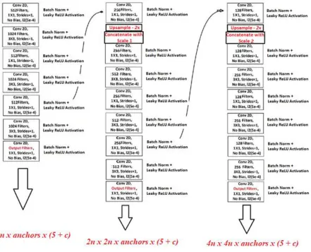
Fig 5.1 YOLO v3 backbone outputs.

Prediction feature maps - YOLO outputs set of prediction maps from an image. For example, in Fig 5.1, each one of those outputs at the different scales is a set of Bx (4 + 1 + c)

feature maps. The feature map predicts x, y locations, width, height change of anchor box along with c outputs where c is the number of classes and B is the number of anchor boxes at one scale. This helps to localize objects of different sizes.

YOLO v2 and YOLO v3 make use of anchor boxes for better prediction with tighter bounding boxes.

The backbone network partitions each feature map into ss cells. Each cell for each anchor box solves for five values: center x, y coordinates, change in w (width) and h (height) of the anchor box and objectness or confidence of an object contained within that particular cell.

If an object spans over more than one grid cell, only the center cell is responsible for detection of that particular object.

This prediction scheme is repeated for each of the three scales. Therefore, if there are 3

22 However, it should be noted that as described above, each cell can only predict threeobjects for each scale, or one object at any one anchor box aspect ratio for each scale. This is a notable shortcoming of the YOLO family. This is especially of concern when there are many objects clustered together or the objects are very small.

Losses - Because YOLO has B (5 + c)predictions at each of the ss cells, it has to have losses for all the different types of predictions. The localization loss function measures errors in the location and size of the predicted bounding box. Therefore, it is responsible for prediction of

x, y locations of the object center as well as w and h of the object:

λ

𝛴

𝛴

𝜑[(𝑥

− 𝑥̂

)

+ (𝑦

− 𝑦̂

)

] +

λ

𝛴

𝛴

𝜑 [√𝑤

− √𝑤

̂

)

+ (√ℎ

− √ℎ̂

)

]

Where,

λ

Φ = 1

λ

bounding box sizes. Smaller objects will have higher loss factor, while bigger ones have lower loss factor.

Confidence loss is expected to allow the network to detect the presence of an object. It is a measure of objectiveness. If an object is detected in the one of the ss cells, the loss for that particular cell is

𝛴

𝛴

𝜑(𝐶

− 𝐶̂

)

Where,

23 If an object is not detected, the loss becomes

λ

𝛴

𝛴

𝜑(𝐶

− 𝐶̂

)

Finally, at each cell we need to determine the likelihood of each of the c classes. The class loss is analogous to a cross-entropy loss for a classification network.

𝛴

Σ

𝜑(𝑝

(𝑐) − 𝑝̂

(𝑐))

λ

𝛴

𝛴

𝜑[(𝑥

− 𝑥̂

)

+ (𝑦

− 𝑦̂

)

] +

λ

𝛴

𝛴

𝜑 [√𝑤

− √𝑤

̂

)

+ (√ℎ

− √ℎ̂

)

] +

𝛴

𝛴

𝜑(𝐶

− 𝐶̂

) + λ

𝛴

𝛴

𝜑(𝐶

− 𝐶̂

) +

𝛴

Σ

𝜑(𝑝

(𝑐) − 𝑝̂

(𝑐))

5.3 Backbone Architecture

25

Fig 5.2. The first nine convolutions of Darknet -54. The dimensions of the feature maps

26 The output of the block in Fig 5.2is fed to the block shown in Fig 3.3.

Fig 5.3 Input from the previous block fed into 8 resblocks.

The output from this block is taken to the last few layers. This output shall be called scale 2. The input of this block would be 208208128 and the output would be 104104256.

27 This layer too serves as an important part of the last few layers. The output which would be 5252512 in our previous example shall be called scale 1.

Fig 5.5 Input from the previous block fed into 8 resblocks.

28

Fig 5.6 Input from the previous block fed into the last few convolutions to give output

prediction maps.

29

Chapter 6

Applications of YOLO

6.1 Object Detection Networks

Object detection has been a major area within computer vision research- improving mAP scores, detection times and reliability of object detection networks. As a result, several applications have been improved by incorporating computer vision.

6.1.1 Autonomous Cars

Autonomous driving is one of the most important technologies that has benefited directly because of improvement in object detection and computer vision. Several car manufacturers have already integrated some level of autonomy in their production cars. For example, Tesla cars have already incorporated lane keeping, driving assist and collision detection [26]. Waymo has also contributed greatly to this area by deploying self-driving cars for taxi’s in Phoenix, Arizona [27].

30 Several car companies have declared that they will have full autonomy by 2025 [29] [30], allowing cars to drive themselves without any user input. Such developments have only been possible because of the major strides in object detection networks. Deep learning is allowing cars to comprehend roads better, and recognize objects such as cars, trucks and pedestrians.

6.1.2 Retail

Several retailers have already made use of object detection in varying capacities. Amazon Go uses object detection to automatically charge customers for products and eliminate long checkout lines. This has been deployed at limited capacity at Seattle [31]. By detecting products and automatically noticing their presence or absence, retailers can use object detection networks to detect item theft and stock inventory.

6.1.3 Aerial Imaging

There are several applications within aerial imaging that can be simplified using object detection. In security and surveillance, detection of vehicles and humans can be used to aid law enforcement and improve tracking of objects of interest. Many companies have also invested in deep learning to assist agriculture and resource detection. Ceres Imaging is one such company that uses aerial imaging to detect agricultural yield and resource management. Improvements in high resolution satellite imagery and drone imaging have introduced new avenues to explore.

6.2 YOLO in Aerial Imaging

YOLO is an excellent network that is well suited for aerial object detection. This is partly because of the real time nature which allows fast moving objects to be easily detected and tracked. This is especially useful in applications such as missile technology and police surveillance of suspects.

31

6.3 Shortcomings of YOLO

All three version of YOLO address one of the most important issues with deep learning for object detection- timing. YOLO is an excellent network for applications that demand real time detection such as aerial imagery.

However, there are several shortcomings of YOLO that need to be addressed. These shortcomings prevent or hinder several applications within aerial imaging and need more research. 1. Tightness of boxes – Despite being an excellent network in terms of speed and detection accuracy, YOLO does not give box detection that are as accurate or tight as several other state of the art networks such as Mask R-CNN [11] or Faster R-CNN [10]. This could be problematic when objects are close together and tracking is necessary.

2. Overlapping objects – Because of the YOLO architectures, they are limited in how many objects they can detect within one grid cell. Depending on how the network is designed, YOLO v3 can detect up to BS objects in each grid cell where B is the number of anchors in each cell and S is the number of scales.

32

Chapter 7

Oriented Bounding Boxes

Native YOLO v3 falls short in providing tightness of bounding boxes when objects are placed orthogonally. This is detrimental to computer vision. In this thesis, we explore ways in which YOLO v3 can be modified to provide better bounding boxes for objects without compromising on mAP scores. We explore several methods to provide such oriented bounding boxes and compare them to each other, laying a baseline for future research. To verify results and visualize them, experiments are conducted on the DOTA dataset [15].

7.1

Experiment Methodology

Changes to YOLO v3 are done in stages in order of simplicity. The entire process can be divided into three subprocesses:

1. Allowing anchor boxes to rotate.

2. Adding extra anchor boxes while restricting rotation.

3. Changing YOLO v3 to predict four points instead of center, height and width.

All experiments are carried out using Keras with Tensorflow back-end. The methodology for each of the subprocesses mentioned above are specified in higher detail in the next few chapters. Each of the resulting networks are trained and tested on the DOTA large scale aerial dataset.

33

Table 7.1 Training method for YOLO experiments. Two sets, with initial batch sizes of 16

and 32 are trained. Training is done in two stages where, only the last two layers are trained in

the first stage and then all layers are trained in the next stage. Batch sizes, learning rates and

number of epochs were determined experimentally through trial and error.

Stage 1

Set 1 Set 2 Trainable Layers 249 – 251 in 251 249 – 251 in 251

Batch Size 32 16

Epochs 25 25

Learning Rate (with decay)

0.01 0.01

Stage 2

Trainable Layers 251/251 251/251

Batch Size 4 4

Epochs 10 10

Learning Rate (with decay)

0.001 0.001

7.2 DOTA Dataset

34

7.3 Dataset Preprocessing

Since YOLO is agnostic to image size, the architecture itself does not oppose the wide variations in aspect ratio or image size. However, using such images reduces the relative size of objects within the image, making it harder for the network to learn. Hence, the images are cropped to 1024  1024 chunks from large and unbalanced sizes of ~ 3000  1000. This is done by using a sliding window approach recommended by [15]. Cropping ensures that the images are all of equal sizes and aspect ratio. The number of images is also expanded to 30628.

35

Fig 7.1 Two crops, image 1 and image 2 of size 1024  1024 being extracted from an

36

7.4 Incorporating Angle to Annotations

Be default the dataset does not include angle. We calculate angle at the time of preparing the dataset, to be fed into the network.

As shown in Fig 7.2, all possible rotations of an object can be covered by rotations of 45 degrees around each axis. This is possible because we do not discriminate between the front and rear of an object, therefore an object that is rotated by 180 is taken to be the same as one that is at 0 degrees.

Fig 7.2. All possible rotations of an object. The mirror image of each of these objects

37 To calculate the angle of rotation of each object, we measure the angles of inclination of two adjacent sides of the object. We always measure the angle of inclination of an object from the x-axis. Since the objects are rectangular, one of the angles of inclination must be less than or equal to 45 degrees. This is shown in Fig 7.3 where the object orientation increases from 0 degrees to 45 degrees. In the last tile, the object inclination increases further to 80 degrees, however by the algorithm, we take this inclination to be –10 degrees instead. This is to reduce the amount of rotation required to be predicted by the network. We try to keep the degree of rotation as small as possible to put less strain on the learning process of the network.

We find this method to be efficient and reliable in most cases. By using this method both training and testing of the network is simplified. Visualization is also more intuitive and better written using this method.

38

Fig 7.3. The object rotation starts at 10 degrees from the x axis and then increases to 45 degrees.

In the last tile, the object is rotated further along to 80 degrees, however, we calculate this to be

-10 degrees to encourage small angles of rotation.

39

Fig 7.4. Such errors in annotation are approximated by the algorithm. Here the rotation of the

object is approximated to 45 degrees. In this figure, the object is drawn by the black lines and

40

Chapter 8

Rotating Anchor Boxes

8.1 Introducing Rotation

While there have been papers that have implemented rotated predictions for objects, none of them have incorporated these rotations for YOLO v3 or any other real time network. The first method of implementing rotation is to allow the rotation of the anchor boxes themselves. In YOLO v3 and YOLO v2, the anchor boxes had the freedom to morph their height and width to suit the object being predicted. Similarly, we introduce the ability to morph angle as well.

8.2 Rotated Anchor Boxes

41

Fig 8.1 Predictions for a grid cell from the YOLO – Rotated network. The values in the blue

boxes are for x, y, width and height. Alongside, we also predict angle, objectness and class.

8.3 Activation of Angle

A sigmoid was used for the activation of x, y coordinates and an exponential function was used for width and height. The activation function for angle must be differentiable, linear in the range of freedom of movement in degrees and preferably predefined in Keras. One of the steps taken in the process is to visualize the box as being centered at 0 degrees and then allowed to ‘wiggle’ a certain amount clockwise and counterclockwise. The total wiggle area is its freedom of movement. The angle activation function used is

Ө = 𝑤𝑖𝑔𝑔𝑙𝑒 𝑥 (𝜎(𝑝𝑟𝑒𝑑) −1

2) (8.1)

The output of the network is run through a sigmoid activation to scale it from 0 to 1. It is shifted by half, to change the scaling to -0.5 to 0.5. To visualize the allowable bounding box, the total wiggle amount in degrees is multiplied so that the wiggle of the box becomes − 𝑤𝑖𝑔𝑔𝑙𝑒

42

𝑤𝑖𝑔𝑔𝑙𝑒

2 degrees. This is shown in Fig 8.2 and 8.3 where all anchor boxes for a scale are centered

around their axes but have the freedom to wiggle a certain amount around zero.

Fig 8.2 Top shows a box centered at its axis. The two figures below, show its wiggle of +/- ten

43

Fig 8.3 The box is overlaid with its wiggle.

8.4 Angle Loss

We experimented with two different types of losses for angle, cross entropy as well as square loss. In both cases, the angle was scaled from 0 to 1. For example, if a box was given the freedom to rotate between -10 degrees to 10 degrees, it would be scaled from 0 to 1 before feeding to the loss function.

For cross entropy loss, we divided the angle levels from 0 to 1 into 10 buckets. It was expected that this would be easier to learn with a tradeoff in accuracy of angle.

Square loss was simply a square of the difference between scaled values of prediction and ground truth as shown in equation below.

𝐴𝑛𝑔𝑙𝑒 𝑙𝑜𝑠𝑠 = (𝑃𝑟𝑒𝑑𝑖𝑐𝑡𝑒𝑑 𝐴𝑛𝑔𝑙𝑒 − 𝐺𝑟𝑜𝑢𝑛𝑑 𝑇𝑟𝑢𝑡ℎ 𝐴𝑛𝑔𝑙𝑒)2 _(8.2)

8.5 IOU of Boxes

Adding an angle parameter to a bounding box, introduces additional complexity for calculating IOU. Without angle, the IOU is calculated by (8.3) and shown in Fig. 8.4.

𝐼𝑂𝑈 =

44

Fig 8.4 Pictorial representation of intersection and union of two boxes, B1 and B2 [4].

By including angle, we can no longer use this method of calculating IOU. We calculate the new IOU by first treating it as if it were not rotated at all. We first use (8.2) to calculate its IOU, then we multiply this by an angle IOU factor, that is defines in (8.3).

𝑎𝑛𝑔𝑙𝑒 𝐼𝑂𝑈 𝑓𝑎𝑐𝑡𝑜𝑟 = 1 −

𝑤𝑖𝑔𝑔𝑙𝑒

2

(

45 Fig 8.5 Change in angle IOU factor with respect to change in angle for a wiggle of 1 degree.

8.6 Evaluating the model

46

Chapter 9

Rotations with Extra Anchor Boxes

9.1 Anchor Box and Wiggle Tradeoff

While increasing wiggle for anchor boxes will allow them to accommodate greater variations of objects, it can come at a price. Increasing this wiggle means that there will be a greater range of angles for it to learn. Further, the greater the wiggle, the increased difficulty in predicting the ground truth angle. For these reasons, it is worth exploring the idea of adding more anchor boxes, centered at various angles, while reducing wiggle in each of the boxes.

We set up a baseline for adding anchor boxes and experiment with changes in IOU and mAP scores for the same dataset.

9.2

Adding Anchor Boxes

The previous version of the network, as well as both YOLO v3 and YOLO v2 had three anchor boxes per scale. We take this further by doubling the number of anchor boxes and going from three to six anchor boxes per scale. In addition to the previous boxes, we also add boxes of the same height and width, at an offset of 45 degrees. This is shown in Fig 9.1.

Fig 9.1. On the left, in red are the three anchor boxes that were originally present in YOLO. To

the right, in blue are the three anchor boxes that we have added. As shown, the new anchor boxes

47

9.3 Wiggle for Anchor Boxes

Since, we have more anchor boxes covering each grid cell, we can restrict the wiggles of each anchor box to 45 degrees, or 22.5 degrees to either side of their center. This is the minimum wiggle angle at which objects at all rotations can be covered. Increasing the wiggle beyond this, will only cause the boxes to predict identical ground truth objects, giving us no added advantage. At the same time, reducing the wiggle prevents objects at higher rotation angles from being detected. Fig 9.2 shows the six anchor boxes along with their freedom of rotation about their axes.

Fig 9.2. The six anchor boxes used by this variation of the YOLO network. The center boxes are

48

9.4 Training Specifications

49

Chapter 10

Deformable Anchor Boxes

10.1

Shortcomings of Rotated Anchor Boxes

While rotated anchor boxes are a simple solution to an important problem, it is limited by the rectangular shape that it can predict. It is desirable to additionally predict non-rectangular shapes like trapezoids, rhombus, and parallelograms. To remedy this problem, we propose using deformable anchor boxes as an alternate form of incorporating orientation. In this variation of the YOLO, the network is free to move the four bounding box corner points to anywhere within the image, allowing predictions for irregular as well as regular shapes.

As in the previous network, we opted for six anchor boxes per scale to keep displacements low and ensure that objects of all orientations and alignments are detected.

10.2 Selection of Anchor Box

50

Fig 10.1. The box in blue is the anchor box for which distance is measured from the corresponding point.

We have four cases as shown, where the lines in red represent distances measure from the corresponding

point. The sum of all these distances are taken for each case. The case that gives the minimum sum of

distances will be selected as the optimum configuration. We use this process to select the best anchor box

as well. In this figure, the case on the top left will give the least sum of distances.

We repeat this for all anchor boxes in the scale and assign the anchor box that gives minimum value to that object. While this does not calculate the IOU of the object and the anchor, it is reliable at selecting the best anchor for an object.

10.3 Activation Function for Point Values

51 point from its point of origin. For this we cannot use a sigmoid or an exponential as was used in prediction of x, y, dimensions or angle. The reasons being:

1. A sigmoid and exponential function output values between 0 and 1. It is possible that the point can be moved in the opposite or negative direction, which cannot be accommodated by sigmoid.

2. The above issue could be solved if we were to scale the entire image from 0 to 1 so as to allow a point to move anywhere in the image. However, by nature of the activation function we need the network to be encouraged to make predictions that are close to the anchor point initial estimates.

3. A sigmoid would give equal tendency for the network to predict the point anywhere within the image.

4. An exponential would be an even more dangerous choice, because it would prevent prediction of points that are too far away from the initial estimate in the positive direction while making no such restrictions in the other direction.

In choosing a good activation, the motivations were: 1. The function must be differentiable.

2. The function and its inverse must be defined at all points in the coordinate plane.

3. The function must try to push the network to predict minimal displacement from the starting points so that the anchor points do not end up too far away, within the image. 4. Ideally, it must be intuitive.

We find sinh activation, to satisfy all requirements. It mimics the exponential curve on both halves of the coordinate plane and allows for movement in both directions of the axis.

52

Fig 10.2. The activation function, sinh(x/3) used to predict the displacement of anchor points.

53

Fig 10.3 arcsinh(x), showing its good curve and gradient.

10.4 Calculating IOU

We use the same process as given in Section 10.2 to pick the best IOU. Since, we cannot calculate IOU directly from this process we use an approximation algorithm as given in (10.1).

𝐼𝑂𝑈

=

4 𝑖=1 )

54 We take the sum of all corresponding point distances 𝑑_𝑖 between predicted point and ground truth box corresponding point. We subtract this from the length of the diagonal of the ground truth 𝑑𝑖𝑎𝑔_𝐺.𝑇. This is scaled to one by dividing by the length of the ground truth diagonal.

We threshold this by 0.5. Anything that is equal to or higher than 0.5 is taken to be a match while anything that is lesser is discarded.

While this is not an optimum method of calculating IOU, it is logically sound and serves its purpose well, in determining if an object has been correctly predicted by the network.

10.5 Loss Function for Deformable Point Network

The loss function for this network includes eight different losses for all of the point predictions. Each point prediction has two losses for x displacement prediction and y displacement prediction.

For the loss function we use the standard square loss as shown in (10.2) and (10.3).

𝑥 𝑑𝑖𝑠𝑝𝑙𝑎𝑐𝑒𝑚𝑒𝑛𝑡 𝑙𝑜𝑠𝑠 = (𝑃𝑟𝑒𝑑𝑖𝑐𝑡𝑒𝑑 𝑥_{𝑑𝑖𝑠𝑝𝑙𝑎𝑐𝑒𝑚𝑒𝑛𝑡}− 𝐺𝑟𝑜𝑢𝑛𝑑 𝑇𝑟𝑢𝑡ℎ 𝑥_{𝑑𝑖𝑠𝑝𝑙𝑎𝑐𝑒𝑚𝑒𝑛𝑡})2 _(10.2)

55

Chapter 11

Experiment Design

11.1 Motivation and Objective

The prime concern when designing experiments was to proceed by making small changes to the network and learning from each individual modification. In the interest of ease and simplicity, we tried to divide experiments into smaller sub-experiments. We first restricted all experiments to only one single class of the DOTA dataset, which was small vehicles. This gave us a training set of about 3300 images and a test set of 600 images.

The issues that we were trying to address were:

1. How does rotation affect network performance?

2. Would the addition of anchor boxes while consequently restricting rotation have any benefits?

3. Will the ability to deform a box shape have any effect on network performance and if so in what way?

Finally, we also wanted to set a precedent for other researchers to carry forward this work.

11.2 Training Scheme

As mentioned earlier, we started with a pretrained version of YOLO v3 for all our

experiments. The network was pretrained on MS-COCO using Darknet–54. We used a two-stage scheme, as shown in Table 5.1 for our experiments. We first trained the last two layers of the network for 25 epochs. We then pick the best model from these 25 epochs and then train that model for another 15 epochs. During this second phase of training, we unfreeze all layers and train the whole network.

56

Table 11.1 Training scheme for all experiments.

Training Scheme

Trained

Layers Epochs

Dataset

Size Batch Size

Learning

Rate Decay Patience

Take Best

in All

Epochs

Last 2

Layers 25 3463

Can

Change 0.01 0.3 3 YES

All Layers 15 3463 4 0.001 0.3 3 YES

As shown in Table 11.1, we used a learning rate decay scheme, where the learning rate was reduced by a factor of 3 when the validation loss remained unchanged for three epochs.

11.3 Testing

Testing was done on a held-out test set of 600 images. We ran the evaluation script given by [15]. We also evaluated each network for the average IOU for all detected objects. Since only predictions with an IOU of greater than 0.5 are considered to be valid, the average was always higher than this.

We also evaluate the time taken by each of these networks so that future researchers may be able to extend their studies by augmenting the data taken from these experiments. This also allows users to make an educated decision on which network to use for their object detection applications.

10.4 Training – Getting Started

We have included the code for all variants of YOLO in //github.com/axb4012/keras-yolo3. We have tried to keep the training as user friendly as possible. The user is only required to change paths in constants.py. The steps for training are as follows:

1. Change train path – This is the location of the training annotation files.

57 3. Change batch size – While the batch size for the second stage is kept constant at 4, the

initial batch size can be changed to user preference.

4. Run train.py – The input command to train would be python

11.4 Experiments with Angle

To help gain insight in how well the networks were working, we created four train and test sets: 1. Set containing objects rotated from their axes by 10 degrees to either side. We shall

call this 10-degree set.

2. Set containing objects rotated from their axes by 25 degrees to either side. We shall call this 25-degree set.

3. Set containing objects rotated from their axes by 45 degrees to either side. We shall call this 45-degree set.

4. Set containing all objects, irrespective of rotation.

It should be noted that even though, theoretically the 45-degree set must encompass all objects, it does not because of artifacts in annotation as described in the later sections.

11.5 Experiments with YOLO v3

We test YOLO v3 on all four sets. Additionally, we also present results for non-oriented experiments on YOLO v3. This is so that we set a baseline result on YOLO v3. By this experiment we take the minimum x, y and maximum x, y coordinated of the ground truth points as object labels.

11.6 Experiments on YOLO Rotated

We train three variants of the YOLO Rotated network:

1. Anchor boxes only allowed to rotate by 10 degrees to either side of the network. We shall call this 10-degree network.

58 3. Anchor boxes only allowed to rotate by 45 degrees to either side of the network. We shall

call this 45-degree network.

All three variants of the network are tested on all four test sets. We present results and conclusions in the next sections.

11.7 Experiments on YOLO Extra Anchors

We test the YOLO Extra Anchors network on all four datasets and present results in the next chapter. All hyperparameters remain unchanged. The freedom of rotation or wiggle to each side from axis is 22.5 degrees.

11.8 Experiments on Deformable YOLO

Just like YOLO Extra Anchors, we test Deformable YOLO on all four-test set and present results in the coming sections.

11.9 Results of Experiments

59

Table 11.2 mAP results of 16-batch version of YOLO variants on small vehicles class of DOTA

dataset.

Network Test Set

YOLO Variant 10 Degree Only 25 Degree Only 45 Degree Only All

YOLO v3(oriented) 16.45 27.78 30.71 43.93

YOLO v3 18.8 32.5 52.61 68.27

YOLO v3 - 10 21.9 18.36 15.69 29.5

YOLO v3 - 25 26.43 32.93 24.8 31.14

YOLO v3 - 45 18.59 33.4 46.94 55.89

YOLO v3 EA 17.03 25.9 47.44 59.1

Deformable YOLO 16.97 25.04 24.28 41.62

Table 11.3 mAP results of 23-batch version of YOLO variants on small vehicles class of DOTA

dataset.

Network Test Set

YOLO Variant 10 Degree Only 25 Degree Only 45 Degree Only All

YOLO v3(oriented) 15.78 17.95 17.41 30.09

YOLO v3 19.07 27.68 52.5 67.28

YOLO v3 - 10 21.94 18.13 14.85 21.15

YOLO v3 - 25 26.76 35.96 27.21 36.44

YOLO v3 - 45 18.54 26.74 40.92 47.18

YOLO v3 EA 14.83 27.95 43.16 58.89

Deformable YOLO 14.58 20.51 38.6 47.93

60

Table 11.4 IOU results of YOLO variants on small vehicles class of DOTA dataset.

Network Test Set

YOLO Variant 10 Degree Only 25 Degree Only 45 Degree Only All

YOLO v3(oriented) 0.69 0.66 0.63 0.67

YOLO v3 0.67 0.66 0.66 0.66

YOLO v3 - 10 0.71 0.7 0.7 0.71

YOLO v3 - 25 0.72 0.72 0.71 0.72

YOLO v3 - 45 0.71 0.71 0.7 0.7

YOLO v3 EA 0.69 0.66 0.63 0.67

Deformable YOLO 0.68 0.68 0.65 0.67

11.10 YOLO v3

The results for YOLO v3 are presented as a baseline. We present both oriented and non-oriented results for YOLO v3. The low scores for YOLO v3 in 11.2 and 11.3, seen in the first row, on the oriented test, shows that there is much room for improvement and highlights the deficiency of the network when it comes to oriented detections. It should be noted that the strength of YOLO is in its speed while providing good mAP scores.

Further, on the oriented set, YOLO offers low mAP and IOU (Table 11.4, row 1), indicating that the boxes are not tight. This is addressed by our networks. The visualization in Fig 11.1 confirms this. While cars that are at 0 degree from their axes are detected accurately, slanted cars, are detected by boxes with low IOU.

61

Fig 11.1 Detection visualization for YOLO v3, without any rotation. The pink box and

circles are detections while blue circles are ground truth.

11.11 YOLO Rotated

10 - degree

62

Fig 11.2 Detection visualization for YOLO v3, with +/- 10-degree rotation. The pink

boxes are detections while blue circles are ground truth. Note the mistaken identifications which

contributed to low scores.

25 - degree

63

Fig 11.3 Detection visualization for YOLO v3, with +/- 25-degree rotation. The pink

boxes are detections while blue circles are ground truth. The network detects objects that are

rotated by almost +/- 25 degrees, giving false predictions.

45 – degree

64

Fig 11.4 Detection visualization for YOLO v3, with +/- 45-degree rotation. The pink

boxes are detections while blue circles are ground truth. The network detects large vehicles as

small vehicles which leads to lower scores

From running the freedom of rotation tests, we can conclude that the network demonstrates a clear ability to learn orientation. Just like YOLO, this is done in one single step and therefore does not compromise on time constraints. Most importantly, it is evident that the network obeys rotation constraints set upon it and behaves as predicted. From these results we can also come to the conclusion that each variant performs best on the angle that it was trained on.

65

11.12 YOLO – Extra Anchors

Our intuition of adding more anchor boxes while restricting rotation, clearly produces positive results. Table 11.2 and 11.3, row 6 show that mAP scores on the entire dataset improves by about 4% on the 16-batch set and 11% on the 32-batch set, when compared to the 45 – degree model on the row 5 of both tables. This is a clear indication of the robustness of the model as well as the concept of restricted rotation while adding extra anchor boxes. We can see that the best network offers a mAP score 59.1 % as compared to a non-oriented score of 68.2 %. Such a drop is to be expected as the network has more parameters to learn and is also a more complicated architecture.

66

Fig 11.5 Detection visualization for YOLO v3 Extra Anchors. The pink boxes are

detections while blue circles are ground truth. The network accurately detects objects of all

rotations.

11.13 Deformable YOLO

67 11.5, row 7 that the IOU is 0.67, which is comparable with YOLO Extra Anchors. The visualizations in Fig 11.3 provide better information about the model, since we see that the boxes predicted are deformable. They can change to irregular four-point shapes and are not restricted like our previous models. We can conclude that the best deformable model, which is the 32-batch model gives a mAP score of 47.93% is only beaten by the Extra Anchors model which has a mAP score of 58.89%.

Fig 11.6 Detection visualization for Deformable YOLO. The pink boxes are detections

while blue circles are ground truth. The network predictions are not restricted to rectangles or

68

11.14 Time Sensitivity

One of the best features of YOLO is its time sensitivity. Our models are the first to incorporate rotation and deformable points into YOLO.

We trained our models on a 12 core Intel Xeon CPU E5-2650 v4. The 16-batch models were trained on an NVIDIA Tesla M40 with 24 GB of memory. The 32-batch models were trained on an NVIDIA V100 with 32 GB of memory. The 16-batch models took about 12 hours to train on a subset of the DOTA dataset size which had 3300 images of 832 × 832. The 32-batch models took around 7 hours to train on the same dataset.

For testing, we used an Intel Xeon CPU E5-2623 with 4 cores and an NVIDIA Tesla P100 GPU with 12 GB of memory. We have listed our testing times in Table 11.5 and 11.6.

As of February 2019, ours is the only model that offers angle or deformity in predictions at speeds comparable to YOLO v3.

Table 11.5 Time analysis for 16-batch models.

Network FPS

YOLO v3 9.931

YOLO v3 - 10 9.686

YOLO v3 - 25 10.355

YOLO v3 - 45 10.706

YOLO v3 Extra Anchors 9.638

69

Table 11.6 Time analysis for 32-batch models.

Network FPS

YOLO v3 10.17

YOLO v3 - 10 10.518

YOLO v3 - 25 9.971

YOLO v3 - 45 10.625

YOLO v3 Extra Anchors 9.724

Deformable YOLO v3 9.3

We find that there is only marginal drop in FPS between YOLO v3 and deformable YOLO. The greatest drop was 8.5% from YOLO v3 benchmarks. This is acceptable and will not compromise the real time nature of YOLO. All other drops were even lesser.

11.15 Results on Official Test Set

We ran a trained version of rotated YOLO with extra anchor boxes on the official test set from DOTA. A few points to note are:

1. A lot of the results used extensive hyperparameter optimization and trained on several scales of the dataset. We did not do this since this would introduce complications on NMS and training time.

2. Many of the results on the leaderboard used ensembles of models trained on each object class. Once again, this would have meant enormous GPU and manpower resources. Since the objective of the thesis was to develop a fast variation of YOLO v3 that could