Recent and future developments in earthquake ground
motion estimation
John Douglasa,∗, Benjamin Edwardsb
a
Department of Civil and Environmental Engineering; University of Strathclyde; James Weir Building; 75 Montrose Street; Glasgow; G1 1XJ; United Kingdom
b
Department of Earth, Ocean and Ecological Sciences; School of Environmental Sciences; University of Liverpool; Jane Herdman Building; Liverpool; L69 3GP; United Kingdom
Abstract
Seismic hazard analyses (SHA) are routinely carried out around the world
to understand the hazard, and consequently the risk, posed by earthquake
activity. Whether single scenario, deterministic analyses, or state-of-the art
probabilistic approaches, considering all possible events, a founding pillar
of SHA is the estimation of the ground-shaking field from potential future
earthquakes. Early models accounted for simple observations, such that
ground shaking from larger earthquakes is stronger and that ground
mo-tion tends to attenuate rapidly away from the earthquake source. The first
ground motion prediction equations (GMPEs) were, therefore, developed
with as few as two principal predictor variables: magnitude and distance.
Despite the significant growth of computer power over the last few decades,
and with it the possibility to compute kinematic or dynamic rupture models
coupled with simulations of 3D wave propagation, the simple parametric
GMPE has remained the tool of choice for hazard analysts. There are
nu-merous reasons for this. First and foremost GMPEs are robust and reliable
∗Corresponding author
Email addresses: [email protected](John Douglas),
within the model space considered during their derivation, and many can be
extrapolated to a degree beyond this space with some confidence. With ever
expanding datasets and improved metadata the models are becoming more
and more useful: a range of predictor variables are now used, describing
the source, path and site effects in detail. GMPEs are also relatively easy
to implement and computationally inexpensive. Despite this, probabilistic
hazard calculations using GMPEs and accounting for uncertainties can still
take several days to run. Full simulation-based approaches, therefore, clearly
lie outside the computation budget afforded to most projects.
As well as the ever expanding list of predictor variables, other recent
de-velopments have also significantly improved the predictive power of GMPEs.
This has allowed them to maintain their advantage over more ‘physical’
sim-ulation techniques. Possibly the biggest aspect of this is not related to the
median ground-shaking field, but rather its variability (and correlation in
space and with oscillator period). This is a major advantage of empirical as
opposed to simulation approaches, which typically struggle to replicate the
covariance of input variables and, consequently, the variance of the ground
motion. In this article we summarize some of the recent advances in ground
motion prediction equations, including their application in SHA. We begin
with a summary of the current state-of-the-art, then introduce the main
ad-ditional predictor variables now used. Region- and event-type (tectonic or
induced) specific predictions and adjustments are then discussed. Additional
topics include advances in estimating ground-motion variability (epistemic
and aleatory) and expanding GMPEs to predict other intensity measures
or waveform features. The article concludes with a discussion on the path
forward in earthquake ground motion prediction.
seismicity, seismic hazard, ground-motion model
1. Introduction
1
Seismic hazard assessment for a given site is founded on two pillars:
2
firstly, a seismic-source model quantitatively describing all possible
earth-3
quakes in the vicinity (generally within about 300 km) and, secondly, a
4
ground-motion model expressing the shaking that would happen at the site
5
given the occurrence of each of these earthquakes. This article focuses on the
6
second of these components; nevertheless, when considering ground-motion
7
models it is vital to bear in mind the descriptions of earthquakes contained
8
within the seismic-source model. These descriptions invariably consist of
9
the earthquake’s geographical location (and depth), its magnitude and,
in-10
creasingly, its faulting mechanism and other characteristics (e.g. rupture
11
geometry).
12
The results of seismic hazard assessments are vital inputs to earthquake
13
engineering as they provide the motions that need to be resisted by
struc-14
tures and infrastructure constructed at the site. In the past most earthquake
15
engineering analyses were based on the response spectral representation of
16
shaking (e.g. Newmark and Hall, 1982; Chopra, 1995) or other
pseudo-17
static methods. Consequently only estimates of scalar intensity measures
18
(IMs), the principal ones being peak ground acceleration (PGA) and velocity
19
(PGV) and elastic response spectral accelerations (SA) at various structural
20
periods between 0 and commonly 2 s, were required for engineering
analy-21
sis. In the past decade or so, Incremental Dynamic Analysis (Vamvatsikos
22
and Cornell, 2002) and other time-history-based approaches have become
23
increasingly used. There is a growing need, therefore, for seismic hazard
analysts to provide a time-history representation of earthquake shaking in
25
addition to estimates of various IMs.
26
As stated by Douglas et al. (2015), although the characterization of
27
earthquake shaking by a single number (an IM) is a great simplification,
28
it makes seismic hazard assessment much more straightforward since the
29
link between the seismic-source and ground-motion models can be expressed
30
as a closed-form equation [ground motion prediction equations (GMPEs),
31
also known as attenuation relation(ship)s] to estimate the probability of
32
exceeding a given level of earthquake shaking. These probabilities are
cal-33
culated through probabilistic seismic hazard assessment (PSHA) (Cornell,
34
1968; McGuire, 1976), which is the basis of most current seismic design maps,
35
e.g. the National Annexes of Eurocode 8 (Comit´e Europ´een de
Normalisa-36
tion, 2005) and ASCE-7 (ASCE, 2013). Consequently it is still common to
37
assess seismic hazard using PSHA through ground-motion models that
re-38
turn IMs. Then, based on this analysis and if needed, to obtain earthquake
39
time-histories for the most important scenarios, generally defined using
dis-40
aggregation (Bazzurro and Cornell, 1999), either through selection from a
41
databank of natural accelerograms (NIST, 2011) or simulations of artificial
42
records (Douglas and Aochi, 2008).
43
Because of the key role they still play in seismic hazard assessment, this
44
review focuses on GMPEs derived empirically (i.e. from seismograms of real
45
earthquakes). The purpose of this article is not to repeat the historical
re-46
view of empirical ground motion estimation presented by Douglas (2003a)
47
nor the overall scope of the review of all methods for ground-motion
pre-48
diction by Douglas and Aochi (2008). Rather, this article seeks to review
49
the great advances in ground-motion prediction over the past decade and to
50
provide the reader with an overview of the principal topics of research. The
article concludes with some recommendations for future developments.
52
Although much of the following discussion concerns topics that are
rel-53
evant for all tectonic regimes (e.g. shallow active crustal, subduction and
54
stable continental) the examples are mainly taken from studies related to
55
ground motions in shallow active crustal environments. A review focused
56
on other tectonic regimes may emphasize other issues (e.g. the importance
57
of focal depth for subduction events and simulation-based ground-motion
58
models for stable continental regions). The wealth of data from shallow
59
active crustal areas means that epistemic uncertainties are probably lower
60
than in other tectonic regimes (e.g. Douglas, 2010b, Compare Figures 2, 8
61
and 10). For instance, in some tectonic regimes (e.g. oceanic crust, deep
62
Vrancea-type and the Himalaya) there are few strong-motion observations to
63
constrain ground-motion models and consequently the epistemic uncertainty
64
for these regions is much higher than for shallow active crustal areas.
65
2. Summary of current state of practice
66
It has now been more than fifty years since the first ground-motion model
67
accounting for both magnitude and distance dependence was derived
(Es-68
teva and Rosenblueth, 1964). Models are currently published at the rate of
69
more than one per month and, at the last count, the total number of
empir-70
ical equations for the prediction of PGA was 400 with many more based on
71
simulations (Douglas, 2016). The close match between the rate of increase
72
in strong-motion recordings and the number of GMPEs is shown in Figure 1.
73
The rapidly increasing number of GMPEs led Bommer et al. (2010) to
rec-74
ommend criteria for the selection of GMPEs to retain only those models for
75
consideration that could be thought of as representing the state of the art.
1970 1975 1980 1985 1990 1995 2000 2005 2010
Number of records
0 1000 2000 3000 4000 5000 6000
All
Mw≥ 5 & Repi≤ 200km
Date
1970 1975 1980 1985 1990 1995 2000 2005 2010
Number of GMPEs
[image:6.595.132.465.132.380.2]0 20 40 60 80 100 120
Figure 1: Available strong-motion records from RESORCE (Akkar et al., 2014b) (left-hand
axis) and number of published GMPEs from Douglas (2016) (right-hand axis) against date
for Europe and the Middle East (up to 2012).
They also suggest that these criteria could be used as a quality assurance
77
step to guide publication of new GMPEs.
78
A brief comparison between the first ground-motion model (Esteva and
79
Rosenblueth, 1964) and the recently-published GMPE of Abrahamson et al.
80
(2014) helps demonstrate the developments in this field. The GMPE of
81
Esteva and Rosenblueth (1964) was based on only 46 records and its three
82
coefficients were estimated via standard least-squares regression. In contrast
83
the model of Abrahamson et al. (2014) is based on over 15 000 records from
84
more than 300 earthquakes and its roughly 40 coefficients were determined
85
based on random-effects regression (Abrahamson and Youngs, 1992) or
strained based on ground-motion simulations or physical reasoning. Little
87
information is provided on the data behind the model of Esteva and
Rosen-88
blueth (1964) and it is thought that these data were obtained from various
89
sources with seemingly little regard to their consistency or validity. In
con-90
trast, the model of Abrahamson et al. (2014) is the outcome of careful data
91
collection via the NGA projects (Power et al., 2008; Bozorgnia et al., 2014).
92
The GMPE of Esteva and Rosenblueth (1964) is only for PGA and PGV
93
because before the Caltech Blue Books (Brady et al., 1973) response
spec-94
tra were difficult to obtain; whereas the model of Abrahamson et al. (2014)
95
provides predictions for PGA, PGV and pseudo-SA at 22 periods between
96
0.01 and 10 s. Finally, as is common for early GMPEs, Esteva and
Rosen-97
blueth (1964) do not report the standard deviation (σ) of their equation;
98
whereas Abrahamson et al. (2014) concentrate much of their effort on
de-99
riving a complexσ that models the different components of ground-motion
100
variability.
101
In the decade or so since the review by Douglas (2003a) GMPE
devel-102
opers have concentrated on: improvements in the estimation of the
ground-103
motion variability associated with their models and its components (see
104
Section 5); a move away from simple regression-based curve fitting;
at-105
tempts at using non-parametric techniques; the use of much more and higher
106
quality data; attempts at including additional independent parameters (see
107
Section 3); a better appreciation of epistemic uncertainty (see Section 6);
108
extensions of spectral models to shorter (< 0.1 s) and longer (> 2 s)
peri-109
ods using individually-processed1 records, often from digital instruments; a 110
1The extension to shorter periods is aided by the observation (Douglas and Boore,
more careful consideration of how the models perform beyond their ‘comfort
111
zones’, e.g.: for M < 5, M > 7 and R < 10 km; and making the models
112
easier to use and test within PSHA (see Section 4). In addition, there has
113
been a growing interest in developing models for other IMs, e.g. peak ground
114
displacement, Arias intensity and various duration measures (see Section 7).
115
2.1. Current de facto standards
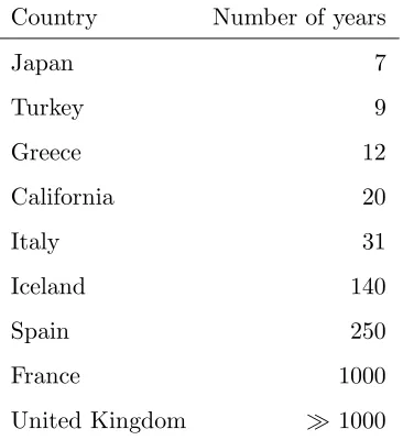
116
As demonstrated by the review of Douglas (2003a) many different choices,
117
in terms of dependent and independent variables, derivation technique and
118
functional form, were made by GMPE developers until the 1990s. In the
119
past couple of decades, however, there has been a general convergence to a
120
set ofde facto standards.
121
Most developers now present models for PGA, increasingly PGV, and
122
pseudo-SA for 5% of critical damping based on the geometric mean of the
123
values from two horizontal components, or the orientation-independent
hor-124
izontal component (Boore et al., 2006). They often use records from public
125
online databases (e.g. Akkar et al., 2014b; Chiou et al., 2008) that have
126
been low-cut filtered with record-specific cut-offs that are then respected
127
when considering the reliable frequency ranges of their models.
128
The size of an earthquake is invariably characterized in terms of
mo-129
ment magnitude (M), although this is sometimes estimated from other
mag-130
nitudes, commonly local magnitude (ML) (e.g. Bindi et al., 2005;
Goertz-131
Allmann et al., 2011), duration magnitude (Md) (e.g. Bakun, 1984; Edwards 132
and Douglas, 2014) or surface wave magnitude (Ms) (e.g. Ambraseys and
133
Free, 1997), through region-specific equations. Generally the earthquake is
134
characterized into three faulting mechanisms (styles of faulting): normal,
135
strike-slip and reverse. It is now common to consider nonlinear magnitude
scaling (see Section 4.2).
137
The length of the travel path from source to site is generally measured
138
either in terms of the distance to the surface projection of the rupture (the
so-139
called Joyner-Boore distance, rjb) (Joyner and Boore, 1981) or, accounting 140
for the depth, the distance to the causative fault (the so called rupture
dis-141
tance,rrup). For smaller earthquakes, where point sources can be assumed, 142
these distance metrics become equal to epicentral (repi) and hypocentral
143
(rhyp) distances, respectively. Some recent studies present models for both 144
finite-fault (rrup or rjb) and point-source (repi or rhyp) distance metrics so
145
that the correct GMPE is available when used within PSHA for point sources
146
(e.g. within area sources) (Bommer and Akkar, 2012) without having to
per-147
form conversions. It is also common to account for magnitude-dependent
148
decay of IMs with distance (see Section 4.2).
149
Because boreholes were typically drilled to 30 m and because of its
subse-150
quent use within many projects and design codes, e.g. Eurocode 8, the
time-151
average shear-wave velocity in the top 30 m (Vs,30) is the common way that
152
near-surface site conditions are characterized within recent GMPEs, either
153
directly or, when insufficient information is available, through site classes.
154
It is still relatively uncommon for GMPEs to account directly for potential
155
nonlinear site amplification because this behavior is rare within observed
156
strong ground motions. Within PSHA non-linear effects generally require
157
a simulation-based site term to be adopted, often from a stand-alone study
158
(Kamai et al., 2014; Seyhan and Stewart, 2014; Sandikkaya et al., 2013).
159
Finally it has become standard to use either random-effects
(Abraham-160
son and Youngs, 1992) or one- or two-stage maximum-likelihood regression
161
(Joyner and Boore, 1993) to estimate the free coefficients of the model.
162
These techniques, applied to the same data, would lead to very similar
results, although the latter may be more susceptible to trade-offs. Both
164
techniques provide estimates of the between- and within-event components
165
of ground-motion variability (see Section 5).
166
3. Additional independent variables
167
To obtain GMPEs that estimate more appropriate ground motions for a
168
given earthquake, path and site, independent variables in addition to
mag-169
nitude, faulting mechanism, source-to-site distance and a near-surface site
170
class (orVs,30) have been tested and/or included within some recent models.
171
These attempts are briefly discussed in this section.
172
3.1. Source parameters 173
All GMPEs include magnitude as the main source parameter. This is
174
now routinely moment magnitude due to its robustness, the fact that it
175
does not saturate, and because it is possible to estimate from historical and
176
palaeological information. The latter consideration is important in linking
177
GMPEs to earthquake catalogs, where the longer the available time-period
178
the more reliable are recurrence relations, particularly at higher magnitudes.
179
While magnitude is certainly an important factor for ground-motion
ampli-180
tudes, there are other source parameters that can control the amplitude and
181
frequency content of radiated seismic energy. The most influential of these
182
is the earthquake stress drop. While the stress drop has a physical
mean-183
ing, there are different definitions (e.g. static, dynamic or ‘Brune’). When
184
referred to in engineering seismology applications ‘stress drop’ or ‘stress
185
parameter’ is effectively used to refer to the proportion of high-frequency
186
energy (for a given magnitude) that is radiated from the source (Atkinson
187
and Beresnev, 1997).
Following on from observations of Somerville (2003), model developers of
189
the NGA West 1 and 2 projects (Power et al., 2008; Bozorgnia et al., 2014)
190
investigated the impact of depth to the top of the rupture plane (ZT OR) on
191
ground motions. Some of them (e.g. Campbell and Bozorgnia, 2014) find
192
that using ZT OR within the model leads to statistically better predictions
193
with deep earthquakes generating higher ground motions than shallow events
194
(all other things being equal), which could be explained by higher stress
195
drops. Possible lower stress drops for aftershocks is behind the decision of
196
some NGA West developers to exclude data from this type of event (e.g.
197
Boore and Atkinson, 2008) whereas others (e.g. Chiou and Youngs, 2008)
198
include terms to account for this difference. This effect appears to be small
199
and could be related to the way that earthquakes are classified (Douglas and
200
Halld´orsson, 2010). Radiguet et al. (2009) present evidence that SAs from
201
immature faults are statistically-significantly higher than those from mature
202
faults, which again could be related to higher stress drops for earthquakes
203
occurring on immature faults. The maturity of faults has yet to be included
204
in a GMPE because the age of faults is not a readily-available parameter.
205
The recent ground-motion model by Bora et al. (2015) includes an explicit
206
term for the stress (drop) parameter (∆σ) commonly used within stochastic
207
models (e.g. Atkinson and Silva, 2000; Rietbrock et al., 2013), while Douglas
208
et al. (2013) and Bommer et al. (2016) present unique GMPEs for a range of
209
∆σ. This allows models to be readily employed in areas where the average
210
stress drop is known but it puts the onus on the user to select an appropriate
211
median ∆σ (and uncertainty about this value).
212
Directivity of earthquake ground motion fields is an emerging topic that
213
has been addressed, for example, in the recent NGA West 2 project (Spudich
214
et al., 2014). While often clear in large-magnitude earthquake simulations,
this issue has seen relatively little focus in recent years. This is primarily due
216
to the nature of PSHA, which combines all possible earthquake scenarios:
217
rupture directivity effects, therefore, tend to be smoothed out. However, in
218
understanding deterministic hazard, or for future analyses, where rupture
219
directivity preference can be assigned, accounting for this effect may help to
220
reduce epistemic uncertainty.
221
3.2. Path parameters 222
Path terms within GMPEs have grown more complex in terms of their
223
functional form over the past decade with the realization that ground
mo-224
tions from small and large earthquakes do not decay at the same rate (see
225
Section 4.2). In addition, because of the availability of ground-motion data
226
(often from broadband instruments or high-sensitivity strong-motion
sen-227
sors) at distances greater than 100 km (roughly the limit of analogue
strong-228
motion recording) a number of GMPEs include terms to model anelastic
229
attenuation, the rate of which is sometimes considered regionally-dependent
230
(see Section 4). Cousins et al. (1999), for example, developed a GMPE
231
for New Zealand that accounts for additional attenuation for travel paths
232
through volcanic regions by including a term that is a function of the
hori-233
zontal distance through such zones.
234
Nevertheless, commonly travel path is simply parameterized using
source-235
to-site distance. This means that the decay rate is the same for all locations
236
irrespective of the crustal structure. Douglas et al. (2004, 2007) develop a
237
technique based on simulations to calculate an equivalent hypocentral
dis-238
tance that captures the impact of crustal structure on ground-motion decay
239
and, consequently, allows a ground-motion model to be branched into
region-240
specific models. This approach has yet to be applied for the derivation of a
GMPE for use in practice.
242
A handful of GMPEs (generally for use in California) include terms to
243
model the location of a site with respect to the hanging and foot walls of
244
the causative fault (e.g. Campbell and Bozorgnia, 2014; Abrahamson et al.,
245
2014), sometimes by usingRx (the horizontal, strike-normal distance to the
246
shallowest part of the surface projection of the fault). The terms to model
247
this effect are often complex and hence rely on simulations to constrain their
248
free parameters. For applications in areas without clearly-defined dipping
249
faults such terms are often turned off when the model is used within PSHA.
250
3.3. Site parameters 251
As discussed in Section 2.1, most current GMPEs useVs,30or site classes
252
based on Vs,30 to characterize the near-surface conditions at a site. In an
253
attempt to account for the effect of deeper structure on ground motions,
254
some recent GMPEs for California often use, in addition toVs,30, either the
255
depth to the 1 km/s velocity horizon (Z1.0) (e.g. Chiou and Youngs, 2014)
256
or the depth to the 2.5 km/s horizon (Z2.5) (e.g. Campbell and Bozorgnia,
257
2014). Z1.0 and Z2.5 are often strongly correlated but weakly correlated
258
withVs,30and hence their use alongsideVs,30adds discriminatory power to a
259
GMPE. For many parts of the world estimates ofZ1.0 and, particularly,Z2.5 260
are, however, difficult to obtain because they require knowing the shear-wave
261
velocity down to hundreds or thousands of meters. Consequently, empirical
262
relationships to estimate these parameters from Vs,30 have been proposed
263
(Boore et al., 2011) to center the predictions at an average Z1.0 or Z2.5.
264
PSHA is often conducted for a rock site with Vs,30 equal or larger than 265
760 m/s [the NEHRP B/C boundary (National Earthquake Hazard
Reduc-266
modeled in the GMPE will be low and any nonlinearity in modeled response
268
weak. One of the largest changes in PSHA for such sites in the past decade
269
has been the appreciation that site amplification related to shear-wave
ve-270
locity is not the whole story but that high-frequency attenuation, generally
271
modeled by κ (Anderson and Hough, 1984), also needs to be considered.
272
The effect of an average κ is implicitly captured within empirical GMPEs
273
through the data that are used. The averageκ implied by the shape of the
274
short-period spectra of GMPEs evaluated for high Vs,30 is, however, often
275
much higher than theκ measured at rock sites. Consequently, as discussed
276
in Section 4.5, a host-to-target adjustment for κ is required when these
277
GMPEs are used in a site-specific study. In an attempt to overcome this
278
requirement, Laurendeau et al. (2013) introduce a term for κ directly into
279
a GMPE developed from Japanese data. Use of such a model means that
280
κ needs to be known for a site of interest. This is the apparent drawback
281
of introducing new variables into GMPEs: the requirement for the user to
282
know their value and their uncertainty for their study. In the past, however,
283
the user generally assumed that the implicit average value within the data
284
used to derive the GMPE was appropriate for their site.
285
4. Regional models
286
With the rapidly-growing quantity of data from digital strong-motion
287
networks, which accurately record earthquakes down toM3 and below, there
288
has been a move towards the development of GMPEs for small geographical
289
regions (e.g. national or sub-national) and partially away from models
cov-290
ering large tectonic regimes, e.g. shallow crustal earthquakes globally. An
291
idea of the utility of this approach for the development of empirical GMPEs
Table 1: The number of years required to record fiftyMw ≥5 shallow earthquakes
as-suming dense strong-motion network covering whole territory (country or state) based on
the International Seismological Centre’s earthquake catalog from 1992 to 2012.
Country Number of years
Japan 7
Turkey 9
Greece 12
California 20
Italy 31
Iceland 140
Spain 250
France 1000
United Kingdom ≫ 1000
given only data from a country or state can be gained from Table 1. For
293
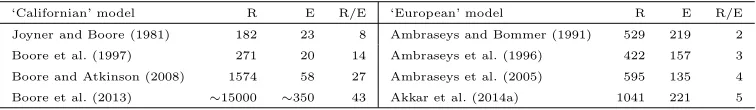
some highly seismically active areas this goal of purely-national GMPEs is
294
feasible but for less active (e.g. Spain) or smaller countries (e.g. Iceland)
lo-295
cal records would have to be used in conjunction with simulations or foreign
296
data to derive robust models.
297
As discussed in Section 4.2, there are difficulties in developing regional
298
models for use within standard seismic hazard assessments unless the models
299
are derived using data from large events. Therefore, to account for potential
300
regional dependency some GMPE developers derive a robust model using
301
data from a variety of regions within a single tectonic regime (e.g. shallow
302
crustal) and then add terms when required to account for observed regional
303
differences. For example, Boore et al. (2014) include terms to model
differ-304
ences in anelastic attenuation in China/Turkey and Japan/Italy to other
eas (predominantly California). In addition to regional variations in median
306
predictions, the variability of ground motion may be regionally-dependent.
307
For example, Abrahamson et al. (2014) differentiate between variability in
308
Japan and elsewhere.
309
Regional dependence of ground-motion models is, therefore, still a topic
310
of ongoing research. The issue is somewhat complicated by the sweeping
311
terms typically used to classify tectonic regions: stable continental, shallow
312
active crustal and so forth. Within each of these groups significant
variabil-313
ity in both structure and geology exists – meaning that systematic variability
314
in ground motion may be obscured if only looking at differences within or
315
between these classes. Nevertheless, it is generally acknowledged that at
dis-316
tances larger than around 50 km, regional variations in geology and tectonic
317
structure lead to significant differences in ground motion attenuation (e.g.
318
Boore et al., 2013; Kotha et al., 2016b,a). On the other hand, differences
319
at shorter distances are less well understood due to limited data and the
320
complexity of earthquake sources. Regional differences in stress fields due
321
to factors such as tectonic loading and structure (G¨olke and Coblentz, 1996),
322
or, at smaller scales, due to fault structure and maturity (Manighetti et al.,
323
2007) may lead to differences in earthquake stress drop that can be observed
324
at national (e.g. Goertz-Allmann and Edwards, 2014) or local scales (e.g.
325
Allmann and Shearer, 2007). The resolution of such analyses is, however,
326
debated due to the trade-off with attenuation, which is typically assumed to
327
be homogeneous. Addressing the issue of regionalization of ground-motion
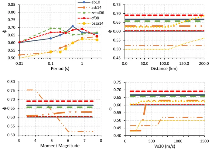
328
models requires more data, particularly at short distances. In the meantime,
329
hazard analysts can use hazard disaggregation to understand, to a first
or-330
der, the sensitivity of possible regional ground motions on seismic hazard.
331
For instance, hazard is often primarily driven by relatively close earthquakes
(<50 km) and, hence, regional differences in geology will be less important
333
to understand than differences in fault-rupture kinematics, for example.
334
4.1. Testing of GMPEs 335
When conducting a seismic hazard assessment for a region that is not
336
covered by a selected GMPE it has been increasing common to undertake
337
a quantitative comparison between predictions and the ground motions
ob-338
served in the region (Stewart et al., 2015). This has only become possible
339
for many parts of the world since the advent of digital ground-motion
net-340
works in the past couple of decades. Various methods have been developed
341
to undertake this testing but they are invariably based on ‘residuals’2, either 342
total or, more correctly, separated into between- and within-event
compo-343
nents (Stafford et al., 2008), between predictions and observations. The
344
most employed techniques are those by Scherbaum et al. (2004), Scherbaum
345
et al. (2009) and Kale and Akkar (2013). A more informative approach is to
346
consider plots of the residuals with respect to magnitude, distance and other
347
variables to understand what parts of the model are causing any misfits (e.g.
348
Scasserra et al., 2009).
349
A difficulty with such testing is that it is difficult to judge how much
350
weight should be given to a good or poor match as the available data are
351
often sparse and/or only available for magnitude and distance ranges of
352
limited engineering interest (Beauval et al., 2012). If a poor match is found
353
between observations and predictions and this is judged to be robust then
354
adjustment factors can potentially be derived to modify the GMPE so that
355
2They are not strictly residuals because generally the data compared were not used for
it provides better predictions (Bommer et al., 2006). This approach has
356
been formalized in the so called referenced-empirical technique by Atkinson
357
(2010) and variants of it have been applied in various projects, particularly
358
to adjust models for small and moderate events (e.g. Bourne et al., 2015).
359
4.2. Scaling of ground motions for small and large earthquakes 360
In the past decade there has been a push to derive GMPEs to predict
361
accurately ground motions from earthquakes with M<5. Until the
estab-362
lishment of digital strong-motion networks, which started in many regions
363
in the late 1990s, ground-motion databases generally became sparse below
364
aboutM5. In addition, for high seismicity areas, where most of the available
365
data are from, the dominant earthquake scenarios for engineering purposes
366
are generally at M > 5.5. Consequently there was little call for GMPEs
367
that could be used confidently for small earthquakes.
368
The development of such models in the past decade has been driven
369
by the availability of large sets of records from digital networks with good
370
coverage down to oftenM3 for many parts of Europe and elsewhere. Often
371
these data are used to derive regional GMPEs (see Section 4) generally
372
without the inclusion of data from larger earthquakes. When applying a
373
GMPE in a different geographical region than for which it was originally
374
derived it is important to check it against local data. As shown by, for
375
example, Douglas (2003b), unless the GMPE was derived using data from
376
small events and an appropriate functional form was used there will likely
377
be a large discrepancy between predictions and observations. This has been
378
used as an argument for a strong regional dependency in ground motions
379
but, as shown by Cotton et al. (2008) amongst others, it is likely due to the
380
differing magnitude ranges of the observations and model. Another recent
driver in the development of GMPEs that cover the range belowM5, even
382
for high seismicity zones, is the need for such models to estimate components
383
of the ground-motion variability that require many records from the same
384
site (see Section 5.3).
385
As shown by Douglas (2003b, Figure 4), Douglas and Jousset (2011)
386
and Baltay and Hanks (2014), empirical GMPEs derived from data from
387
small earthquakes generally show higher dependency on magnitude,
partic-388
ularly for short-period IMs, than those models derived for moderate and
389
large events. This means that extrapolation of these models beyond the
390
magnitude range for which they were derived often leads to over-prediction.
391
Fukushima (1996), Douglas and Jousset (2011) and Baltay and Hanks (2014)
392
demonstrate that a simple stochastic model (Boore, 2003) with a
single-393
corner source spectrum (Brune, 1970) and high-frequency attenuation
(An-394
derson and Hough, 1984) reproduces the observed magnitude-scaling of
em-395
pirical GMPEs and demonstrates why extrapolation of such models is so
396
problematic. Algorithmic differentiation (Molkenthin et al., 2014) can be
397
used to study the scaling of GMPEs with respect to its input parameters,
398
which aids understanding of how the models behave and extrapolate.
399
As well as magnitude-scaling being different for ground motions from
400
small and large earthquakes, the decay with distance also differs.
Earth-401
quake magnitude has two effects on the distance dependence of
ground-402
motion attenuation. The first is due to near-field saturation: as one
ap-403
proaches a finite source, the contribution from the far ends of the source
404
become increasingly small due to the distance that the energy must
propa-405
gate to reach you (attenuation effects) and the time which this takes
(scat-406
tering and dispersion effects). At short and moderate structural periods,
407
therefore, the peak amplitudes of a M7 event are similar to an M8. The
primary difference is the duration and spatial extent over which the
mo-409
tions occur, being significantly longer and more widespread in the latter
410
case. The second effect is the distance dependence of the ground motion
411
decay. For increasingly large events the finite nature of the source means
412
that ground motion does not decay as quickly as for small (roughly point)
413
sources, since the motion at distance is increased by constructive
interfer-414
ence from later arrivals along the finite fault (e.g. Boore, 2009). In fact,
415
even for point-source models, Cotton et al. (2008) showed that the decay
416
of response spectral ordinates is magnitude-dependent due to the influence
417
of spectral shape. To capture this, functional forms of GMPEs in the past
418
decade have often used magnitude-dependent decay terms.
419
4.3. Non-tectonic earthquakes 420
Although the vast majority of GMPEs are still derived for tectonic
earth-421
quakes, a growing number of models are available for earthquakes of other
422
types, e.g. those induced by mining (e.g. McGarr and Fletcher, 2005) or
423
fluid injection (e.g. Douglas et al., 2013). Seismic hazard assessments for
424
human-activity-related, induced or triggered earthquakes require
ground-425
motion models that are adapted to this type of event and it is not a priori 426
clear that shaking from such shocks is similar to that from natural
earth-427
quakes. In addition, the magnitude, source-to-site distance and focal depth
428
range of importance for induced seismicity is generally smaller than the
fo-429
cus of hazard assessments for natural earthquakes. Hence, as discussed in
430
Section 4.2, this leads to the need to develop models to account for this
dif-431
ference. The finding of Douglas et al. (2013) that motions from induced and
432
natural shallow seismicity are statistically similar means that the more
abun-433
dant data banks of records from small natural shallow earthquakes could be
used to derive GMPEs for use within hazard assessments for induced
seismic-435
ity (e.g. Atkinson, 2015). It could also be argued that with an appropriate
436
correction for depth [i.e. for distance and stress-drop (Hough, 2014)], data
437
from deeper natural seismicity could be used to determine ground-motion
438
fields of larger induced events.
439
4.4. Prediction for a reference velocity horizon 440
Ground motion within PSHA is typically estimated for a reference site,
441
circumventing the geological heterogeneity of the uppermost layers. This
442
is often at or around the NEHRP class B/C boundary of 760 m/s or the
443
Eurocode 8 class A/B boundary of 800 m/s (e.g. Delavaud et al., 2012).
444
Subsequently, the results of microzonation or site-specific response analyses
445
can be applied in conjunction with these estimates. The reason for this is the
446
significant variability of resolution, reliability and availability of site-specific
447
data. Practitioners are, in this way, free to apply their own site specific
448
corrections to a regionally-consistent hazard map for reference rock.
449
Site response terms within GMPEs are included for two reasons. Firstly,
450
to enable ground-motion records from all site conditions (including
non-451
rock stations, which comprise the majority of most strong-motion networks)
452
to be used to derive GMPE that would be statistically more robust than
453
using only rock records. A few developers (e.g. Idriss, 2014) exclude records
454
from sites with low Vs,30 because they believe that it is not possible to
455
capture site response by means of a simple site term. Consequently such
456
models are generally based on far fewer records but the risk of bias from
457
site amplification is reduced. The second reason for including site terms in
458
GMPEs is that such models allow seismic hazard assessments for a variety
459
of sites (including non-rock sites) to be easily conducted, which could be
useful when high accuracy is not a requirement.
461
In a similar way, recent PSHAs (e.g Bommer et al., 2015) predict the
462
ground motion initially at a subsurface reference rock horizon, choosing a
463
depth below which lateral variability is considered insignificant (usually at a
464
wave velocity consistent with ‘engineering’ or hard rock). Site-specific
non-465
linear amplification is then applied during the hazard calculation based on
466
site-response analyses. This approach has the benefit of potentially reducing
467
the site-to-site variability in predicted ground motion. If one assumes the
468
full range of site variability is captured through this process then the GMPE
469
component of site-to-site variabilityφS2S (see Section 5.3) can be set to zero, 470
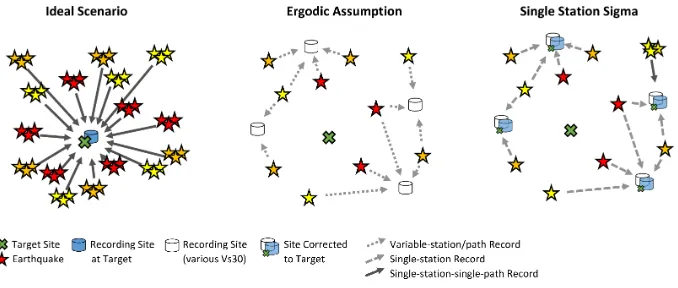
leading to non-ergodic single-station sigma (Atkinson, 2006). Practitioners
471
must be careful in this case that the modeled variability of the site response
472
is sufficient, but at the same time not so high that ergodicσs are exceeded
473
due to uncertainty in site response analyses.
474
The move towards reference-site hazard and reference horizons to make
475
best use of site-response analyses means that GMPEs are being increasingly
476
evaluated for relatively highVs,30(e.g. ≥760 m/s). This is one of the factors
477
driving the derivation of new GMPEs. Sites with high Vs,30, however, are
478
poorly represented in strong-motion databases because many stations are
479
installed in urban environments on soft and stiff soils (e.g. Akkar et al.,
480
2010).
481
4.5. Host-to-target adjustments 482
Ground motion is dependent on the shear-wave velocity and attenuation
483
characteristics of the upper layers of soil and rock. When modifying site
484
conditions, e.g. changing predictions relevant for California to a site-specific
485
target in the United Kingdom, hazard analysts must consider the effect of
this change on the predicted ground motion. This is done through
host-to-487
target adjustments.
488
As stated above, GMPEs are typically developed using site descriptors
489
such as class (e.g. rock, stiff soil and soft soil) or Vs,30. It is important 490
to note, however, that when using a GMPE estimates are implicitly tied
491
to a range of possible site types that fall within the site descriptor and
492
this may be biased by a particular geology. Even GMPEs usingVs,30 will
493
cover a range of site types because many velocity profiles are possible for a
494
givenVs,30. While different velocity profiles can lead to the sameVs,30, they
495
may lead to significantly different amplifications (e.g. Castellaro et al., 2008;
496
Papaspiliou et al., 2012). If a particular velocity structure (e.g. low velocity
497
soils over a high velocity basement) is characteristic of a region, then ground
498
motion at a Vs,30 in one region may be systematically different to that in
499
another with a different average structure. As discussed previously, some of
500
this site variability can be captured by using additional site parameters, such
501
as Z1.0 or Z2.5. Recent PSHA studies have, however, moved towards fully
502
accounting for the effect of site-specific characteristics, by taking advantage
503
of the wealth of information often available for site-specific hazard analyses.
504
Such differences are accounted for by using host-to-target adjustments. The
505
same approach can be used to modify ground-motion predictions made at a
506
particularVs,30 and provide them at another. This approach is particularly
507
useful in the case that GMPE predictions are considered unreliable at the
508
targetVs,30.
509
Since earthquake engineering generally uses SA, direct adjustments of the
510
Fourier amplitude spectra (FAS) cannot be used to perform host-to-target
511
adjustments. This is because ground motion at a given oscillator period is
512
dependent not only on the FAS at that period but also other values around
it (e.g. Bora et al., 2015). The host-to-target ratio is, therefore, dependent
514
on the input ground motion in addition to the different site properties. The
515
hybrid-empirical method (HEM) based on Campbell (2003) is commonly
516
used to make host-to-target adjustments. HEM uses stochastic simulations
517
[typically using random-vibration theory (RVT) (Cartwright and
Longuet-518
Higgins, 1956)] to generate FAS-compatible response spectra for the host
519
and target sites, which can then be used to calculate the ratio in terms of
520
SA.
521
Using RVT through the HEM allows transformations from the Fourier
522
domain into the response spectral domain. HEM, however, requires a full
523
seismological model (for source, path and site) of the host and target
re-524
gions. Because of this Al Atik et al. (2013) developed a method based on
525
inverse RVT (IRVT) (Vanmarcke and Gasparini, 1976) that can be used to
526
modify response spectra for host-to-target adjustments in the Fourier
do-527
main. The method has the advantage that no assumptions on the form
528
of the host model (GMPE) are required. Working in the Fourier domain
529
has the advantage that adjustments are independent of the input motion
530
unlike when working in the response spectral domain. For a given signal
531
duration (often defined based on simple regional models), IRVT transforms
532
the response spectrum into a compatible FAS. FAS based host-to-target
533
conversion can then be applied to the response-spectrum-compatible FAS
534
before being returned to the response domain through the standard RVT
535
approach. A limitation of the IRVT approach is that the response spectrum
536
becomes less sensitive to the FAS as oscillator period decreases. This results
537
in significant non-uniqueness of the response-spectrum-compatible FAS at
538
short periods (roughly T < 0.05 s). Nevertheless, an advantage of this
ap-539
proach is that one can directly estimate seismological parameters from the
GMPE-compatible FAS, such asκ.
541
Figure 2 shows an application of the Vs-κ0 corrections to GMPEs used 542
in the Swiss National Seismic Hazard Maps (Edwards et al., 2016). The
543
selected targetVsprofile (Poggi et al., 2011, Vs,30= 1105 m/s) andκ0 value 544
(Edwards et al., 2011,κ0 = 0.016 s) define the reference rock for the seismic
545
hazard map. For each GMPE two possible host Vs profiles were selected
546
(with definedVs,30 where the GMPE’s developers considered the best data
547
coverage for rock). Fourκ0 values were also selected for each GMPE using
548
eitherVs,30-κ0correlations or direct measurement using IRVT. The resulting
549
eight Vs-κ0 corrections for each GMPE were considered to represent the
550
epistemic uncertainty involved in adjusting GMPEs to the regional reference.
551
Small but significant differences arise at long periods due to differences in
552
amplification of the host-Vs profiles. Far more significant, however, is the
553
epistemic uncertainty evident in the correction at short periods (T <0.1 s),
554
which is due to the uncertainty in definingκ0 (e.g. Edwards et al., 2015).
555
Similar observations are made by Rodriguez-Marek et al. (2014) for a
site-556
specific hazard assessment.
557
5. Aleatory variability
558
Over the past decades there has been a growing realization that
predict-559
ing shaking in future earthquakes is associated with large uncertainties and
560
that this uncertainty must be captured within seismic hazard assessments.
561
It has become standard to split these uncertainties into two components:
562
those of inherent randomness, referred to as aleatory variability (this
sec-563
tion) and those relating to a lack of knowledge or understanding, referred
564
to as epistemic uncertainty (Section 6).
Figure 2: Vs-κ0 corrections proposed for the Swiss National Seismic Hazard Maps by
Edwards et al. (2016). Blue/Red indicate different hostVsprofiles (two for each GMPE),
line types indicate differentκ0(four for each GMPE) resulting in eight possible corrections
per GMPE. AB10: Akkar and Bommer (2010); CF08: Cauzzi and Faccioli (2008); CY08:
Chiou and Youngs (2008); and Zetal06: Zhao et al. (2006). The target properties are
The definition of aleatory (and consequently epistemic) variability
in-566
evitably leads to disagreement and confusion. It could be argued, for
in-567
stance, that given a perfect model, aleatory variability is, by definition,
568
zero. However, in current understanding we can at least separate the
vari-569
ability into parts that can be quantified in terms of scientific uncertainty (e.g.
570
using different models to predict the same phenomena, such as site
ampli-571
fication), and those for which there is (at least currently) no
scientifically-572
based predictive capability (e.g. the stress-drop of the next earthquake). A
573
more appropriate terminology may therefore beapparent aleatory
variabil-574
ity with respect to a chosen model (written communication, J. J. Bommer,
575
2016). The advantage of splitting uncertainty into constituent components
576
is that the logic-tree approach (Kulkarni et al., 1984) can then be used
577
to branch through the epistemic uncertainty space (e.g. by selecting and
578
weighting different models) and allowing site or region-specific selections to
579
be made along with sensitivity studies and analyses (e.g. disaggregation) at
580
a branch-by-branch level. The distinction between aleatory and epistemic
581
is particularly important, for example, in the case of a fully probabilistic
582
seismic risk (or safety) assessment for a safety critical structure such as a
583
nuclear power plant. Such assessment requires the fractiles of the hazard
584
to be defined, which can only be correctly calculated with an appropriate
585
separation of aleatory and epistemic uncertainty.
586
Following Douglas (2003a), Strasser et al. (2009) observe that σ
associ-587
ated with GMPEs has shown little or no decrease since the 1970s despite
588
the increasing complexity of models. This fact and the importance of σ on
589
the results of PSHAs at long return periods, has encouraged attempts to
590
increase the complexity of models to account for other effects than simply
591
magnitude, distance and site class (see Section 3). To date these attempts
have not led to significant reductions in σ because GMPEs remain simple
593
representations of complex physical phenomena. Improvements to metadata
594
do, however, lead to slight reductions in assessedσ. For example, the model
595
of Chiou and Youngs (2014) is associated with a smallerσ when measured
596
Vs,30 is used for a site than when an estimate of this site parameter is
em-597
ployed.
598
One of the major areas of engineering seismology research in the past
599
decade has been in separatingσinto its different components (Al Atik et al.,
600
2010; Lin et al., 2011; Rodriguez-Marek et al., 2013) and using the
appro-601
priate components when conducting a hazard assessment (e.g. Walling and
602
Abrahamson, 2012). There has also been a move from using whatever data
603
were available towards selecting to: limit bias, exclude unreliable data, make
604
analysis easier, and obtain more reliableσestimates. As noted above, it has
605
become standard to use random-effects/maximum-likelihood methods to
es-606
timate between-event (τ) and within-event (φ) components.
607
Records from nearby sites are correlated, which has been recognized by
608
Jayaram and Baker (2010) when developing a regression technique to
ac-609
count for spatial correlations and by Boore et al. (1993), who choose only
610
a single record per site class within a radius of 1 km. These spatial
corre-611
lations are also important when conducting PSHA for infrastructure with
612
considerable spatial extent or when computing group earthquake risk over
613
an extended area.
614
5.1. Between-event variability 615
Aleatory variability within a given GMPE is usually separated into
616
between- and within-event components (τ and φ, respectively).
Between-617
event terms (random-effects in the context of random-effects regressions),
which are source-specific, are thought to be mainly related to stress drop
619
(Cotton et al., 2013). Using stochastic simulations, Drouet and Cotton
620
(2015) showed that the between-event variability was strongly controlled
621
by the stress parameter (as noted previously, ‘stress parameter’ is used to
622
avoid physical interpretation in terms of pure ‘stress drop’ and rather
in-623
dicate the proportion of high-frequency energy radiated by an earthquake).
624
The between-event term can, therefore, be thought of as describing how
625
energetic the rupture was compared to the average for a given magnitude
626
(all other things being equal). Such features are not possible (currently)
627
to predict and, therefore, fall into the category of aleatory variability. The
628
standard deviation of these event terms is described byτ.
629
One of the main ways GMPEs are improving is related to the
record-630
ing of each earthquake by an increasing number of stations (in particular,
631
fewer singly-recorded events) so that the source terms (and τ) are better
632
constrained. This is particularly true for models based on predominantly
633
Californian or Japanese data but much less so for models derived from data
634
from Europe and the Middle East (Table 2 and Figure 3). This shows
635
that despite recent improvements in strong-motion networks in Europe and
636
Middle East, strong motion databases there remain dominated by
poorly-637
recorded events. For models based on data with low record-to-event ratios
638
the source terms (e.g. style-of-faulting factors) andτ are poorly constrained.
639
Additionally, the small number of well-recorded events have a strong
influ-640
ence on the model.
641
τ is often found to be heteroscedastic, with decreasing variability as
mag-642
nitude increases (e.g. Youngs et al., 1995) (Figure 4). Estimated
ground-643
motion variability from small events (M < 5) is often significantly larger
644
than at moderate and large magnitudes, with many GMPE developers
Chuetsu-oki, Japan Niigata, Japan Tottori, Japan Chi-Chi, Taiwan Iwate, Japan El Mayor-Cucapah 10370141 10275733 14312160 Anza-02 14383980 Wenchuan, China 10410337 40199209 40204628 Northridge-01 71336726 14138080 Parkfield-02 14151344 21522424 14186612
Percentage of complete dataset
0 1 2 3 4
Campbell & Bozorgnia (2014)
15521 records, 321 earthquakes
Top third: 5264 records, 22 earthquakes
0 100 200 300 400 500 600
2008 June 13 23:43
1999 September 20 17:47
2007 September 30 17:21
1997 May 13 05:38
2005 April 19 21:11
1997 March 26 08:31
2000 October 08 04:17
2004 October 27 01:40
2007 March 25 00:42
2003 July 25 22:13
2003 July 26 07:56
Cauzzi et al. (2015)
Total: 1878 records, 98 earthquakes
Top third: 669 records, 11 earthquakes
0 25 50 75
20110519201523 19990913115530 19991112165721 19990817000139 19991111144123 20061024140022 19790415061941 19801123183453 19990831081049 19971014152309 19991112171650 20071109014305 20000823134128 20090407174737 20090409005259 19801123193500 19970926094025 19991107165441 19760915092118 19971006232453 19971118130741 19990907115651 19991111145526 19991119102801 19991220032720 20061025115605 20090409193816 19900620210008 19990819151745 19991112220112 19991113083343 20000120103559
Bindi et al. (2014)
1291 records, 273 earthquakes
Top third: 435 records, 32 earthquakes
Number of records
[image:30.595.130.417.130.586.2]0 10 20 30 40 50
Figure 3: Number of records (bottom axes, different scales for all three subplots) and
percentage of total (top axes, same scales for all three subplots) from earthquakes
con-tributing to the top third of total number of records to three recent GMPEs: Campbell and
Bozorgnia (2014) (predominantly Californian data), Cauzzi et al. (2015) (predominantly
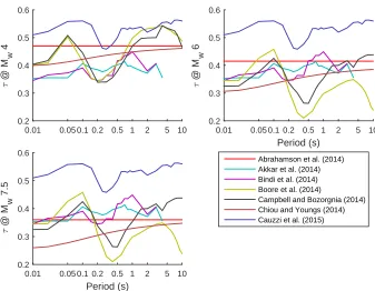
Table 2: Ratio (R/E) of number of records (R) per event (E) for four generations of
‘Californian’ and ‘European’ models.
‘Californian’ model R E R/E ‘European’ model R E R/E Joyner and Boore (1981) 182 23 8 Ambraseys and Bommer (1991) 529 219 2 Boore et al. (1997) 271 20 14 Ambraseys et al. (1996) 422 157 3 Boore and Atkinson (2008) 1574 58 27 Ambraseys et al. (2005) 595 135 4 Boore et al. (2013) ∼15000 ∼350 43 Akkar et al. (2014a) 1041 221 5
ing using data from small earthquakes. This is despite the need for models
646
at lower magnitudes, e.g. for seismic hazard assessment from induced
seis-647
micity, to examine the applicability of a GMPE in a new region and to
648
study the various components of ground-motion variability. While models
649
of ground-motion variability have improved significantly in recent years, we
650
must be careful not to over-interpret features of these models due to the
651
limitations of separating the different contributions. In Figure 4 there is
652
a peak at 0.1 s for several models which is difficult to understand in terms
653
of source variability. During the Hanford PSHA (Hanford.gov, 2014) this
654
was demonstrated to be an effect of sampling different ranges of site
re-655
sponse from event to event. The site variability is, therefore, mapped into
656
between-event terms leading to the peak at 0.1 s.
657
Arguments for observing lower variability at large magnitudes include
658
the fact that meta-data for large events (e.g. magnitude, depth and
mech-659
anism) are more reliable. While this is, in general, true, there has been
660
significant work in recent years to develop reliable earthquake catalogs for
661
smaller events. Another argument is that, due to large earthquakes having
662
large rupture sizes, the sensitivity of ground motion to, for example depth or
663
magnitude, is less. For example,M<5 events can generally be assumed to
664
be point sources, with amplitudes decaying in proportion to the reciprocal of
665
hypocentral distance. On the other hand,M>6 events emit waves from a
range of sources along several kilometers of rupture. Increasing the depth or
667
size of this fault, whilst changing the distance over which some of the seismic
668
energy must propagate, will, therefore, have a reduced effect. This is evident
669
in the saturation of ground-motion amplitudes for increasing magnitude in
670
GMPEs. Having reliable meta-data for larger events is, therefore, arguably
671
less important than for small earthquakes for sites not close to major active
672
faults. For other locations, reliable information on fault geometry and other
673
properties (e.g. rupture mode) is vital when estimating near-source ground
674
motions.
675
The limited number of events at large magnitudes leavesτ open to
under-676
sampling (with each event only contributing a single data-point to the
esti-677
mate ofτ). Given that strong-motion databases often include only a handful
678
of well-recorded events with M>7, the reliability of heteroscedasticτ can
679
be called into question. Comparing values from different GMPEs we can see
680
that the variability inτ estimates is rather high (Figure 4). In reality, τ is
681
likely to be heteroscedastic, but caution should clearly be applied in using
682
low values at M > 7.5 coming from extrapolation of trends from smaller
683
magnitudes (Musson, 2009). Models developed with constant τ estimates
684
forM<5 and M>7 connected by a linear trend (e.g. Abrahamson et al.,
685
2014) are an appropriate compromise in this sense.
686
5.2. Within-event variability 687
Ground-motion variability with respect to a given GMPE for single event
688
is described by within-event variability (φ). It can be interpreted as
describ-689
ing the standard deviation of the misfit between GMPE and data after
ac-690
counting for the between-event terms. In terms of the random-effects
frame-691
work, φ describes the standard deviation of within-event random-effects.
0.01 0.05 0.1 0.2 0.5 1 2 5 10
τ
@ M
w
4
0.2 0.3 0.4 0.5 0.6
Period (s)
0.01 0.05 0.1 0.2 0.5 1 2 5 10
τ
@ M
w
6
0.2 0.3 0.4 0.5 0.6
Period (s)
0.01 0.05 0.1 0.2 0.5 1 2 5 10
τ
@ M
w
7.5
0.2 0.3 0.4 0.5 0.6
Abrahamson et al. (2014) Akkar et al. (2014) Bindi et al. (2014) Boore et al. (2014)
[image:33.595.127.464.219.481.2]Campbell and Bozorgnia (2014) Chiou and Youngs (2014) Cauzzi et al. (2015)
Figure 4: Comparison of theτ models of six recent GMPEs: Abrahamson et al. (2014),
Boore et al. (2014), Campbell and Bozorgnia (2014) and Chiou and Youngs (2014)
(pre-dominantly Californian data); Bindi et al. (2014) and Akkar et al. (2014a) (European and
the Middle Eastern data); and Cauzzi et al. (2015) (Japanese data), for M4, 6 and 7.5
The logarithm of ground-motion variability is assumed to be normally
dis-693
tributed. The total variability of a dataset with respect to a GMPE is then
694
given by (assuming independence between the two components): pτ2+φ2.
695
Within-event variability is related to path and site phenomena in addition to
696
any spatially-dependent source characteristics, such as radiation pattern or
697
directivity effects. Because of the dominant effect of site amplification and
698
the significant variability of site effects these are considered to be a
signif-699
icant source of within-event variability (e.g. Rodriguez-Marek et al., 2011).
700
In the most recent studies, φ is therefore split into components describing
701
site-to-site variability (φS2S) and within-site variability (φ0). Drouet and 702
Cotton (2015) showed that the within-event variability is controlled by a
703
number of factors: the most significant being site amplification/attenuation
704
effects (includingκ) followed by path effects, such as geometrical and
anelas-705
tic attenuation. Bindi et al. (2014) observe that certain stations contribute
706
a large proportion of the soft soil (Eurocode 8 class D) sites for European
707
GMPEs. Some often-triggered stations, therefore, have strong influence on
708
the model and may reduce the apparent within-event variability.
709
While φ is often considered a ‘site term’ it is also observed to be
mag-710
nitude, distance and Vs,30 dependent (Figure 5). For instance, Boore et al.
711
(2014) and Campbell and Bozorgnia (2014) show thatφdecreases with
mag-712
nitude at short periods and increases with magnitude at long periods. Due
713
to the interaction of ergodic and non-ergodic components of variability it is
714
difficult to know if this is truly a site-specific effect or due to site-to-site
vari-715
ability (different sites having recorded different ranges of earthquake
magni-716
tudes and distances). An effective magnitude-distance dependence ofφdue
717
to nonlinearity of soil response has been incorporated into GMPE
develop-718
ment. For example, Abrahamson et al. (2014) account for soil non-linearity
Figure 5: Comparison of estimates of the within-event variability φ from some recent
GMPEs, where ab10 corresponds to Akkar and Bommer (2010), ask14 corresponds to
Abrahamson et al. (2014), zetal06 corresponds to Zhao et al. (2006), cf08 corresponds to
Cauzzi and Faccioli (2008) and bssa14 corresponds to Boore et al. (2014).
reducing the variability of short-period motions. Focusing on non-ergodic
720
sigma, Rodriguez-Marek et al. (2013) present models for single-station φ
721
using data from various tectonic regions. They show a decrease of
single-722
stationφover all periods, which differs from the observations of ergodic
vari-723
ability, where long-period motions show increasedφfor large earthquakes.
724
An explanation for the different observations of φ’s dependency on
dis-725
tance and magnitude may be found in the dependence of response spectral
726
amplification on the input motion (e.g. Bora et al., 2016). Given that
res-727
onance effects in site response depend greatly on the site type (e.g.
long-728
period resonance for deep sedimentary basins and high-frequency resonance