Contents lists available atScienceDirect
Automatica
journal homepage:www.elsevier.com/locate/automatica
Brief paper
A model predictive control approach to the periodic implementation of the
solutions of the optimal dynamic resource allocation problem
✩Jiangfeng Zhang
,
Xiaohua Xia
∗Centre of New Energy Systems, Department of Electrical, Electronic and Computer Engineering, University of Pretoria, Pretoria 0002, South Africa
a r t i c l e i n f o
Article history:
Received 21 November 2009 Received in revised form 5 May 2010
Accepted 21 September 2010 Available online 27 November 2010
Keywords:
Model predictive control Perfect optimal dynamic resource
allocation problem Energy optimization
a b s t r a c t
This paper proposes a model predictive control (MPC) approach to the periodic implementation of the optimal solutions of a class of resource allocation problems in which the allocation requirements and conditions repeat periodically over time. This special class of resource allocation problems includes many practical energy optimization problems such as load scheduling and generation dispatch. The convergence and robustness of the MPC algorithm is proved by invoking results from convex optimization. To illustrate the practical applications of the MPC algorithm, the energy optimization of a water pumping system is studied.
©2010 Elsevier Ltd. All rights reserved.
1. Introduction
There is a particular class of problems in resource allocation and energy appliance scheduling pertaining to special periodic constraints in minimizing objective functions. This class of prob-lems includes the scheduling of appliances (pumps, conveyor belts, generators, etc.) on a daily or weekly basis. The demand, opera-tion condiopera-tions, and constraints change only periodically during this time. For the purpose of this paper, this class of problems are calledOptimal Dynamic Resource Allocation Problems(ODRAP). Such problems will usually be solved over one period, e.g. 24 h, and the optimal solution will be repeatedly implemented for other periods without considering interactions between periods ( Mid-delberg,Zhang, & Xia, 2009). The interaction between periods of implementation is what makes the ODRAP different from those re-source allocation and scheduling problems generally studied (see Aissi, Bazgan, and Vanderpooten(2009),Belfares, Klibi, Lo, and Gui-touni (2007),Biegler and Zavala(2009),Ibaraki and Katoh(1988), Lee, Kumara, and Gautam(2007), Lee and Lee(2006),Munawar and Gudi(2005),Pasadyn, Lee, and Edgar(2008),Patriksson(2008) andZafra-Cabeza, Ridao, and Camacho(2008) and the references therein). In these papers, the research is focused on developing various algorithmic approaches to resource allocation problems
✩ The material in this paper was not presented at any conference. This paper was
recommended for publication in revised form by Associate Editor Lalo Magni under the direction of Editor Frank Allgöwer.
∗Corresponding author. Tel.: +27 12 4202165; fax: +27 12 3625000.
E-mail addresses:[email protected](J. Zhang),[email protected](X. Xia).
in which periodic constraints may not exist. Even though periodic constraints are included in the problem, the corresponding back-grounds are either not applicable to ODRAP or not explicitly dis-cussed. A lack of discussion particularly pertaining to the periodic implementations of optimal solutions for periodic resource alloca-tion problems exists. There may, in fact, be unintended interacalloca-tions between two periods when an optimal solution of an ODRAP for one period is implemented over consequent periods. A ramp rate violation, for example, may occur when the optimal solution of the dynamic economic dispatch (DED) problem over the first day (Xia, Zhang, & Elaiw, 2009) is simply implemented in the second day. This ramp rate violation actually implies that the constraints in an ODRAP formulation for DED are inadequate for periodic implemen-tation. This problem is solved by introducing more constraints and thus formulating a new ODRAP, or aPerfect Optimal Dynamic Re-source Allocation Problem(PODRAP). Furthermore,Xia et al.(2009) also proposes an algorithm to solve this revised dynamic economic dispatch problem by the model predictive control (MPC) approach. The same approach will be extended to the general PODRAP in this paper.
The ability of the MPC to handle constraints, being able to use simple models, and its closed-loop stability and inherent robustness makes it very practical for use in industrial problems (seeAllgöwer and Zheng(2000),Garcia, Prett, and Morari(1989), andQin and Badgwell(2003)). This MPC approach is also applied in general resource allocation or scheduling problems as done in Ferrari-Trecate et al.(2004),Lee et al.(2007),Lee and Lee(2006), Munawar and Gudi(2005), van Staden, Zhang, and Xia(2009), andZafra-Cabeza et al.(2008). It is interesting to note that MPC algorithms have a close relationship with optimization since an
MPC algorithm needs to solve an optimization problem in each iteration. Studies on the connections of MPC with optimization were conducted since the 1960’s (seeChang and Seborg(1983) and Zadeh and Whalen (1962)). Modern MPC approaches for resource allocation problems do not take the relationship of the MPC solutions and the global optimal resource allocation solutions into consideration.
The aim of this paper is to develop an MPC algorithm for the periodic implementation of the optimal solutions of the PODRAP. Further it will prove the algorithm’s convergence and the corresponding robustness against disturbances in controller implementation or state measurement. The convergence result reveals that the optimal solutions in the MPC algorithm converge to the optimal solution of the PODRAP. The formulation of PODRAP and the perfection of ODRAP can be found in Section2, while the convergence and robust results are in Section3. An example on the voluntary load shedding problem for a water pumping system is also studied in Section4to illustrate the formulation of a PODRAP and the convergence and robustness of the MPC approach. Some concluding remarks are drawn in the last section.
The following nomenclatures are fixed.
∑
ki=jaiequals 0 forj
>
kandaj+ · · · +
akifj≤
k;col
(α
1, α
2, . . . , α
s)
equals(α
T1, α
T2, . . . , α
sT)
T for any columnvectors
α
1, α
2, . . . , α
s;s.t.: subject to;
m
,
p,
n: fixed positive integersk
,
j: thek-th orj-th sampling time interval;(
k,
k+
p]
: the time interval fromktok+
pexcludingk;Xij: a 1-dimensional real variable for alli
,
j;X
[
j]
: them-dimensional real vector variable for allj;X
[
k|
j]
: the prediction ofX[
k]
at timejfor anyk≥
j;Z
[
k]
: equals col(
X[
k]
,
X[
k+
1]
, . . . ,
X[
k+
p−
1]
)
;Z
[
k|
j]
: the prediction ofZ[
k]
at timejfor anyk≥
j;ujk: equalsX
[
k+
1|
j] −
X[
k|
j]
;u
[
k|
j] :=
col(
ukj,
ujk+1, . . . ,
ujk+p−1)
=
z[
k+
1|
j] −
z[
k|
j]
;i1
,
i2, . . . ,
is: integers with 1≤
i1<
i2<
· · ·
<
is=
n;x
:=
(
x1,
x2, . . . ,
xn)
∈
Rn;yℓ
:=
(
xiℓ−1+1,
xiℓ−1, . . . ,
xiℓ), ℓ
=
1,
2, . . . ,
s, are calledpartitionsofxsuch thatx
=
col(
y1,
y2, . . . ,
ys)
.2. Problem formulation
PODRAP
(
k,
k+
p]
For any give system dynamicsX[
k+
1] =
G
(
X[
k]
)
, a PODRAP over the time interval(
k,
k+
p]
is defined as the minimization problem:min Jk+1
(
z[
k+
1|
k+
1]
)
s.t. Hk+1
(
z[
k+
1|
k+
1]
)
≥
0,
(1)where the optimization variable isz
[
k+
1|
k+
1] =
col(
X[
k+
1
|
k+
1]
,
X[
k+
2|
k+
1]
, . . . ,
X[
k+
p|
k+
1]
)
, and Jk+1 and Hk+1are smooth, convex functions satisfying the followingperiodic invariantproperties for allk≥
0:•
Periodic invariant objective:Jk+1
(
X[
k+
1]
,
X[
k+
2]
, . . . ,
X[
k+
p]
)
=
Jk+2(
X[
k+
2]
, . . . ,
X[
k+
p]
,
X[
k+
1]
),
(2)•
Periodic invariant constraints:{
(
X[
k+
1]
,
X[
k+
2]
, . . . ,
X[
k+
p]
)
:
Hk+1
(
X[
k+
1]
,
X[
k+
2]
, . . . ,
X[
k+
p]
)
≥
0}
= {
(
X[
k+
1]
,
X[
k+
2]
, . . . ,
X[
k+
p]
)
:
Hk+2
(
X[
k+
2]
,
X[
k+
3]
, . . . ,
X[
k+
p]
,
X[
k+
1]
)
≥
0}
.
(3)
Definition 1. Fix the notations in PODRAP
(
k,
k+
p]
, then the minimization problem (1)is called an optimal dynamic resource allocation problem(ODRAP) if the functionsJℓandHℓare smooth, convex, andJℓsatisfies the periodic invariant property(2)for allℓ
≥
1.Note that the only way in which the ODRAP and PODRAP differ is that an ODRAP may not satisfy the constraints in(3). A practical resource allocation problem may be an ODRAP but not a PODRAP, and the constraints can often be reasonably extended so that the periodic invariant property is satisfied (Xia et al., 2009).
The following two propositions are easy to verify and the proofs are omitted.
Proposition 1. Assume that there exists smooth and convex func-tions
α
i, β
i,
i≥
1, such thatα
i+p≡
α
i, β
i+p≡
β
i, and Jk+1and Hk+1have the following special form:Jk+1
(
X[
k+
1|
k+
1]
, . . . ,
X[
k+
p|
k+
1]
)
=
k+p−
i=k+1
α
i(
X[
i|
k+
1]
),
Hk+1
(
X[
k+
1|
k+
1]
, . . . ,
X[
k+
p|
k+
1]
)
=
k+p−
i=k+1
β
i(
X[
i|
k+
1]
).
Then the following optimization problem is a PODRAP over the time period
(
k,
k+
p]
min Jk+1
(
z[
k+
1|
k+
1]
)
s.t. Hk+1(
z[
k+
1|
k+
1]
)
≥
0.
Proposition 2. Assume that J and H are symmetric functions in the sense that J
(
X[
k+
1|
k+
1]
, . . . ,
X[
k+
p|
k+
1]
)
=
J(
X[
σ (
k+
1
)
|
k+
1]
, . . . ,
X[
σ (
k+
p)
|
k+
1]
)
and H(
X[
k+
1|
k+
1]
, . . . ,
X[
k+
p
|
k+
1]
)
=
H(
X[
σ (
k+
1)
|
k+
1]
, . . . ,
X[
σ (
k+
p)
|
k+
1]
)
hold for any permutationσ
of(
k+
1,
k+
2, . . . ,
k+
p)
, then the following optimization problem is a PODRAP over the time period(
k,
k+
p]
:min J
(
z[
k+
1|
k+
1]
)
s.t. H
(
z[
k+
1|
k+
1]
)
≥
0.
Definition 2. Consider the following optimization problem over the time period
(
k,
k+
p]
min Jk+1
(
z[
k+
1|
k+
1]
)
s.t. Hk+1
(
z[
k+
1|
k+
1]
)
≥
0,
(4)where Jk+1 and Hk+1 are convex and smooth, andJk+1 satisfies
(2)so that(4)is an ODRAP. Denote asΩk+1the feasible domain
{
z[
k+
1|
k+
1] :
Hk+1(
z[
k+
1|
k+
1]
)
≥
0}
, and asΩk′+1themaximum subset ofΩk+1such that
Ω′
k+1
:= {
z[
k+
1|
k+
1] :
Hk+1(
z[
k+
1|
k+
1]
)
≥
0,
Hk′+1
(
z[
k+
1|
k+
1]
)
≥
0}
,
(5)with Hk′+1 a convex and smooth function, and the function col
(
Hk+1,
Hk′+1)
satisfying the periodic invariant property(3). Thenthe following minimization problem over
(
k,
k+
p]
is called aperfectionof the ODRAP(4):
min Jk+1
(
z[
k+
1|
k+
1]
)
s.t. Hk+1
(
z[
k+
1|
k+
1]
)
≥
0,
Hk′+1(
z[
k+
1|
k+
1]
)
≥
0.
Proposition 3. Fix the notations inDefinition 2 and consider the ODRAP in(4). Let
Ω′
k+1
=
z
[
k+
1|
k+
1] :
Hk+ip+1(
X[
k+
1]
,
X[
k+
2]
, . . . ,
X
[
k+
p]
)
≥
0,
Hk+ip+2(
X[
k+
2]
,
X[
k+
3]
, . . . ,
X[
k+
p]
,
X[
k+
1]
)
≥
0,
Hk+ip+3(
X[
k+
3]
,
X[
k+
4]
,
. . . ,
X[
k+
1]
,
X[
k+
2]
)
≥
0, . . . ,
Hk+ip+p(
X[
k+
p]
,
X
[
k+
1]
, . . . ,
X[
k+
p−
2]
,
X[
k+
p−
1]
)
≥
0,
for all i
≥
0
,
(6)and suppose thatΩ′
k+1is nonempty and can be defined by only a finite number of inequalities from(6). Then the following is a perfection of (4):
min Jk+1
(
z[
k+
1|
k+
1]
)
s.t. z[
k+
1|
k+
1] ∈
Ωk′+1.
In case Ωk′+1 is empty for some k, then the corresponding optimization problem has no solution, and the ODRAP does not have a perfection. The reason for such an ill-conditioned ODRAP can be very complex. Wrong ODRAP formulations, or poor matching between the system dynamics and the constraints can lead to the nonexistence of PODRAP since the latter two are involved in the perfection process inProposition 3. There do exist many energy problems which have a good matching between system dynamics and constraints and thus are PODRAP. The corresponding examples can be the dynamic economic dispatch problem (Xia et al., 2009), the water pumping system studied in Section4, or any ODRAP satisfyingProposition 2orProposition 3.
3. MPC approach to PODRAP
Substituting the relationsX
[
k+
1|
j] =
X[
k|
j] +
ujkinto the PODRAP(
k,
k+
p]
, one has:min J
k+1(
X[
k+
1|
k+
1]
,
ukk+1+1, . . . ,
uk+1
k+p−1
)
s.t. Hk+1
(
X[
k+
1|
k+
1]
,
ukk+1+1, . . . ,
uk+1
k+p−1
)
≥
0.
(7)
If X
[
k+
1|
k+
1]
in (7) is substituted by a constant vector, then the optimization problem(7)has been reduced into a new optimization problem which has only(
ukk+1+1, . . . ,
ukk+1+p−1)
as its optimization variable. Denote this new optimization problem by PODRAPu(
k,
k+
p]
. Similarly, the substitution ofX[
k+
1|
k+
1]
bya constant vector in(1)leads to a new optimization problem with optimization variables
(
X[
k+
2|
k+
1]
, . . . ,
X[
k+
p|
k+
1]
)
, denoted by PODRAPX(
k,
k+
p]
. Now the following MPC algorithm in controlvariable form is obtained.
Algorithm 1. InitializationInputX
[
1|
1]
, and letk=
0.(1) MeasureX
[
k+
1|
k+
1]
and solve PODRAPu(
k,
k+
p]
to find itsoptimal solutionuk
opt
=
col(
uk+1
k+1
|
opt, . . . ,
ukk+1+p−1|
opt)
;(2) ImplementX
[
k+
2|
k+
2] =
X[
k+
1|
k+
1] +
ukk+1+1|
optin the system, letk=
k+
1 and go to Step (1).This algorithm is equivalent to the next algorithm in state variable form:
Algorithm 1′. InitializationInputX
[
1|
1]
, and letk=
0.(1) MeasureX
[
k+
1|
k+
1]
and solve PODRAPX(
k,
k+
p]
to findits optimal solutionzoptk
=
col(
X[
k+
2|
k+
1]|
opt, . . . ,
X[
k+
p
|
k+
1]|
opt)
;(2) ImplementX
[
k+
2|
k+
2] =
X[
k+
2|
k+
1]|
opt, letk=
k+
1 and go to Step (1).The convergence of the MPC algorithm can be obtained by studying the following convex optimization problem:
min f
(
x)
s.t. x
∈
Ω:= {
x:
g(
x)
≥
0,
h(
x)
=
0}
,
(8)wheref is a smooth function fromRntoR1
,
g andhare vector-valued smooth functions,f is convex over the feasible domainΩ which is nonempty, bounded and convex.The above convex optimization problem can be solved by the gradient method. The optimal solutionx∗
grad and the global
minimum valuef
(
x∗grad)
are obtained. If the function is strictly convex, then this optimal solution x∗grad is also unique. In the following we will show that the same problem can also be solved byAlgorithm 2.Algorithm 2. Take a partition
(
y1,
y2, . . . ,
ys)
for x with yj∈
Rij−ij−1andi0
=
0. Choose any initial valuex0=
col(
y10,
y20, . . . ,
ys0)
∈
Ω⊆
Rnand an error boundϵ >
0, let Initiala=
y1 0,
Initialb
=
col
(
y20, . . . ,
ys0),
k=
1,
fold∗=
f(
y10,
y20, . . . ,
ys0)
.(i) Lety
˜
=
col(
y1, . . . ,
yk−1,
yk+1, . . . ,
ys),
Fk
(
y˜
)
:=
f(
y1,
y2, . . . ,
ys
)
|
yk=Initiala, and solve the following problemmin Fk
(
˜
y)
s.t. g
(
y1,
y2, . . . ,
ys)
|
yk=Initiala≥
0,
h(
y1,
y2, . . . ,
ys)
|
yk=Initiala=
0,
(9)
by the initial valuey
˜
=
Initialb. Denote the optimal solution by˜
ynew∗
=
col(
y1∗, . . . ,
y∗k−1,
yk∗+1, . . . ,
ys∗)
. (ii) IfFk(
y˜
∗new) <
f∗
old
−
ϵ
, then letf ∗old
=
Fk(
y˜
∗new),
k=
(
k+
1
)
mods,
Initiala=
yk∗
,
Initialb
=
col(
y1∗
, . . . ,
yk∗−1,
yk∗+1, . . . ,
ys∗
)
for the case 2≤
k≤
sand Initialb
=
col(
y2∗
,
y3∗, . . . ,
ys∗)
for k
=
1,
xk=
col(
y1∗
, . . . ,
yk∗−1,
Initiala
,
yk+1∗
, . . . ,
ys∗)
,and go to Step (i); otherwise stop the algorithm and return
k
,
Initiala,
Initialb,
f∗ oldandxk.Remark 1.Note that the above algorithm solves iteratively sub-problems(9) to approach the solution of (8), each subproblem (9) has a lower dimension than the original problem (8). This algorithm does not specify any solution algorithm to solve the optimization problem in each iteration. Generally gradient based algorithms are good enough to compute these convex optimiza-tion problems. However, when uncertainties are considered, the optimization problems may not be convex and alternative al-gorithms such as genetic alal-gorithms, particle swarm optimiza-tion, ant colony optimizaoptimiza-tion, etc., from intelligent computing (Schrijver, 1998) can be very helpful.
Theorem 1.Fix the notations in problem(8)and a partition x
=
col
(
y1,
y2, . . . ,
ys)
, thenAlgorithm2solves problem(8)in the sense that its output xksatisfieslimk→∞xk
=
x∗0for some x∗0and f(
x∗0)
=
f(
x∗grad
)
. If f is also strictly convex, then x ∗ 0=
x∗ grad.
Proof. Note thatΩis bounded and the value offstrictly decreases inAlgorithm 2, this algorithm must converge to some pointx∗0, and it suffices to show that f
(
x∗0
)
equals f(
x ∗grad
)
. Let x ∗ 0=
col
(
y1∗,
y2∗, . . . ,
ys∗)
and x ∗grad
=
col(
y 1 grad,
y2
grad
, . . . ,
ys
grad
)
. SinceAlgorithm 2stops atx∗0, the point col
(
y1∗
, . . . ,
yk∗−1,
yk∗+1, . . . ,
ys∗)
is a global optimal solution of the subproblem(9)for anyk
=
1
,
2, . . . ,
s. By Theorem 3.4.3 ofBazaraa, Sherali, and Shetty(1993), we have∇
Fk(
˜
y)
|
x∗0y˜
≥
0 for all y˜
. In other words, we have∂f
∂y1
x∗0
y1
+ · · · +
∂f∂yk−1
x∗0
yk−1
+
∂f∂yk+1
x∗0
yk+1
+ · · · +
∂f∂ys
x∗0
ys
≥
0.Note that the above inequality holds for allk
=
1, . . . ,
s, and ally1
,
y2, . . . ,
ys, therefore,∇
f|
x∗ 0x=
∂f
∂y1
x∗0y
1
+
∂f∂y2
x∗0y
2
+ · · · +
∂f
∂ys
x∗0
ys
≥
0, wherex=
col(
y1,
y2, . . . ,
ys)
is arbitrary. Again byTheorem 3.4.3 ofBazaraa et al.(1993), one has thatx∗0is a global optimal solution of(8), andf
(
x∗0
)
=
f(
x ∗grad
)
. Whenf is strictlyconvex, the solution is unique and thusx∗ 0
=
xThe proof of the convergence ofAlgorithm 1′follows from the observation that there is a one-to-one correspondence between the loops in Algorithm 1′ and the loops in Algorithm 2. For
instance, consider the first loop ofAlgorithm 1′fork
=
0. GivenX
[
1|
1]
=
X0, the algorithm aims to find the minimum valueof J1
(
X0,
X[
2|
1]
,
X[
3|
1]
, . . . ,
X[
p+
1|
1]
)
under the constraints H1(
X0,
X[
2|
1]
,
X[
3|
1]
, . . . ,
X[
p+
1|
1]
)
≥
0. Now consider thefirst loop of applyingAlgorithm 2to the PODRAP. Fix the partition
z
[
1|
1] =
col(
y1,
y2, . . . ,
yp)
withyi:=
X[
i|
1]
,
i=
1, . . . ,
p. Take Initiala=
X0, the optimization problem in Step (i) ofAlgorithm 2isthe same as that inAlgorithm 1′, which establishes the one-to-one
correspondence.
Theorem 2.Let z∗be the globally optimal solution of thePODRAP
(
0,
p]
,
zoptk=
col(
X[
k+
2|
k+
1]|
opt, . . . ,
X[
k+
p|
k+
1]|
opt)
, the optimal solution of the k-th loop inAlgorithm 1′which is obtainedunder the initial value X
[
k+
1|
k+
1] =
Xkinitial, and Xinitialk
=
X[
k+
1|
k]|
optfor k≥
1. Suppose k=
pk1+
r1with0≤
r1<
p. Denote¯
zk=
col(
X[
pk1
+
p+
1|
k+
1]|
opt, . . . ,
X[
pk1+
p+
r1|
k+
1
]|
opt,
Xinitialk,
X[
pk1+
r1+
2|
k+
1]|
opt, . . . ,
X[
pk1+
p|
k+
1]|
opt)
for the case r1≥
1, andz¯
k=
col(
Xinitialk,
X[
k+
2|
k+
1]|
opt, . . . ,
X[
k+
p|
k+
1]|
opt)
for r1=
0; thenlimk→∞Jk(
z¯
k)
=
J1(
z∗)
. If, furthermore, the functions J1and H1are strictly convex, then the optimal solution of each loop inAlgorithm 1′is unique, and thereforelimk→∞z
¯
k=
z∗.Now consider the robustness ofAlgorithm 1′. For convenience,
we consider only the case that uncertainty happens in the execution of the controller or the measurement of states, that is, considerX
[
k+
2|
k+
2] =
X[
k+
1|
k+
1] +
ukk+1+1|
opt+
w
k+1or equivalentlyX
[
k+
2|
k+
2] =
X[
k+
2|
k+
1]|
opt+
w
k+1, wherew
k+1is a disturbance vector satisfying‖
w
k+1‖
<
eandeis a constant. By a similar reason as the proof of convergence of the MPC algorithm, the robustness can be shown by proving the robustness ofAlgorithm 2. To this end, let Initiala
=
yk∗+
w
k∗inStep (ii) ofAlgorithm 2, where
w
k∗is a disturbance vector satisfying
‖
w
k∗
‖
<
e.Theorem 3.Fix the notations in problem(8)and a partition x
=
col
(
y1,
y2, . . . ,
ys)
, and assume that‖∇
f(
x)
‖ ≤
L for a constant L forall x
∈
Ω. Let x∗gradbe the optimal solution of problem(8)obtained by gradient method;
ϵ
the error bound defined inAlgorithm2; c a positive constant which is less thanϵ
, the constant disturbancew
k∗satisfying‖
w
∗k‖
<
e;Initiala=
y∗k+
w
∗kexecuted in Step(
ii)
of Algorithm2; and e small enough so that e<
min{
c/
L, (ϵ
−
c)/
L}
; then there exists an integer N0such that for any k>
N0, the output xkof the k-th loop inAlgorithm2belongs to the domainΩ′:= {
x: ‖
x−
x∗grad
‖
<
c}
.Proof. Consider thek-th loop inAlgorithm 2. Step (i) gives an optimal solutiony
˜
∗new=
col(
y1∗, . . . ,
y∗k−1,
yk∗+1, . . . ,
ys∗)
for Initialaequals some vector
ξ
k. Denotezk
=
col(
y1∗, . . . ,
yk −1 ∗, ξ
k,
yk+1 ∗
, . . . ,
ys∗
)
, and supposeFk(
y˜
∗new) <
f ∗old
−
ϵ
. Definez¯
k=
col(
y1∗, . . . ,
yk∗−1, ξ
k,
yk∗+1+
w
∗k,
yk∗+2, . . . ,
ys∗)
. In the(
k+
1)
-th loop, denotethe optimal solution of step (i) by col
(
y˜
1∗, . . . ,
˜
yk∗,
y˜
k∗+2, . . . ,
y˜
s∗)
, and define similarlyzk+1=
col(
˜
y∗1, . . . ,
y˜
k∗,
y∗k+1+
w
∗k,
˜
y∗k+2, . . . ,
˜
ys∗)
and the correspondingz
¯
k+1under the disturbancew
k∗+1.Without loss of generality suppose the three pointsz
¯
k,
zk, andzk+1are different from each other. Obviouslyf
(
¯
zk) <
f(
zk+1)
, andδ
k:=
f(
z¯
k)
−
f(
zk+1) >
0,
|
f(
zk)
−
f(
z¯
k)
| = |∇
f|
ξ(
zk− ¯
zk)
| ≤
‖
w
k∗
‖ ‖∇
f|
ξ‖ ≤
eL. Note that ifδ
k<
c, then|
f(
zk)
−
f(
zk+1)
| ≤
|
f(
zk)
−
f(
z¯
k)
| + |
f(
z¯
k)
−
f(
zk+1)
|
<
c+
eL< ϵ
, andAlgorithm 2stops. This implies thatzkis treated asx∗grad, thus
|
f(
z¯
k)
−
f(
x∗grad)
| =
|
f(
z¯
k)
−
f(
zk)
| ≤
eL<
c, andz¯
kenters the domainΩ′. Ifδ
k≥
c, thenf
(
zk)
−
f(
zk+1)
=
f(
zk)
−
f(
z¯
k)
+
f(
z¯
k)
−
f(
zk) > δ
k−
eL≥
c−
eL>
0.Repeat the above steps for all thek, then eitherf
(
¯
zk)
enters thedomainΩ′, orf
(
zk
)
continues decreasing. Note that the problemis over a bounded convex domain, therefore in the latter casef
(
zk)
converges tof
(
x∗grad)
. Then by a similar analysis as done for the caseδ
k<
c,
f(
z¯
k)
will eventually enter the domainΩ′.A similar procedure as the proof of the convergence of the MPC algorithm shows the following robustness result.
Corollary 1. SupposeΩPODRAP
:= {
col(
X[
1]
, . . . ,
X[
p+
1]
)
:
H1(
X[
1]
, . . . ,
X[
p+
1]
)
≥
0}
is the feasible domain of the problemPODRAP
(
0,
p]
,
z∗is the globally optimal solution of PODRAP(
0,
p]
, the norm of the gradient of the cost function J1 of PODRAP(
0,
p]
has the upper bound L on ΩPODRAP,
zkopt=
col(
X[
k+
2|
k+
1
]|
opt, . . . ,
X[
k+
p|
k+
1]|
opt)
is the optimal solution of the k-th loop inAlgorithm 1′which is obtained under the initial value X[
k+
1
|
k+
1] =
Xkinitial, and Xinitialk
=
X[
k+
1|
k]|
opt+
w
kfor k≥
1.Assume also that
ϵ
is a small enough positive constant, c is a positive constant which is less thanϵ
, the disturbancew
ksatisfies‖
w
k‖
<
e,
eis small enough so that e
<
min{
c/
L, (ϵ
−
c)/
L}
,
k=
pk1+
r1with0
≤
r1<
p, and definez¯
kasTheorem2, then‖¯
zk−
z∗‖
<
c.Remark 2. In a practical energy system, the end-user demand will often be approximately periodic which corresponds to the case that disturbances happen in some coefficients in the functionH1.
Since the optimal solution of the convex optimization problem depends smoothly on the corresponding coefficients inH1, the MPC
algorithm is also robust against the disturbances in the demand.
4. A case study on a water pumping system
Voluntary load shedding (VLS), or the so-called strategic offer, is a scheme proposed by a South African electricity supplier to solve the serious electricity shortage problem (Zhang, Xia, & Alexander, 2008). InZhang et al.(2008), the optimal scheduling of a pumping system with 21 pumps in terms of VLS is solved with an open loop control approach. In this case study, this pumping system is reconsidered to illustrate the MPC approach. In order to simplify the model, it is assumed that all the water from the 21 pumps flows to a big reservoir instead of the 4 reservoirs inZhang et al.(2008). The VLS model over a 24 h period with 24
×
21=
504 number of variables and 101 constraints can be summarized as follows.min
21
−
i=1
24−
j=1
cjPiuij
−
q−
peak
Pi
(
1−
uiℓ)
s.t.
21
−
i=1
Viuij
≥
Dj,
Rmin≤
Rk≤
Rmax,
0
≤
uij≤
1,
21
−
i=1
Piuij
≤
Pmax,
21
−
i=1
Viuij
≤
Vsupply,
−
ℓ∈peak 21
−
i=1
Piuiℓ
≤
rPmax,
1
≤
j≤
24,
2≤
k≤
24,
(10)
whereuij
∈ [
0,
1]
is the switching status of thei-th pump at thej-th time interval.Peakmeans the index
ℓ
in the summation varies in the peak tariff time intervals. The electricity price at timejiscj
,
qis the incentive constant andVidenotes the volume of waterthat thei-th pump can pump within one hour when the pump is working at its maximum powerPi.RminandRmaxare constants
representing the capacity of the reservoir,Rkis the water level of
the reservoir at timek
,
R1=
Rmin,
Pmaxis the specified maximumelectricity demand. Vsupply is a constant denoting the incoming
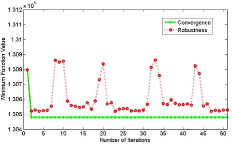
Fig. 1. Convergence and robustness.
This is an ODRAP. ByProposition 3, a PODRAP is obtained by adding the missing constraints
∑
21i=1Vi
(
ui24+ · · · +
ui2+
ui1)
≤
Rmax−
R1+
(
D1+
D2+· · ·+
D24)
. For this PODRAP, MPCAlgorithm 1converges to the global minimum 1
.
3048×
105of VLS(
0,
24]
at thesecond loop (see the solid line inFig. 1). As for the robustness of the MPC algorithm, assume thatuopt
[
k|
k]
in Step (2) ofAlgorithm 1isreplaced byuopt
[
k|
k] +
w
[
k]
, wherew
[
k]
is a noise vector and eachof its components is generated randomly by the Matlab uniform distribution function rand
(
1)/
50. The minimum objective function value varies within a small neighborhood of the global minimum value 1.
3048×
105as is clear from the dotted line inFig. 1. If thefirst iteration step is excluded, thenFig. 1shows that the maximum error happens at the 8-th step. The relative error of 0.29% is quite satisfactory.
5. Conclusions
This paper introduces the perfect optimal dynamic resource allocation problem and provides a corresponding MPC algorithm to solve the periodic implementation problem for the optimal solution. The convergence and robustness of the MPC algorithm are proved. This establishes a close connection of an MPC solution and a solution of a global optimization problem. An application of the MPC approach to the voluntary load shedding problem for a water pumping system illustrates the convergence and robustness of this MPC algorithm.
Acknowledgements
We would like to thank the anonymous reviewers for their valuable comments, and Mrs. Mathilda du Preez for text editing this paper.
References
Aissi, H., Bazgan, C., & Vanderpooten, D. (2009). Min–max and min–max regret versions of combinatorial optimization problems: a survey.European Journal of Operational Research,197(2), 427–438.
Allgöwer, F., & Zheng, A. (2000). Nonlinear model predictive control. Berlin: Birkhauser Verlag.
Bazaraa, M. S., Sherali, H. D., & Shetty, C. M. (1993).Nonlinear programming theory and algorithms. New York: John Wiley & Sons.
Belfares, L., Klibi, W., Lo, N., & Guitouni, A. (2007). Multi-objectives Tabu search based algorithm for progressive resource allocation. European Journal of Operational Research,177, 1779–1799.
Biegler, L. T., & Zavala, V. M. (2009). Large-scale nonlinear programming using IPOPT: an integrating framework for enterprise-wide dynamic optimization. Computers and Chemical Engineering,33, 575–582.
Chang, T. S., & Seborg, D. E. (1983). A linear programming approach to multivariable feedback control with inequality constraints.International Journal of Control,37, 583–597.
Ferrari-Trecate, G., Gallestey, E., Letizia, P., Spedicato, M., Morari, M., & Antoine, M. (2004). Modeling and control of co-generation power plants: a hybrid system approach.IEEE Transactions on Control Systems Technology,12, 694–705. Garcia, C. E., Prett, D. M., & Morari, M. (1989). Model predictive control: theory and
practice—a survey.Automatica,25(3), 335–348.
Ibaraki, T., & Katoh, N. (1988).Resource allocation problems: algorithmic approaches. Cambridge: The MIT Press.
Lee, S., Kumara, S., & Gautam, N. (2007). Efficient scheduling algorithm for component-based network. Future Generation Computer Systems, 23, 558–568.
Lee, J. H., & Lee, J. M. (2006). Approximate dynamic programming based approach to process control and scheduling.Computers and Chemical Engineering,30, 1603–1618.
Middelberg, A., Zhang, J., & Xia, X. (2009). An optimal control model for load shifting-with application in the energy management of a colliery.Applied Energy,86, 1266–1273.
Munawar, S. A., & Gudi, R. D. (2005). A multilevel, control-theoretic framework for integration of planning, scheduling, and rescheduling.Industrial & Engineering Chemistry Research,44, 4001–4021.
Pasadyn, A. J., Lee, H., & Edgar, T. F. (2008). Scheduling semiconductor manufacturing processes to enhance system identification. Journal of Process Control, 18, 946–953.
Patriksson, M. (2008). A survey on the continuous nonlinear resource allocation problem.European Journal of Operational Research,185, 1–46.
Qin, S. J., & Badgwell, T. A. (2003). A survey of industrial model predictive control technology.Control Engineering Practice,11, 733–764.
Schrijver, A. (1998).Theory of linear and integer programming. New York: John Wiley & Sons.
van Staden, A. J., Zhang, J., & Xia, X. (2009). A model predictive control strategy for load shifting in a water pumping scheme with maximum demand charges. In IEEE Bucharest PowerTech.
Xia, X., Zhang, J., & Elaiw, A. (2009). A model predictive control approach to dynamic economic dispatch problem. InIEEE Bucharest PowerTech.
Zadeh, L. A., & Whalen, B. H. (1962). On optimal control and linear programming. IRE Transactions on Automatic Control,7(4), 45–46.
Zafra-Cabeza, A., Ridao, M. A., & Camacho, E. F. (2008). Using a risk-based approach to project scheduling: a case illustration from semiconductor manufacturing. European Journal of Operational Research,190, 708–723.
Zhang, J., Xia, X., & Alexander, D. (2008). Demand side optimal strategy for voluntary load shedding. In The second IASTED Africa conference on power and energy systems.
Jiangfeng Zhangobtained his B.Sc. and Ph.D. in computing mathematics from Xi’an Jiaotong University, China, in July 1995 and December 1999 respectively. From February 2000 to August 2002 he was a lecturer at the Shanghai Jiaotong University, China. Then he was a postdoctoral researcher in the Chinese University of Hong Kong, Ecole Centrale de Nantes (France), Nanyang Technological University (Singapore), University of Liverpool (UK), and University of Pretoria (RSA). He has been a senior lecturer and then an associate professor in the University of Pretoria from November 2008. He is a certified energy manager and a certified measurement and verification professional. His current research interests are energy management and control theory.