Performance-based control system design automation via evolutionary computing

PERFORMANCE-BASED CONTROL SYSTEM

DESIGN AUTOMATION VIA EVOLUTIONARY COMPUTING

K. C. Tan

and Y. Li

† Department of Electrical Engineering National University of Singapore

10 Kent Ridge Crescent, Singapore 119260.

E-mail: [email protected]

Centre for Systems and Control, and

Dept. of Electronics & Electrical Engineering Univ. of Glasgow, Glasgow G12 8LT, UK.

E-mail: [email protected]

I. INTRODUCTION

Over the past few decades there have been great advances in the development of linear control theories and algorithms, ranging from classical proportional plus integral plus derivative (PID), phase lead/lag and pole-placement to more sophisticated optimal, adaptive and modern robust control. Each of these schemes, however, has its own control characteristic or design strategy to tackle a specific class of control problems. For example, a controller designed from the LQR scheme tends to offer a minimized quadratic error with some minimal control effort to overcome actuator saturation, while an

H∞ controller offers robust performance with a minimal mixed sensitivity function to maintain system response and error signals within pre-specified tolerances despite uncertainties. With so many mutually independent schemes available to control engineers, however, an increasing challenge has been imposed to the engineers to select an appropriate control law that best suits the application on hand, and to determine the best controller structure with an optimal parameter set that best meets the performance requirements before any practical implementations are attempted [1-4].

Developing an ULTIC control system, however, involves simultaneously determining multiple coefficients by optimizing a performance index in a usually noisy and discontinuous multi-modal cost surface. Complexity, nonlinearity and constraints in practical systems, such as voltage/current limits, saturation, noise and disturbance, make the design problem difficult to solve by conventional analytical or numerical means [4-6]. Moreover, the index that reflects practical specifications may not be “well-behaved” and conventional search may only lead to local optimum in the modal multi-dimensional space [5-7]. Although existing modern design succeeds in solving certain class of control problems with derived analytical solutions, these methods only confined to a narrow domain with known limitations such as numerically or physically ill-posed problems, and difficult to take into account the usual hard constraints exist in practical systems [4,8,9]. Such a controller may lead to system degradation or may not realize the full potential of the controller when on-line implementation is performed. Therefore it is difficult to employ conventional methods to achieve a computer-automated design that provides highest possible performance and best meets the customer design specifications automatically.

algorithm is naturally suited for ULTIC system design optimization. The EA has been successfully applied to various control applications such as the PID controller design [12,13], pole placement adaptive control [14], linear control [15], optimal control [16,17], nonlinear and sliding mode control [18,19], robust stability [20], fuzzy logic control [21] and neural networks [22,23].

The issues of ULTIC design strategy and its problem formulation in both the frequency and time domain is presented in Section II. Section III illustrates a powerful evolutionary algorithm and its parallelism to achieve design automation of an ULTIC system. Apart from using a model, Section IV shows that the design can equivalently be achieved based on plant input-output (I/O) data directly, bypassing the system identification or linearization stage as required by usual control schemes. In Section V, the applicability of the ULTIC design is demonstrated and implemented on two physical plants, including a multi-input multi-output nonlinear coupled liquid-level system. Finally, conclusions are drawn in Section VI.

II. UNIFICATION OF LTI CONTROL LAWS

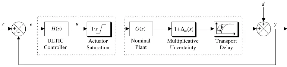
Therefore, a step towards unification of LTI controllers is to coin the design by meeting practical performance requirements, instead of by a specific scheme, or in a particular domain. Thus, a universal LTI controller as shown in Fig. 1 can be described by

0 1 0 1 ) ( ) ( ) ( b s b s b a s a s a s E s U s H n n n n + + + + + + = = L L (1)

where ai, bi ∈ ℜ+ ∀ i ∈ {0, 1, ..., n} are the coefficients to be determined in the design to satisfy certain specifications; L -1[E(s)] = e(t) is the error input to the controller, the amplitude of which may be restricted by an A/D converter; L -1[U(s)] = u(t) is the controller output voltage with a hard constraint saturation range such as the limited drive voltage or current. In Fig. 1, the plant G(s) to be controlled undergoes a number of perturbations including system time delays, multiplicative perturbations ∆m(s) and external disturbance d exist in most practical systems.

H(s) 1/s G(s) ₁+∆_{m( )s}

d y Transport Delay Multiplicative Uncertainty Nominal Plant Actuator Saturation ULTIC Controller e u r

Fig. 1 A practical unity negative feedback control system

The following formalizes the design issue and to develop an evolutionary computation based auto-mated design methodology. The feasibility of unifying classical and modern LTI control strategies in both the time and the frequency domains is reinforced, guided by performance satisfactions. The un-derlying aim is to let a practicing engineer conveniently to obtain an “off-the-computer” controller directly from customer specifications such as,

Spec. 1: A good relative stability of the closed-loop system (e.g. gain-margin ∈ [4 dB, 6 dB],

phase-margin ∈ [40 º, 60 º] or 3 dB bandwidth ≤ 10 Hz etc.);

Spec. 3: An excellent transient response in terms of small rise-time, settling-time, overshoots and undershoots (e.g. overshoots < 10 %);

Spec. 4: Robustness in terms of disturbance rejection; and

Spec. 5: Robustness in terms of plant uncertainties.

In order to satisfy various performance requirements, it is necessary to formulate different building blocks in an ULTIC design methodology. Since discontinuous performance index is allowed in evolutionary optimization, other specifications such as noise rejection, economical consideration and etc., may also be added if so desired. These individual building blocks could be added or multiplied to form a composite performance index by either arithmetic or logic operations if specific terms need to be emphasized, which offers an unmatched flexibility over conventional gradient-guided search methods.

A. Basic Performance Index for EA Guidance

In a design exercise, the closed-loop performance can be inverse-indexed conveniently by a basic cost function

) ( )

(

min H N e t

J = (2)

or

) ( ) ( 1

1 )

( ) (

min ω _{ω ω}

j G j H S

j E H J

+ = =

= (3)

Here N is the number of samples used for the simulation and S is known as the sensitivity function. The design task for basic performance is thus to find an optimal coefficient set of H(s) or {ai, bi} in (1)

such that Jmin(H) is minimized.

either the continuous time or the discrete time. The discussions here, however, are restricted in deterministic systems for simplicity, since the ULTIC strategy will be applicable to stochastic systems by involving an expectation operator in the cost function blocks. If the open-loop system is stable, then the Nyquist plot of the denominator of (3) should not encircle its origin in any way. This means that for relatively large stability margins, the denominator plot should be relatively far away from its origin and its magnitude should have a relatively large value. Hence, minimizing the basic index indirectly leads to robust stability and hence largely meets Spec. 1.

B. Reconciling Accuracy and Chattering

It is known that smooth control actions often lead to steady-state errors. High control actions usually result in low steady-state errors and high robustness, but also result in chattering and excessive wear of actuators. This may be reconciled by constructing performance index blocks in a similar manner to phase lag-lead compensation or PID control, noting that the chattering is reflected by e&, i.e., the rate of change of error. Note that index block manipulations can be easily realized in evolutionary guidance, since the EA only requires to compute Jmin and not its gradients. To penalize both the error and chattering at the steady-state in the time domain, weighting can be simply realized by multiplying the basic index by simulation time index. Also, weighting this way will not penalize a rapid transient response.

Therefore, the requirements of a high accuracy and low chattering at the steady-state to meet Spec. 2 and Spec. 3 can be reconciled in the time domain by adding to the basic index a building block of error derivatives and multiplying them by a building block of time as in

[

]

J

N

t

t t

∑

+ =

1

min & (4)

The magnitude of the transfer from the disturbance to the closed-loop output is give by

) ( ) ( 1

1 )

( ) (

ω ω ω

ω

j G j H j

D j Y

+

= (5)

Therefore, the disturbance rejection is maximized if the basic index or the sensitivity function S is minimized, which largely dealt with Spec. 4. In (5), the upper limit of this disturbance rejection is however bounded by the limited control gain due to the actuator saturation. To reflect the level of disturbance attenuation, the following performance weighting function is employed

σ( (S jω))≤W₁−1(jω) (6)

where σ defines the largest singular value and W₁−1(jω) is the desired disturbance attenuation factor.

Allowing W j1( ω) to depend on frequency ω enables one to specify a different attenuation factor for

each ω in the low frequency.

D. Robustness against Plant Uncertainty

Suppose the nominal plant in Fig. 1 is stable with ∆M being zero, then according to Small Gain

Theorem [24], the size of the smallest stable ∆M(s) for which the system becomes unstable is

)) ( (

1 ))

( (

ω σ ω σ

j T j

M =

∆ (7)

where T = GH

(

)

σ( (T jω))≤ W2− (jω)

1

(8)

where W2 j

1

−

( ω) is the respective sizes of the largest anticipated multiplicative plant uncertainties for the high frequency.

III. EVOLUTION ENABLES AUTOMATION

As addressed in the Introduction, evolutionary algorithm is probabilistic in nature and based on a

-posteriori information obtained by computerized trial-and-error, require no direct guidance and thus

no stringent conditions on the cost function. Supported by Schema Theory [25], EA requires an exponentially reduced search time, which could be further speeded up several times if engineers’ existing experiences are included in the initial design ‘database’ for intelligent design-reuse [26]. It is thus particularly useful to provide automated solutions for ULTIC design by incorporating different performance blocks in the optimization as to best meets the need of engineers’ design specifications.

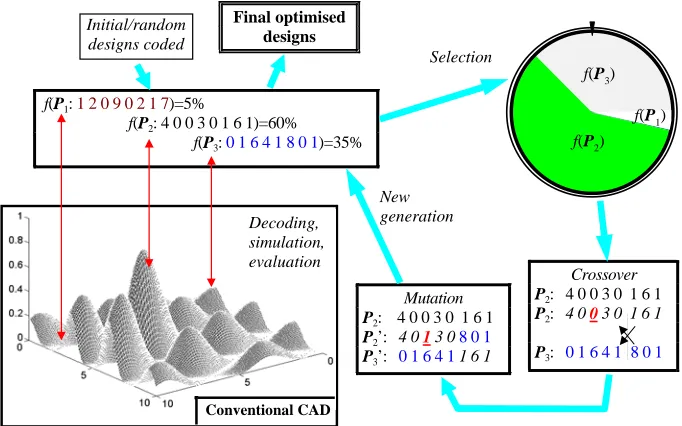
As illustrated in Fig. 2, conventional “computer-aided control system design” (CACSD) package that provides simulation results is used to evaluate performances of candidate controllers in terms of plant outputs, closed-loop errors and control signal provision. Artificial evolution then enables CACSD to become “computer-automated control system design” [4], where the performances on how well the candidate controllers meet the specification are used “intelligently” to guide the coefficient adjustment. This, however, requires a model of the plant to be controlled in the evaluation process.

Crossover

P2: 4 0 0 3 0 1 6 1

P2: 4 0 0 3 0 1 6 1

P3: 0 1 6 4 1 8 0 1

Mutation

P2: 4 0 0 3 0 1 6 1 P2’: 4 0 1 3 08 0 1 P3’: 0 1 6 4 11 6 1

f(P1: 1 2 0 9 0 2 1 7)=5%

f(P2: 4 0 0 3 0 1 6 1)=60%

f(P3: 0 1 6 4 1 8 0 1)=35% f(P2)

f(P₃)

f(P₁)

Conventional CAD

Decoding, simulation, evaluation Initial/random

designs coded

Final optimised designs

Selection

New generation

Fig. 2 Evolution automated CACSD by performance evaluations

IV. DIRECT DESIGN FROM PLANT STEP RESPONSE DATA

A. I/O Data Represent a High-Fidelity Model

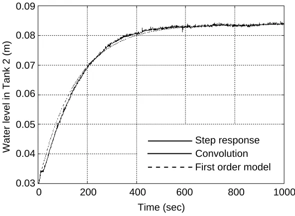
In many applications, step response data are often obtained when testing or setting the operating point of the system. An LTI model of the plant is then identified or refined from the I/O data before the design of a controller is attempted. An example of plant response data, ys(t), to a step input of

Ds e s K s G − + = τ 1 )

( (9)

with K = 0.018, D = 1 s and τ = 150 s.

Step response Convolution First order model

Water level in Tank 2 (m)

0.09 0.08 0.07 0.06 0.05 0.04 0.03 Time (sec)

0 200 400 600 800 1000

Fig. 3 Plant response data ys(t) for 3 V input, response of the first-order model and response obtained

by convoluting the impulse response

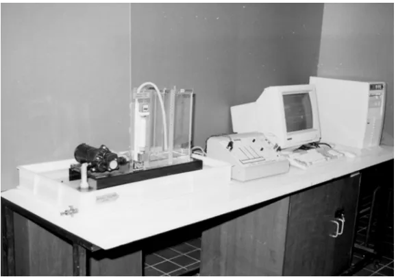
Owing to the simplicity and an acceptable accuracy, in certain control engineering practice, such a linear identification technique is even employed to fit data from a plant that may be internally nonlinear. Partly, this is because many nonlinear plants exhibit the “Type 0” behavior of an equivalent linear system, where all energy storing elements are causal and thus a non-zero control energy is needed to maintain the steady-state operating point as indicated by Fig. 3. It is interesting to note that the step response data were, in fact, obtained from the output y(t) of a nonlinear coupled liquid-level system as shown in Fig. 4. The system simulates the mass-balance dynamics usually found in the chemical and dairy plants with the nonlinear dynamics given by

Here the tanks are linked through a coupling pipe of an equivalent orifice area a1; the equivalent discharging area of Tank 2 is modeled by a2; the liquid level in Tank 1 is h1; thatin Tank 2 is h2with a physical constraint being h2 > H3, the equivalent height of both the coupling and discharging pipes; C1 and C2 are equivalent discharge constants; A = 0.01 m2 is the cross-sectional area of both tanks (which can be physically measured with a relatively high accuracy); Q1 and Q2 arethe input flow rate per actuating volt of the Tank 1 and Tank 2 respectively; and g = 9.81 m s-2 the gravitational constant.

Fig. 4 A nonlinear coupled liquid tank control system

Step response data of a plant represent a high fidelity infinite-order LTI “model”. Such a fidelity only holds at a consistent steady-state operating point if the plant is nonlinear. This opens a way of designing LTI controllers directly from plant step response data [4,29]. Of course, a more stimulating input whose spectra covers the plant bandwidth should reflect the dynamics of a practical plant more accurately. Note that this “modeling” approach may also apply to nonlinear plants for a given operating point, although a more accurate I/O relationship would be obtained by using the steady-state equilibrium and perturbing the plant round this point as adopted in linearization techniques [4]. This has eliminated the need of system identification or modeling process as required in most conventional control schemes.

B. Design Evaluation Based on Plant Step Response Data

Study Fig. 1 again, the closed-loop output contributed purely by the controlled input is given by

[

]

In Laplace or Fourier transform terms, this output can be evaluated by

) ( ) ( ) ( 1 ) ( ) ( ) ( ω ω ω ω ω

ω R j

j G j H j G j H j Y ⋅ +

= (12)

where A j Y j j

G( ω)= ω s( ω)

(13)

V ULTIC DESIGN EXAMPLES

A. ULTIC Design for a Linear Plant Directly from Open-Loop Response Data

Without loss of generality, a typical ODE defining the time-delayed DC servomotor system for velocity control is experimented in this paper. The servo-system is given by

) ( ) 06 . ( ) 06 . ( ) 06 .

( u t

LJ K t LJ RB t LJ LB JR

t T ⎟

⎠ ⎞ ⎜ ⎝ ⎛ = − ⎟ ⎠ ⎞ ⎜ ⎝ ⎛ + − ⎟ ⎠ ⎞ ⎜ ⎝ ⎛ + +

− ω ω

ω_{&& &} (14)

where u(t) ∈ [-5V, 5V] is the input field control voltage to reflect the saturation constraint of A/D converter; ω(t) ∈ℜ the angular velocity calculated from a Gray-code shaft encoder; KT = 13.5 NmA-1 the torque constant for a fixed armature current; R = 9.2 W the resistance of the field winding; B = 2.342 × 103 Nms the friction coefficient of the shaft; L = 0.25 H the inductance; and J = 0.001 kgm2 the moment of inertia of the motor shaft and load.

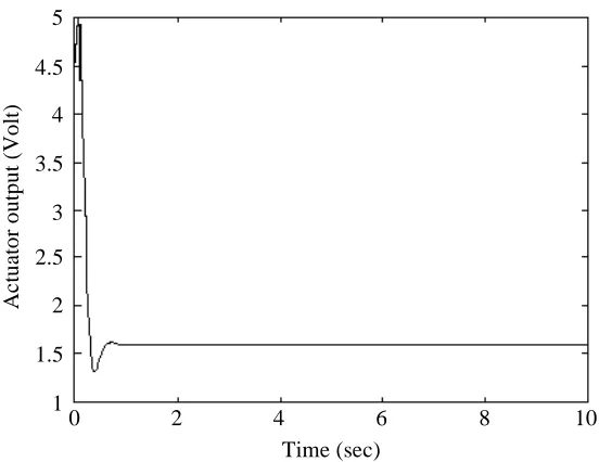
The design objective is to achieve a good closed-loop performance with excellent transient response and low chattering at the steady-state. For this, a limiting voltage of 5 V for the time-domain design or a penalized cost of 5−max(u) for the frequency-domain is incorporated with the performance index of (4) to limit the controller output drives within the saturation range, as well as to satisfy the various design criterion. The order of all candidate controllers is not fixed, while allowing its maximum to be third-order. Here a sampling period of 10 ms is used, as the time constant for this system is relatively small. The ULTIC controller of a minimal cost of (4) evolved directly from the step response data obtained from the physical system of (14) is given as

0 . 0 2 . 29 6 . 27 0 . 1 8 . 293 9 . 426 2 . 153 2 . 7 )

( _{3 2}

2 3 + + + + + + = s s s s s s s

H (15)

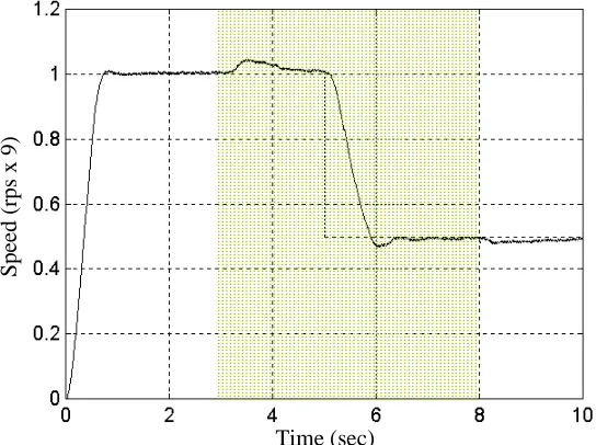
steady-state errors. The EA also tends to approach a 2nd-order controller for this 2nd-order plant, as the coefficients a3 and b3 are relatively small. If the order of the controller is restricted to the 2nd-order, however, it will result in a high gain controller [5]. In order to test the EA designed controller, a reference given by

r(t) = 2Bu(t) - Bu(t-τ) r.p.s. (16) is applied, where B = 4.5, u(t) is the unit step signal, and τ = 5 s. The eddy current brake of the system is released at t = 3 s and reapplied at t = 8 s, to test the system robustness in tolerating any plant perturbations or friction disturbance. The captured closed-loop response of this system is shown in Fig. 5, which confirms that the ULTIC approach yielded a excellent transient and steady-state performance, with good robustness against the plant uncertainties.

Sp

eed (rps x 9)

Time (sec)

Fig. 5 Implemented performance of the I/O data evolved ULTIC system, where plant uncertainties occur at the boundaries of the shaded area

B. ULTIC Design with Emphasis on Robust Performance

uncertainties and disturbances. For this, the weighting functions W1 and W2 are chosen to reflect the system performance and stability robustness as given by [3,4],

1 1

1 = ₊

s W 10000 ) 200 ( 50 2 + + = s s

W (17)

Stability verification is carried out for every candidate controllers, such that any designs with unstable poles on the right s-plane will be assigned a predefined high cost, without performing the closed-loop simulation to reduce the overall computation time. The resulting ULTIC controller is

s s s s s s S H 32 . 3 56 . 3 78 . 2 68 . 27 5 . 44 44 . 38 46 . 12 )

( _{3 2}

2 3 + + + + +

= (18)

Again, the EA tends to provide a controller that introduces an integrator to the Type 0 system of (14). The closed-loop response of this system for a step input of 60 r.p.m. (after a 9:1 step-down gear-box) is shown by Curve 1 in Fig. 6. To validate the robustness of the controller, a 0.2 Hz sine wave disturbance with peak-to-peak amplitude of 0.2 and 10 ms sampling period as shown by Curve 2 of Fig. 6 was applied to the system. The attenuated disturbance at the system output and the response of the motor system that suffered from this disturbance is shown by Curve 3 and Curve 4 in Fig. 6, respectively. The excellent performance clearly reveals that the specification of disturbance attenuation for the DC servo-mechanism has been met.

0 2 4 6 8 10 Time (sec)

1.2

1

0.8

0.6

0.4

0.2

0

-0.2

S

p

e

e

d

(

rms x 9)

2

4 1

3

3 4

Fig. 6 Response of the step and disturbance inputs

0 2 4 6 8 10 5

4.5 4 3.5 3 2.5 2 1.5 1

Time (sec)

A

c

tuat

or ou

tput

(V

ol

t)

Fig. 7 Controller output with an actuator constraint of 5 volt

C. Near-Linear Pipelinability and NP of the EA

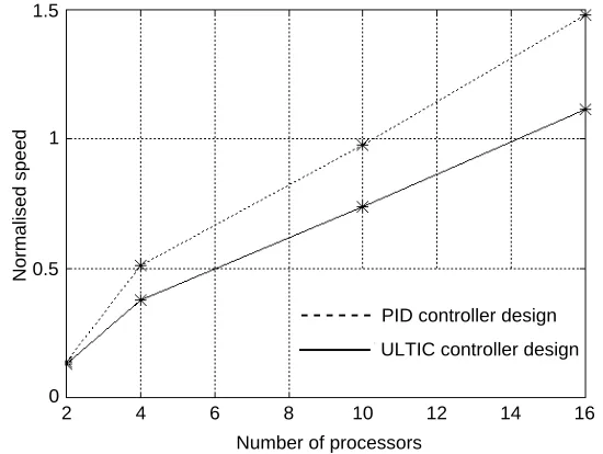
naturally suitable for parallel processing. The other advantage of the EA approach is the non-deterministic polynomial (NP) feature, which implies that designing a more sophisticated controller would not necessarily take more time than designing a simple one. To confirm this, the design of a three-coefficient pure PID digital controller has been repeated on the same numbers of transputers. The speedup is also plotted in Fig. 8. It can be inferred that, although the number of coefficients of the third-order controller is more than doubled, it only requires an O(n) = n× 25% increase in the design time, mainly due to the increased simulation time for the more complicated controller.

PID controller design

ULTIC controller design

16 14 12

10 8

6 4

Number of processors 1.5

0 0.5 1

2

Normalised speed

Fig. 8 The near-linear pipelinability and NP feature of the parallel EA

D. ULTIC Design for a Nonlinear Plant Directly from Open-Loop Response Data

The pumped inflow Q1 is the input used to control the liquid level in Tank 2. Here, the inflow Q2 is used as a disturbance into Tank 2 and is given by

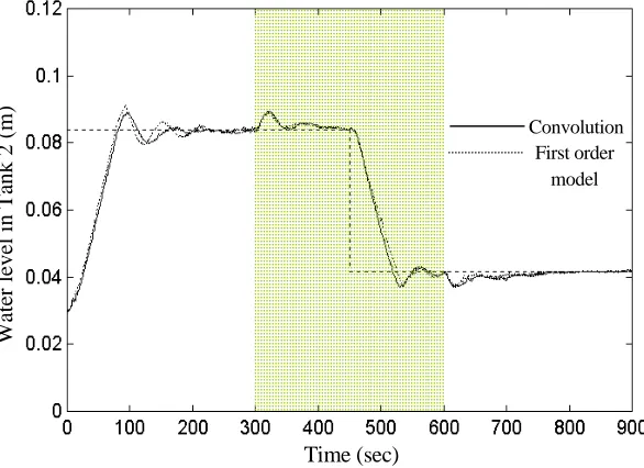
Q2(t)= 8.33 [u(t-300)- u(t-600)] cm3s-1 (19) The ULTIC controller designed from the EA is given by

0 . 0 44 . 0 82 . 1 0 . 1 73 . 1 273 151 243 )

( _{3 2}

2 3 + + + + + + = s s s s s s s

H (20)

It is seen that the EA tends to supply an integrator to the Type 0 system of (10) to eliminate the steady-state error. To compare with the model-based approach, another third-order controller was designed from the identified first-order model given by (9). The resultant controller is

0 . 0 40 . 0 81 . 1 0 . 1 44 . 1 299 190 217 )

( _{3 2}

2 3 + + + + + + = s s s s s s s

H (21)

The performances of controlling the physical coupled liquid-level system by these two controllers have been tested upon two different operating levels and added disturbances. The closed-loop step responses of Fig. 9 clearly reveals that the ULTIC designed without a model had offered a slightly better performance in controlling the nonlinear system.

Time (sec)

Wat

er

level in T

ank 2

(m

) First order model

Convolution

Fig. 9 The implemented performances of the ULTIC controllers designed from the I/O data and the first-order model, where disturbance occur at t = 300 and 600 sec

E. ULTIC Design for a MIMO Nonlinear Plant

Convolution First order

Here, an MIMO configuration of the nonlinear couple liquid-level system of Fig. 4 is studied such that the water level of 10 cm for Tank 1 and 9 cm for Tank 2 are controlled with minimized rise-time, overshoots and steady-state errors. The input to Tank 2, Q2, is now the second system input. For this system, a diagonal controller would suffice [19], i.e., the controller has a transfer function matrix given by,

H =⎡

⎣ ⎢ ⎤ ⎦ ⎥ H H 1 2 0

0 (22)

Note that the steady-state value of liquid level in Tank 1 has to be specified higher than that of Tank 2 due to the requirement of outflow of liquid in Tank 1 through Tank 2 to reach the reservoir as described by (10). Moreover, the steady-state levels of Tank 1 and Tank 2 are bounded with a maximum difference of

h h Q C a g 1 2 1 1 1 2 2 ( )∞ − ( )∞ ≤ ⎛ ⎝ ⎜ ⎞ ⎠ ⎟ (23)

at the extreme of Q2 = 0 with a given Q1. Similarly,

(

)

h H

C a g h h

C a

g

2 3

1 1 1 2

2 2 2 2 2 ( ) ( ) ( ∞ − ≤ ∞ − ∞ ⎧ ⎨ ⎪ ⎩⎪ ⎫ ⎬ ⎪ ⎭⎪ (24)

A transport delay of 1 s is found in each I/O channel of the physical system and is included in the design simulation. The obtained best diagonal ULTIC transfer function elements are

H s s s s

s s s

1

3 2

3 2

7 9 3013 95 7 102

10 0 98 0 73 0 0

( ) . . . .

. . . .

= + + +

+ + + (25)

H s s s s

s s s

2

3 2

3 2

4 69 55 76 57 56 0 86

10 0 46 0 38 0 0

( ) . . . .

. . . .

= + + +

+ + + (26)

copes well with the presence of the ‘untrained’ operating point at the step-down level. Subject to the hard voltage limit, the control signal that provides this closed-loop response is given in Fig. 11.

Water level in Tank 1 Water level in Tank 2

Wa

te

r le

vel (

m

)

Time (sec)

Fig. 10 Performance of the implemented MIMO ULTIC system

T im e (se c )

C

o

ntro

l s

ign

al (V

olt)

VI. CONCLUSIONS

In this paper, a parallel evolutionary algorithm based technique has been developed for the design unification of linear control systems in both the time and the frequency domains under performance satisfactions. A speedup of near-linear pipelinability is observed for the EA parallelism implemented on a network of Parsytec SuperCluster transputers. It is shown that the design can be further automated by efficient evolution from plant step response data, bypassing the system identification or linearization stage as required by conventional designs. Using the evolutionary ULTIC approach, control engineers only need to feed the CACSD system with the plant I/O data and customer specifications to obtain an optimal “off-the-computer” controller. In addition, the resulting ULTIC systems are easy to implement with only minor storage and computational overheads. This ULTIC design strategy has been validated against linear and nonlinear plants, with excellent performances and good robustness in the presence of constraints and perturbations.

Further work of the ULTIC methodology includes the application of multi-objective evolutionary algorithms to allow control engineers to integrate and visualize the set of performance criteria [3,30], as well as to incorporate other design objectives such as mixed-norm, controller structures and economical costing considerations.

ACKNOWLEDGEMENT

REFERENCES

[1] Y. Li, K. C. Tan, K. C. Ng and D. J. Murray-Smith, “Performance based linear control system design by genetic evolution with simulated annealing,” Proc. 34th IEEE CDC, New Orleans, 731-7363, 1995.

[2] Y. Li, K. C. Tan and C. Marionneau, “Direct design of uniform LTI controllers from plant I/O data using a parallel evolutionary algorithm,” Int. Conf. on Control'96, Special Session on

Evolutionary Algorithms for Control Engineering, University of Exeter, UK, 680-686, 1996.

[3] K. C. Tan and Y. Li, “Multi-objective genetic algorithm based time and frequency domain design unification of control systems,” IFAC Int. Sym. on Artificial Intelligence in Real-Time

Control, Kuala Lumpur, Malaysia, 61-66, 1997.

[4] K. C. Tan, Evolutionary Methods for Modelling and Control of Linear and Nonlinear Systems. Ph.D. Thesis, Dept. of Electronics and Electrical Eng., University of Glasgow, UK, 1997.

[5] Y. Li, “Modern information technology for control systems design and implementation,” Proc.

2nd Asia-Pacific Conference on Control and Measurement, Chongqing, China, pp. 17-22, 1995.

[6] Y. Li,K.C.Ng, K. C. Tan, D. J. Murray-Smith, G. J. Gray, K. C. Sharman and E. W. McGookin, “Automation of linear and nonlinear control systems design by evolutionary computation,”

Proc. IFAC Youth Automation Conf., Beijing, China, pp. 53-58, 1995.

[7] A.J.Chipperfield and P. J. Fleming,“Gas turbine engine controller design using multiobjective genetic algorithms,” Proc. First IEE/IEEE Int. Conf. on GAs in Eng. Syst.: Innovations and

Appl., Univ. of Sheffield, 214-219, 1995.

[8] Y. Chiang and M. G. Safonov, Robust Control Toolbox. The MathWorks, Inc, 1992.

[10] Z. Michalewicz, Genetic algorithms + Data Structure = Evolutionary Programs. Springer-Verlag, Berlin, 2nd Edition, 1994.

[11] D. B. Fogel, Evolutionary Computation. IEEE Press, Piscataway, NJ, 1995.

[12] P. Wang and D. P. Kwok, “Auto-tuning of classical PID controllers using an advanced genetic algorithm,” Proc. 1992 Int. Conf. on Ind. Electronics, Contr., Instrumentation and Automation, vol. 3, pp. 1224-1229, 1992.

[13] D. P. Kwok and F. Sheng, “Genetic algorithm and simulated annealing for optimal robot arm PID control,” Proc. 1st IEEE Conf. on Evolutionary Computation, IEEE World Cong. on

Computational Intelligence, Orlando, FL, vol. 2, pp. 708-713, 1994.

[14] K. Kristinsson and G. A. Dumont, “System identification and control using genetic algorithms,”

IEEE Trans. Syst., Man and Cyber., vol. 22, no. 5, pp. 1033-1046, 1992.

[15] D. P. Kwok, P. Tam, Z. Q. Sun and P. Wang,“Design of optimal linear regulators with steady-state trajectory insensitivity,” Proc. IECON 91, vol. 3, pp. 2183-2187, 1991.

[16] K.J.Hunt,“Polynomial LQG and H∞ controller synthesis - A genetic algorithm solution,” Proc.

31st IEEE CDC, Tucson, AZ, vol. 4, pp. 3604-3609, 1992.

[17] K. J.Hunt, “Optimal controller synthesis: a genetic algorithm solution,”IEE Colloq.on Genetic

Algorithms for Contr. Sys. Eng. Digest, vol. 106, pp. 1/1-1/6, 1992.

[18] Y. Li, K. C. Ng, D. J. Murray-Smith, K. C. Sharman and G. J. Gray, “Genetic algorithm automated approach to design of sliding mode control systems,” Int. J. of Contr., vol. 63, no. 4, pp. 721-739, 1996.

[19] K. C. Ng, Switching Control Systems and Their Design Automation via Genetic Algorithms. Ph.D. Thesis, Dept. of Electronics and Electrical Eng., University of Glasgow, UK, 1995.

[21] C. L. Karr, “Design of an adaptive fuzzy logic controller using a genetic algorithm,” in Genetic

Algorithms:Proc. 4th Int. Conf. on Genetic Algorithms, R. Belew, Ed., San Mateo, CA: Morgan

Kaufman Publishers, pp. 450-457, 1991.

[22] S. A. Harp and T. Samad, “Optimizing neural networks with genetic algorithms,” Proc.

American Power Conf., Chicago IL, vol. 54,pp.1138-1143, 1992.

[23] Y. Li and A. Häußler, “Artificial evolution of neural networks and its application to feedback control,” Artificial Intelligence in Engineering, vol. 10, no. 2, pp. 143-152, 1996.

[24] G. Zames, “On the input-output stability of time-varying non-linear feedback systems,” Parts I and II, IEEE Trans. Auto. Control, AC-11, 2 & 3, 228-238 & 465-476, 1966.

[25] D. E. Goldberg, Genetic Algorithms in Search, Optimization and Machine Learning. Addision-Wesley, Reading, Masachusetts, 1989.

[26] K. J. MacCallum, et al., “Design reuse – Design concepts in new engineering contexts,” Proc.

Control, Design and Production Research Conf, Heriot-Watt Univ, 51-57, 1995.

[27] S. Gordon and D. Whitley, “Serial and parallel genetic algorithms as function optimizers,” Proc.

of the fifth Int. Conf. on Genetic Algorithms, San Mateo, pp. 177-183, 1993.

[28] K. J. Åström and E. Wittenmark, Adaptive Control. Addison-Wesley, Reading, MA, 1995. [29] W. R. Cluett and L. Wang, “Modelling and robust controller design using step response data,”

Chemical Eng. Science, vol. 56, pp. 2065-2077, 1991.

Listing of Figure Captions

Fig. 1 A practical unity negative feedback control system

Fig. 2 Evolution automated CACSD by performance evaluations

Fig. 3 Plant response data ys(t) for 3 V input, response of the first-order model and response obtained by convoluting the impulse response

Fig. 4 A nonlinear coupled liquid tank control system

Fig. 5 Implemented performance of the I/O data evolved ULTIC system, where plant uncertainties occur at the boundaries of the shaded area

Fig. 6 Response of the step and disturbance inputs

Fig. 7 Controller output with an actuator constraint of 5 volt

Fig. 8 The near-linear pipelinability and NP feature of the parallel EA

Fig. 9 The implemented performances of the ULTIC controllers designed from the I/O data and the first-order model, where disturbance occur at t = 300 and 600 sec

Fig. 10 Performance of the implemented MIMO ULTIC system