Localisation and Navigation: Applying
Biological Principles in Mobile Robotics
by
Robert Ollington, BSc. Hons.
Submitted in fulfilment of the requirements for the Degree of
Doctor of Philosophy
Declaration
This thesis contains no material which has been accepted for a degree or diploma by the University or any other institution, except by way of background information duly acknowledged in the thesis.
To the best of my knowledge and belief, no material previously published or written by another person is included, except where due acknowledgment is made in the text of the thesis.
Robert Ollington
11 January, 2007
-er
c:::;r:x
·
Qer:. a;;7· I--~
Ll.
c·-
.,
~
~
'
:
(. '
o
·
L' :
Abstract
Recently, there has been a significant effort to apply behavioural and anatomical studies ofhippocampal place learning in rodents and other animals to the problem of robot localisation and mapping. The stated purpose of these recent experiments is twofold. Firstly, it is hoped that a study of this material will lead to improved algorithms for mobile robotics. Secondly, the behaviour of these new algorithms may be studied to evaluate psychological theories, and aid in the development of new theories. This thesis builds on these experiments by developing a complete localisation and navigational system for a simulated mobile robot. In order to provide a complete and efficient system, several new algorithms were developed.
Firstly, a method for preprocessing input was required, thus the adaptive response function neuron (ARFN) was developed. This neuronal model is able to identify similar input patterns, while discriminating between conceptually different sensory experiences. ARFNs learn a locally tuned response to input patterns, and are able to adapt the centre, width and shape of each input's response function on-line. These cells demonstrate one simple way that neurons in the cerebral cortex may learn a locally tuned response to input.
Secondly, a place cell system was developed for localisation. The new system provides a simple technique for establishing place cell firing based on odometric information and the current view (as captured by ARFNs). This system enables the robot's position to be accurately estimated, even in the presence of random and systematic odometric errors. The main advantage of the new system is that it allows certain topological assumptions to be made a priori, thus accelE;rating the training of downstream navigational systems. This prior Rnowledge--In.ay help explain the dead reckoning abilities of some animals and provides new insights into the place cell system in general.
coordinate learning is not necessary to solve behavioural tasks previously thought to require an abstract vector representation.
Acknowledgments
I would like to thank Dr Peter V amplew for his support and advice throughout the project. He has been a great friend and supervisor. Thanks also to my associate supervisor, Dr Ray Williams, for filling in for Pete, providing an alternate viewpoint, and for extensive assistance with other duties.
For their support and encouragement over many years, I would like to thank my parents; I would never have got this far without their help. Thanks also to the rest of my family, especially my wife Nadia for her patience, encouragement and valuable assistance throughout my studies, and to Isabel and Nicholas for putting up with my grumpy moods.
I would also like to thank: Richard Dazeley, for valuable discussions throughout the project; Sungsik Park, for his support and comments; and the G&AI research group, especially Adam Berry and David Benda, for help and distractions in equal measure. In addition, the entire academic staff of the School of Computing have been very supportive throughout my degree. In particular, I would like to thank Dr Julian Dermoudy and Nicole Clarke for feigning interest in my research, and for assistance with teaching and other duties.
Contents
Declaration •••••••••••••••••••••••••••••••••••••••••••••••••••••••••••••••••••••••••••••••••••••••••••••••••••••••••••••••Ill
Abstract •••••••••••••••••••••••••••••••••••••••••••••••••••••••••••••••••••••••••••••••••••••••••••••••••o•••••••••••• Vil
Acknowledgments ... ix
Contents ••••••••••••••••••••••••••••••••••••••••••••••••••••••••••••••••••••••••••••••••••••••••••••••••••••••••••••••• XI Chapter 1. Introduction ... 1
1.1. Hypotheses ... 2
1.2. Methodology ... 3
1.3. Structure of the Thesis ... 3
Chapter 2. Localisation and Navigation in Nature ... 5
2.1. 2.2. 2.2.1. 2.2.2. 2.3. 2.4. 2.5. Cognitive Maps and the Hippo campus ... 6
Hippocampal Input: Head Direction and Local View ... 11
Head direction ... 12
Local View ... 15
Place Cell Learning: Path Integration and Localisation ... 16
Hippocampal Output: Path Planning and Goals ... 17
Summary ... 19
Chapter 3. Localisation and Navigation: Computational Models ... 21
3.1. 3.1.1. 3.1.2. 3.1.3. 3.1.4. 3.2. 3.2.1. 3.2.2. 3.2.3. 3.2.4. 3.3. Localisation and Mapping ... 21
Analysing the Local View: Extracting Landmarks ... 21
Generating Place Cells from the Local View ... 24
Path Integration ... 25
Kalman Filtering ... 27
Navigation ... 30
Coordinate Based Navigation ... 30
Potential Fields ... 31
Reinforcement Learning ... 3 2 Hierarchical Navigation ... 32
3.4. Summary ... 34
Chapter 4. System Design ... 35
4.1. Localisation ... 35
4.2. Navigation ... 38
4.3. Integration ... : ... 39
Chapter 5. View Cell System
···••&••···
415.1. 5.1.1. 5.1.2. 5.1.3. 5.1.4. 5.2. 5.3. Adaptive Response Function Neurons ... .42
The Neural Model ... 43
Training ... 45
Validating the Model: Classification ... 49
Summary ... 54
ARFNs as View Cells ... 54
Summary ... 60
Chapter 6. From View Cells to Place Cells ... 61
6.1. 6.1.1. 6.2. 6.3. Combining Path Integrator and View Cell Input.. ... 61
Place Fields ... 64
Correcting Odometric Errors ... 69
Summary ... 71
Chapter 7. Low-Level Navigation ... 73
7.1. 7.1.1. 7.1.2. 7.1.3. 7.1.4. 7.1.5. 7.2. 7.2.1. 7.2.2. 7.2.3. 7.2.4. 7.3. Temporal Difference Leaming ... 7 4 Actor-Critic ... 75
SARSA ... 76
Q-Leaming ... 77
Eligibility Traces ... 77
Function Approximation ... 81
Low-Level Design and Testing ... 83
Reward Structure ... 83
Exploration and Leaming Strategy ... 83
Input Representation ... 84
Testing ... 84
Summary ... 86
Chapter 8. High-Level Navigation ... 87
8.2. 8.2.1. 8.2.2. 8.2.3. 8.2.4. 8.2.5. 8.3.
Concurrent Q-Learning ... 89
Adding Eligibility Traces to CQL. ... 93
Using Q-Values for More Efficient Learning ... 95
CQL Performance in the Watermaze ... 97
CQL Performance in Dynamic Environments ... 102
Hierarchical Learning for Reducing the Complexity of CQL ... 104
Summary ... 114
Chapter 9. System Integration and Testing ...•.... 115
9.1. 9.1.1. 9.1.2. 9.1.3. 9.2. 9.2.1. 9.2.2. 9.3. Chapter 10. 10.1. 10.2. 10.3. 10.4. References Appendix A. Appendix B. Appendix C. Appendix D. Integration ... 115
Goal Memory ... 116
Planning Updates ... 118
Combining Planning and Low-Level Navigational Input.. ... 120
Pre-training and Initialisation ... 121
View Cells and Low-level Navigation ... 121
Place Cells and High-Level Navigation ... 122
The Complete System ... 126
Conclusion ... 133
Localisation ... 13 3 Navigation ... 134
Biological Implications ... 134
Future Work ... 136
. ... 139
Simulation ... 149
Symbols Used ... 153
View Dataset ... 157
Chapter 1. Introduction
Mobile robotics is an exciting field of study with applications m defence, exploration, accessibility, transportation and recreation. Mobile robots allow operations in areas that are unsafe, uninteresting or otherwise impractical for a direct human presence. Most of these applications require some level of autonomy. For example, a robot exploring the surface of Mars, cannot receive human guidance in real time and must be able to complete some tasks independently for efficient operation. Similarly, if a robot is required to perform a task that is considered uninteresting for a human operator, the robot must be able to act autonomously.
One key attribute required by mobile robots is the ability to localise and navigate within a potentially unfamiliar environment. While researchers have made dramatic improvements in this area in recent years, it is clearly evident that the navigational abilities of mobile robots are still easily outmatched by those of animals. It would seem apparent that a lot can be learned from studies of animal navigation. However, the study of such fundamental behaviour is not always easy.
Chomsky (1968, p24) stated that "one difficulty in the psychological sciences lies in the familiarity of the phenomena with which they deal". This statement is equally true for the field of artificial intelligence, a field closely associated with the psychological sciences. For abilities involving spatial cognition and navigation, this is especially true. Even simple questions such as "how do I know where I am?" can be very difficult to answer either informally or formally. Despite these difficulties, we are able to apply these cognitive abilities with ease to solve complex spatial problems.
new paths opened, the rats were able to choose the path that lead most directly to the goal location. Similar abilities have been documented for many other animal species, ranging from ants (Wehner & Raber, 1979) and bees (Dyer, 1996), to birds (Wiltschko, 1997) and other rodents (Alyan & Jander, 1994; Etienne, 1987; Mittelstaedt & Mittelstaedt, 1980).
In contrast to the ease with which animals are able to solve complex navigational tasks, traditional techniques in artificial intelligence have difficulty solving some problems that appear relatively simple. While this is most apparent for simple sensory processing, it is also true of higher cognitive processes such as spatial cognition. It is therefore important to gain a greater understanding of the biological mechanisms in order to develop improved artificial navigation algorithms. Conversely, Hirtle and Heidorn (1993) have stated that the development of a computational model may aid in the development of biological theories by focusing on the processes and representations involved.
The aim of this thesis is to develop an artificial navigation system based on studies of animal navigation and biology, with the goals of extending the range of tools available for use in mobile robotics, and to gain a better understanding of the biological systems. While this is not the first experimental work in this area, previous studies have focused mainly on localisation and mapping and have not explored the relationships between these systems and navigation. Here a holistic approach is taken covering localisation and both low level and high level navigational cognition.
1.1. Hypotheses
Given that animals display navigational abilities that clearly outmatch those of mobile robots, it was hypothesised that:
A study of past and recent psychological and anatomical studies may
lead to new navigational solutions that may be applied in the field of
mobile robotics. In particular, a navigational system developed in this
way should be able to deal gracefully with dynamic goals and
environments, and produce apparently natural behaviour in the face of
Furthermore, it was hypothesised that:
The implementation of a biologically inspired solution for localisation
and navigation may provide valuable new insights in the field of spatial cognition. This should be particularly true for interactions between the
localisation and navigational system, as this is an area that has not been
extensively studied
Finally, this research may have relevance to fields other than spatial cognition. The brain areas associated with localisation and navigation also play major, and presumably similar, roles in other cognitive tasks. Therefore, it should be possible to adapt algorithms based on these biological systems to more general problems in the field of artificial intelligence.
1.2. Methodology
To assess the validity of these hypotheses it was proposed that a complete navigational system, based on developments in the field of spatial cognition, be developed for a simulated mobile robot. While experiments conducted in simulation only will not provide a definitive verification of the proposed methods, there are many advantages of such an approach. Aside from time and cost, simulated experiments allow a range of environments and robot configurations to be tested quickly, and allow the researcher to concentrate on the algorithms rather than the hardware.
Given that in nature successful navigation is not reliant upon a well-developed visual system, it was decided to implement the system for a simulated robot with range, tactile, and odometric sensors only. A full description of the simulated robot and environment can be found in Appendix A.
In addition to this simulation, more simplistic problems were also considered in the development of some algorithms. For example, classification problems were used in Chapter 5, and grid-world problems were used extensively in Chapter 8.
1.3. Structure of the Thesis
Chapter 5 and Chapter 6 discuss the implementation of systems used for localisation. Chapter 7 discusses a system for low-level navigation, and in Chapter 8 a novel reinforcement learning algorithm for path planning is developed. Chapter 9 details the integration of these sub-systems and presents the results of testing in various . configurations and environments.
Chapter 2. Localisation and Navigation in
Nature
Animals and humans show a remarkable ability to navigate in complex environments with apparent ease. This ability can be broken down into a number of non-trivial sub-tasks. These tasks include:
Localisation. The ability to know one's current location and orientation with respect to the environment. While this ability may seem trivial, it is in fact a complex task requiring the interaction of many sensory systems.
Path Integration. Also known as dead reckoning, this ability allows an animal to track its progress as it moves around an environment. If an animal wishes to return to a previous location, path integration allows a direct route to be calculated. Path integration is also a critical component of localisation.
Mapping. Many navigational tasks require some form of spatial map to be learned and committed to memory. While some navigational tasks may be performed through a simple sensor/action association (taxon1 navigation), many tasks require a more abstract representation of ones environment.
Path Planning. Even with a map of the environment, path planning can be a difficult task in many environments. Furthermore, a robust path planning system should include the ability to find detours around novel obstructions, and to find shortcuts as these become available.
Goal Identification. While the identification of some goals may be quite straightforward, others can be more complex. Goal identification not only needs to identify important locations related to such primary needs as food and shelter, but also needs to address the issues of exploration and threat avoidance.
This chapter investigates some of the biological mechanisms that underlie these abilities. Section 2.1 introduces the concept of cognitive maps, and reviews evidence that the hippocampus may be the locus of this mapping ability and other aspects of spatial cognition. Section 2.2 examines information input to the
1
Taxon navigation is the term used to describe the group of navigational strategies based on simple
hippocampus and section 2.3 discusses some theories of how this input, along with a system for path integration, may provide a means for localisation. Section 2.4 presents new evidence suggesting that navigation and path planning may be achieved through reinforcement learning in the basal ganglia. Finally, the main points are summarised in section 2.5.
'
2.1. Cognitive Maps and the Hippocampus
Tolman (1948) proposed that the brain might hold a topological map of its environment, and that this map could be used for various navigational tasks. This cognitive map theory has also been strengthened by later experiments, such as those involving the Morris Watermaze (Morris, 1981; Steele & Morris, 1999).
The Morris Watermaze (Morris, 1981) is an example of a problem that cannot be solved without an abstract representation of space (Muller, Kubie, Bostock, Taube,
& Quirk, 1991). The Watermaze consists of a cylindrical environment filled with an
opaque liquid. A platform is placed just below the level of the liquid so that it cannot be seen by a swimming rat.
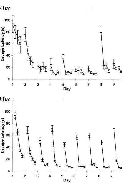
In the reference memory in the watermaze (RMW) task (Foster, Morris, & Dayan, 2000; Morris, 1981; Steele & Morris, 1999) rats are trained to find the location of the hidden platform over a period of several days, undergoing four trials per day. After this initial training period, the platform is moved to a new location. Once the new platform location is discovered, the rats are able to navigate directly to the new location on subsequent trials.
In the delayed matching-to-place (DMP) task (Foster et al., 2000; Steele & Morris, 1999) the platform is moved at the end of every day. Even in this more complex task, the rats are able to achieve "one-trial learning"2 after very few days. Typical results for the RMW and DMP tasks are shown in Figure 2.1.
a)120
100
-
U)->i 80
CJ
c
.e
_j
60Cl)
c.
~
40 U)w
20
b)120
100
-
U)->i 80
CJ
c
.e
_j
60Cl)
c.
~
40 U)w
20
1 2
1 2
3 4
5
6
7 8 9Day
3 4 5 6 7 8 9
Day
[image:19.562.87.486.60.658.2]Studies of brain lesions in animals (see Barnes, I988 for a review) and humans (Habib & Sirigu, I987) have identified the hippocampus as a possible location for the cognitive map proposed by Tolman. Figure 2.2 shows the hippocampus including some of the key neural connections. The hippocampus consists of two thin layers of neurons, called the dentate gyrus and Ammon's horn (cornu Ammonis,
abbrev. CA), that are folded over each other. Ammon's horn is divided into several groups of neurons of which only CAI and CA3 are relevant to this discussion. The hippocampus receives most input from the entorhinal cortex via a group of axons called the perforant path. Perforant path axons synapse on granule cells in the dentate gyrus, which in turn form connections with pyramid cells in CA3. CA3 neurons send output from the hippocampus via the fornix, to neurons in CAI via the Schaffer collateral, and also to a very large number of other CA3 neurons. CAI output also departs the hippocampus via the fornix, and the subiculum, which sends output back to the entorhinal cortex, thus completing a circuit.
CAI
[image:20.562.111.513.351.577.2]Fomix
Figure 2.2 The hippocampus, including some neural connections. Axons
O'Keefe and Dostrovsky (1971) observed that pyramid cells in the hippocampus of rats responded maximally when the rat was in a certain location. The region in the environment where a place cell, as these neurons are now known, fires most strongly is known as the cell's place field. The properties of place cells and place fields include:
• Place fields are established within about ten minutes of entering a new environment (Wilson & McNaughton, 1993).
• Place fields tend to follow local barriers within the environment. For example, Muller and Kubie (1987) found place fields in a cylindrical environment that extended along the wall of the cylinder, with the interior edges of these fields being concave.
• The combined output from a relatively small group of place cells is sufficient to accurately predict the rat's position to within a few centimetres (Wilson &
McNaughton, 1993). The combined output of all place cells is often referred to as the place code.
• Place fields are influenced by visual stimulus. If visible landmarks within an environment, are rotated, place fields rotate with respect to each other by the same amount (Muller & Kubie, 1987; O'Keefe & Speakman, 1987).
• In the absence of visual stimulus, place cells persist (Muller & Kubie, 1987; O'Keefe, 1976; O'Keefe & Speakman, 1987). Hence idiothetic information, such as vestibular, visual motion and motor efferent inputs, must also be able to influence place cell firing (Bures et al., 1999). Other experiments also confirm that path-integration or dead-reckoning is a crucial component of navigation in many animals (Alyan & Jander, 1994; Etienne, 1987; Mittelstaedt &
Mittelstaedt, 1980).
• Some place cells show correlations to non-spatial aspects of the environment, and it has been suggested that these cells may code for context with space being just one of the relevant parameters (Eichenbaum, 1996; Eichenbaum & Cohen, 1988; Eichenbaum, Otto, & Cohen, 1992; Markus et al., 1995; Muller & Kubie, 1987). For example, some cells show a correlation with the current behaviour of the rat.
• The proximity of place cells in the hippocampus bears no correspondence with the proximity of their place fields within the environment (Muller & Kubie, 1987; O'Keefe, 1976).
• Place fields in different environments are not correlated, and a cell exhibiting a place field in one environment may have no place field in another (Muller &
Kubie, 1987).
• Place cell firing actually predicts the future position of the rat on a short time-scale (~lOOms) (Muller & Kubie, 1989).
• Place cells have been found in other brain areas, but those in areas CAI and especially CA3, are most correlated with the rat's location (Amaral & Witter, 1989).
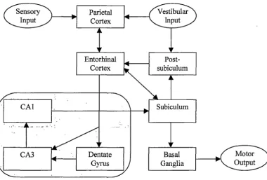
O'Keefe and Nadel (1978) suggested that these place cells might form the basis of a system for localisation and navigation. They proposed two different mechanisms; a "taxon" system, and a "locale" system. The taxon system was used for route learning. For a given route, each place cell would be associated with an appropriate response leading to the next location on the route. The locale system could be used for map-like navigation. The map was proposed to be an absolute Euclidean representation of the environment (O'Keefe, 1989, 1990, 1991). Such a representation would allow distances and directions to be calculated between the field centres of place cells.
Sensory Input
CAI
CA3
Parietal Cortex
Entorhinal Cortex
Dentate Gyrus
Post-subiculum
Basal Ganglia
[image:23.563.94.475.90.347.2]Motor Output
Figure 2.3 Some of the functional connections of the hippocampus and the place cell system.
2.2. Hippocampal Input: Head Direction and Local View
The major source of input to the hippocampus is the entorhinal cortex, and while some connections are made with areas CAI and CA3, the majority of this input is to the dentate gyrus. The entorhinal cortex receives highly processed sensory information originating in the parietal cortex (Deacon, Eichenbaum, Rosenberg, &
Eckmann, 1983), which receives sensory input including visual and vestibular input. The parietal cortex also receives feedback from the entorhinal cortex. The postsubiculum receives vestibular input and is a source of input to the entorhinal cortex. The subiculum is also a major source of input to the entorhinal cortex.
2.2.1. Head direction
Orientation and location are two interacting concepts necessary for absolute localisation3, with orientation being perhaps the simpler concept (Muller et al.,
1991). It seems sensible then, to examine the head direction system before attempting a detailed analysis of the place cell system.
Cells have been found in the postsubiculum that fire only when the rat's head is oriented in a particular direction. These head direction cells have many properties in common with place cells:
• The firing of head direction cells is independent of behaviour.
• The population of head direction cells provides an accurate, distributed representation for any head direction (Blair, Lipscomb, & Sharp, 1997).
• The firing of head direction cells is maintained even in total darkness (McNaughton, Chen, & Markus, 1991)
• Local landmarks influence the firing of head direction cells and may be used to correct errors in the head direction signal (McNaughton, Markus, Wilson, &
Knierim, 1993; Taube & Burton, 1995; Taube et al., 1990).
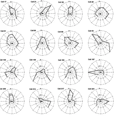
Other closely related brain areas also contain cells that clearly play an important role in maintaining the head direction signal. Neurons correlated with angular head velocity have been found in the dorsal tegmental nucleus (Basset & Taube, 2001 ), and in the anterior thalamus, head direction cells have been found that predict the rat's future head direction (Blair & Sharp, 1995). Head direction cells that fire more strongly when the rat is turning have been found in the lateral mamillary nucleus (Leonhard, Stackman, & Taube, 1996). Also of interest is the fact that the tuning curves (a plot of firing rate versus direction) of head direction cells are often distorted when the animal rotates as shown in Figure 2.4.
3
Absolute localisation is the ability to localise immediately upon entering an environment.
a)
60
'N e. "
1U 40
a:
.,,
c ·c u: 200
c)
Raw Data b) Gaussian Fit
60
40
20
0
0 60 120 180 240 300 360 0 60 120 180 240 300 360
Head Direction Head Direction
Turning Left d) Stationary e) Turning Right
M m W
=
300 360 0 M m W 360 0 60 120 180 300 360 [image:25.561.88.475.67.287.2]Head Direcl!on Head Direction Head D1rect1on
Figure 2.4: Head direction cell tuning curves. a) Typical raw data for the tuning curves of a uni-modal cell in the anterior thalamus. b) Tuning curves are normally approximated to a Gaussian fit. c ), d) and e) show idealised tuning curve distortion for an animal turning to the left and right for a cell with two tuning curve peaks. (adapted from Blair et al., 1997; Goodridge & Touretzky, 2000)
TMHDCells
n
(cnt) V
HD Cells
0
0
D
~·()
0
0 0
0
(>
O
Q
D~cens
0
0
0
(cnt)oOo
0
0
0
CJ
0
"
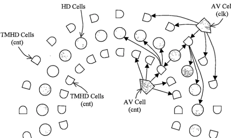
Figure 2.5: Model of the head direction circuit: showing head direction (HD), angular velocity (AV), tum-modulated head direction (TMHD) cells, and representative connections. Separate populations of AV and THMD cells are proposed for clockwise (elk) and counter-clockwise ( cnt) rotations. Each HD cell excites neighbouring TMHD cells, which in tum excite neighbouring HD cells in each direction. When the animal is not turning THMD input to HD cells is uniform in each direction, but when the animal turns AV cells increase the firing of corresponding THMD cell populations. This asymmetric input causes the activity of HD cells to shift in the appropriate direction. (adapted from Blair et al., 1997)
McNaughton and colleagues (1991) suggest that the integration of angular head velocity information is accomplished using a simple look-up table approach. Given the current head direction and the current angular velocity the conceptual table would store the unique head direction that would result after a certain time delta. The table would presumably be implemented via TMHD~HD cell connections.
[image:26.564.112.505.87.323.2]can be made to move in that direction. Through the choice of appropriate parameters, a network can be constructed that integrates angular velocity quite accurately.
A further refinement of the attractor hypothesis was developed that involved the coupling of two attractor networks representing cell populations in the anterior thalamus and postsubiculum respectively (Redish, Elga, & Touretzky, 1996). A similar model was later developed by Goodridge and Touretzky (2000) that also accounted for deformation of head direction tuning curves in the anterior thalamus (see Figure 2.4).
2.2.2. Local View
Place cells are strongly influenced by the local view, and it has been suggested that the source of this local view information is the entorhinal cortex (Redish &
Touretzky, 1997). The assertion that entorhinal cortex cells are directly associated with hippocampal place cells is strongly supported by the fact that the effects of cue rotation and removal on place cell firing is mirrored in the firing of entorhinal cortex cells.
The entorhinal cortex receives highly processed sensory information from neocortical areas, and entorhinal cortex 'place' cells are more influenced by sensory information than true place cells (Muller et al., 1991). Unlike place cells in CA3 and CAl, cells in the entorhinal cortex generally have 'place' fields in all environments (Muller et al., 1991), further supporting the notion that these cells may essentially form a coding for local view.
If entorhinal cortex cells do code for local view, then that view must be in allocentric 4 coordinates, since the firing of these cells is independent of the current head direction. In order to convert egocentric sensory information into an allocentric view, the entorhinal cortex must receive information about the current head direction. The entorhinal cortex does receive input from the postsubiculum and this input is likely to include head direction information, further supporting the local view hypothesis.
4
Strictly speaking, allocentric refers to an environment based reference frame, or world-centred
coordinates. However as in this case, it is often used to describe coordinates centred on the current
animal location but with orientations relative to the environment. Egocentric refers to an animal
Since place cells are more sensitive to changes in the local environment than to changes in distal landmarks (Muller & Kubie, 1987), it seems likely that any view cells influencing the firing of place cells will also be more sensitive to local cues. In particular, the distance to and orientation of nearby walls seems to have a particularly strong effect on place fields, and hence should be a major factor in view cell firing.
2.3. Place Cell Learning: Path Integration and Localisation
The main input to the hippocampus comes from the entorhinal cortex, and it has been proposed that the function of some entorhinal cortex cells is to identify local views. While hippocampal place cells are influenced by visual sensory cues, they also continue to fire in complete darkness, suggesting that local view cells are not the only influence on the firing of hippocampal place cells. In the absence of sensory cues, the only explanation is that the animal localises through some form of path integration or dead reckoning (McNaughton et al., 1991; Muller et al., 1991; O'Keefe, 1976). Evidence for path integration can be seen in the ability of a wide range of animals to return to a starting location after taking a circuitous route, even in total darkness (Alyan & Jander, 1994; Etienne, 1987; Mittelstaedt & Mittelstaedt, 1980). Furthermore, Sharp and colleagues (1995) report that hippocampal place cells are influenced by vestibular and visual motion inputs.
The functioning of the path integrator would be analogous to the head direction system described earlier. Input representing the perceived self-motion of the animal would move the centre of activity of the integrator cells. In this case, these would conceptually (but not necessarily physically) be arranged in a two-dimensional array. Input from local view cells would then allow corrections to be made to adjust for errors in the self-motion input.
It has been suggested that hippocampal place cells themselves form the basis of a path-integration system rather than a topological map (McNaughton et al., 1996). It is suggested that the ten minutes required for stable place fields to develop (Wilson
& McNaughton, 1993) would not be enough time for the formation of a consistent
place cells during sleep (Kudrimoti, McNaughton, Barnes, & Skaggs, 1995). The ability to make such a prediction suggests some degree of pre-configuration.
McNaughton and colleagues suggest this path integration system would operate in a similar way to their model for head direction integration (McNaughton et al., 1991). As with the head direction model, cells that are correlated with position and the direction of movement should have a direct influence on place cells. Cells in the subiculum satisfy this requirement but have only an indirect influence, via the entorhinal cortex, on place cells in the hippocampus. In support of this Redish and Touretzky (1997) propose that path integration is performed by a loop consisting of the hippocampus, subiculum and entorhinal cortex. In their model, local view and path integrator input is combined in the dentate gyrus, and these cells drive the place cells of CA3 and CAL If either the path integrator or local view input changes a different hippocampal place cell will be activated (Redish & Touretzky, 1999). Output from these place cells then feeds back to the path integration circuit via the subiculum.
In a similar way to the head direction system, path integration may be accomplished in part by an attractor network (Kali & Dayan, 2000). Recurrent connections between cells in CA3 could form the basis of a two-dimensional attractor network with a hill of activation representing the location of the animal in the environment. Applying appropriate self-motion related input could shift the hill of activation to facilitate path integration.
2.4. Hippocampal Output: Path Planning and Goals
stimulus
action 1 action 2 action 3
temporal representation
reward prediction error
reward
'--~~~~~ ~~~~~.)
y
[image:30.559.117.500.69.391.2]critic
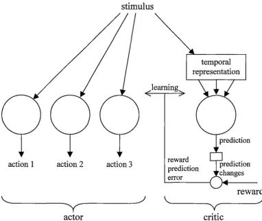
Figure 2.6: Neural implementation of actor-critic temporal difference learning. (adapted from Suri, 2002)
In Figure 2.6, the critic learns to predict the value of the current state, as represented by the input stimulus. The small circle in the figure represents dopamine neurons, which calculate the error in the predicted value. This error is then used to train the critic, and also the actor. The actor consists of discrete units corresponding to each possible action. The output of each of these actor units is a measure of the suitability of performing that action given the current stimulus. See section 7 .1 for a full description of temporal difference learning and the actor-critic architecture.
Another indicator that the basal ganglia are associated with reinforcement learning and navigation, arises from interactions with the hypothalamus. The hypothalamus is a centre for controlling motivational states (Swanson & Mogenson, 1981) and this motivational information is sent to, among other brain areas, the basal ganglia. Since satisfying many motivations will require moving to a particular location (e.g. moving to food), it seems likely that motivational signals would be sent to an area of the brain involved with navigation. This concept is explored further by Guazzelli, Arbib and colleagues (Arbib, 1999; Guazzelli, Corbacho, Bota, & Arbib, 1998) through their world graph theory. They propose a model for determining the rewards of an actor-critic learning algorithm by considering the current set of motivational drives. Neurons encoding the current motivational drives are assumed to reside in the hypothalamus, the output of these neurons then influences the firing of dopamine neurons in the basal ganglia.
Brown and Sharp (1995) developed what is essentially a reinforcement learning model of navigation by considering the interaction of place and head-direction cells, and motor neurons in the nucleus accumbens. In the model, the activity of place cells and head-direction cells result in the firing of cells in either of two groups of motor cells. One group corresponds to moving left and the other to moving right. A trace is kept of which group of cells fire for a given place and head-direction cell combination, and this trace decays over time. When the goal is encountered, synaptic connections between place and head-direction cells and motor neurons are strengthened according to the corresponding trace.
2.5. Summary
Chapter 3. Localisation and Navigation:
Computational Models
The field of mobile robotics is large and diverse. It would not be possible to review all of the research in the field relating to localisation, mapping and navigation, and furthermore much of this information would not be relevant to this thesis. The main aim of the thesis is to examine biological mechanisms that may be useful in the field of mobile robotics. Therefore, this chapter will review those computational models , that demonstrate applicability to mobile robotics and that claim some degree of
biological inspiration. In particular, those models inspired by the mammalian place cell system described in the previous chapter will be reviewed.
Section 3.1 will review models of localisation and mapping that attempt to simulate the place cell system itself. In section 3 .2, navigational models utilising a place cell representation will be discussed. Section 3 .4 will summarise this literature and discuss the strengths and weaknesses of experimental work to date.
3.1. Localisation and Mapping
3. 1. 1. Analysing the Local View: Extracting Landmarks
The first stage of localisation in biological systems is the activation of view-cells. Likewise, for all of the computational models reviewed, processing the current view formed an important first step in the localisation procedure.
Typically landmarks are first extracted from the local sensory view. The type, bearing, or range of each landmark (or some combination of these) is then either further processed or passed directly to the place cells. While this general principle is common for most of the syst~ms reviewed, they differ in the type of sensory information provided, the landmark information that is used, and the degree of further processing of this information.
In the simplest case, Guazzelli, Bota and Arbib (2001) conducted experiments in simulation only with the bearing and distance of three distal landmarks given directly to the agent.
Khepera5 mobile robot. The robot sensors consisted of video and short-range ( 4cm) infra-red proximity sensors. The environment was a rectangular 'room' with white walls and a dark floor. One wall had an identifying dark strip. As in the work of Gauzzelli and colleagues (2001 ), the range and bearing of landmarks, which in this case were the four walls of the environment, were used. The landmarks were found by rotating the robot to face each wall and acquiring an image. The image was then analysed to find the centroid of each wall, from which range and bearing information could be calculated.
Gaussier and colleagues (Gaussier, Joulain, Banquet, Lepretre, & Revel, 2000; Gaussier, Revel, Banquet, & Babeau, 2002) also extracted landmarks from camera images, however their system demonstrates that it is possible to extract useful landmarks in a more natural environment. The system was implemented on a Koala6 mobile robot equipped with a video camera capable of taking panoramic images over a 300 degree range. The robot operated in a 7.3m x 5.4m laboratory environment. Landmarks were extracted from the camera image using pattern recognition techniques. The image was first scanned for points of interest indicated by changes in horizontal image intensity. The area around these focal points was then compared to learned views. As with the two models discussed above, the bearing of each of these landmarks was extracted, but in contrast the type of landmark was used rather than the range.
Wan, Touretzky and Redish (Touretzky, Wan, & Redish, 1994; Wan, Touretzky, &
Redish, 1994a, 1994b) show that landmarks can also be extracted in real environments from more rudimentary sensory input. Their model was implemented on a Xavier7 mobile robot. This robot was equipped with a ring of 24 sonar sensors, an infrared laser rangefinder, and a colour camera. Information from the sonar sensors was stored in an occupancy grid8 and standard edge detection algorithms were used to detect comers. The locations and types (concave or convex) of these
5 Khepera is a small mobile robotics platform. See www.k-team.com for details.
6 Koala is a mid-sized mobile robotics platform. See www.k-team.com for details.
7 Xavier is another mid-sized robot. See www-2.cs.cmu.edu/~Xavier for details.
8 An occupancy grid, also called a free space map, divides the space into discrete cells and labels each
comers become the landmarks of the system. Ranges and bearings to these landmarks were used along with the angle of incidence between the landmarks.
The amount of further processing conducted on the extracted landmark information varies between researchers. Gaussier and colleagues (2000; 2002); and Wan, Touretzky and Redish (Touretzky et al., 1994; Wan et al., 1994a, 1994b) perform no additional processing, the raw landmark information is used directly as input to the place cells. The remaining models discussed in this section use the landmark information as input to a view cell layer where the information is refined before being sent to the place cell layer.
The view cells in the model of Burgess, Donnet and O'Keefe fired maximally when a particular wall was at a set distance from the robot. The output of the sensory cells was calculated using a Gaussian function, with the width of the Gaussian modified by the preferred distance of the wall, increasing as the preferred distance increases. Equation 3.1 gives the activation function for the ith sensory cell, where x is the distance from the wall, d1 is the cell's preferred direction, and A and a are tuning parameters.
---r==A=
exp [-( x -d,
)2 ]
~27rdd,
2dd,
3.1
Guazzelli, Bo ta and Arbib (2001) first form view cells that respond to the bearing and range of one particular landmark. A further layer of cells then receives input from a selection of the primary view cells corresponding to different landmarks.
view cells were then generated t~at depend on the activation of several simple view cells.
3. 1. 2. Generating Place,·Cells from the Local View
Burgess, Donnet and O'Keefe (1996; 1998) and Gaussier, Revel and Banquet (2000; 2002) each demonstrate that it is possible to generate simulated place cells that exhibit many of the properties of their biological equivalents from landmarks alone.
In the model of Burgess and colleagues (1996; 1998), the view cell output is sent to the next layer of cells, which model cells in the entorhinal cortex, via hard-wired connections. Each of these cells receives input from two view cells responding to two orthogonal walls. Output from this layer goes to the place cell layer; these on/off connections are trained using a form of competitive learning. Place cells then send output to goal cells, presumed to be in the subiculum. The structure of the model is shown in Figure 3.1.
w
Population Vector
~
NOsOEOwO
Goal Cells
Learning
0 0 0 0 0 0 0 0 0 0
Place Cells
Increasing Wall Distance
Q Q
Entorhinal Cells
[image:36.559.138.477.364.695.2]Sensory
Cells
Figure 3.1: The place cell model of Burgess, Donnet and O'Keefe (1996; 1998).
the environment is similarly distorted. However in a more complex environment, the robot would be subject to perceptual aliasing problems. That is, in environments where the vf~w from two distinct places may be identical or similar, place cells tuned to this view will not be able to distinguish between the two locales, and hence will have two place fields. This is not a desirable property if these place cells are to be used for navigation.
Place cells in the model of Gaussier and colleagues (2000; 2002) learn the expected bearings of visible landmarks when viewed from the corresponding environment location. The closer each landmark is to it's expected bearing, the higher the place cell activation. While this is potentially very useful, the resultant place fields do not resemble those of biological place cells. While the higher sensory resolution of the robot in this model would greatly reduce the risk of perceptual aliasing, it would nevertheless remain a problem with any view-only method.
3.1.3. Path Integration
Path integration alone is unable to produce a robust position estimate. Even if the system is perfectly accurate under normal circumstances, and this is almost impossible to achieve on a robotic platform, it is unable to provide initial localisation within the environment. Therefore, none of the models discussed in this chapter suggest a path integration only system for localisation. Instead, path integration is combined with the landmark or view cell information to overcome the perceptual aliasing problem.
Wan, Touretzky and Redish (Touretzky et al., 1994; Wan et al., 1994a, 1994b) combine the landmark information with current path estimate in a single step. The activation of place cells is determined using radial basis functions tuned to distances and bearings of landmarks, to the angles between landmarks, and to the path integrator coordinates. The expression for place cell activity is in the form of a product of Gaussians corresponding to each of these items. When any of this information is unavailable, the corresponding term drops out of the expression. This enables navigation in the dark and correct localisation when path integrator coordinates are known to be incorrect, such as when the robot enters the environment. For example, upon entering an environment, place cell activity is first calculated using the current view only. Each active place cell then recalls its learned position and orientation, and this information is used to reset the path integrator.
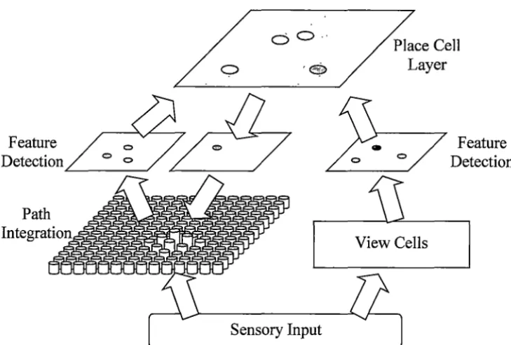
path integrator. The path integrator mimics the behaviour of the attractor model proposed by Kali and Dayan (2000). Path integration is implemented as a moving hill of activity on a two dimensional array of cells. The position of this hill represents the position of the animal, and is moved by applying movement information or information from the place cell layer. Connections between the path integration layer and the place cell system are mediated by feature detection layers as shown in Figure 3.2. Connections between these and other layers are modified using a form of competitive Hebbian learning. Each place cell responds to features present in the path integration layer and in the view layer.
Feature Detection
C) 0 - ·
~ceCell
/ .°Layer
"-~~~~~~~---J
View Cells
Sensory Input
[image:38.562.121.486.272.518.2]Feature Detection
Figure 3.2: Simplified overview of the computational model of Guazelli, Bota and
Arbib (2001 ).
summary
3. 1.4. Kalman Filtering
All of the models discussed share a similar philosophy based on observations of biological systems. The basic process is to identify landmarks in the sensory view and extract information about the relative positions of those landmarks, this information can then be combined with estimates from a path integrator for more robust localisation. An alternative approach is to examine non-biological methods for achieving the same result and then to relate these back to the biological solutions.
A Kalman filter (Jazwinski, 1970) estimates the state of a dynamic system by combining a series of noisy state observations and on a model of how the state may change. In the case of robotic localisation, the state is the location of the robot, state observations are sensor input, and state changes are indicated by motor outputs, wheel rotation or some other measure of change in position. Under certain conditions, a Kalman filter can be shown to provide optimal update rules for combining uncertain information (Bousquet, Balakrishnan, & Honavar, 1997). Figure 3.3 depicts the basic Kalman filtering concept.
Prediction
State
Predicted
Estimate
Measurement
State
Estimate
Actual
Observed
Update
State
Measurement
Observation
Figure 3.3: A schematic of Kalman filtering (adapted from Balakrishnan, Bhatt, &
Honavar, 1998).
Figure 3.4. They argue that the function of the hippocampus during localisation is the same as that of a Kalman filter.
Actual Position
Place Code
CA3
Prediction
Position Estimate
dead-reckoning
Field Centre
CAI
Observation
Position Estimate
"'>---I-___... Field Centre
Update
Figure 3.4: Hippocampal localisation and position update procedure (adapted from
Bousquet et al., 1997).
From this observation, a computational model composed of five modules was developed as shown in Figure 3.5.
Module 5
Module 4
Module 3
Module 2
Module I
Type Pos.
Goal Memory
Position Estimate
Figure 3.5: Hippocampal model of Balakrishnan and Colleagues (Balakrishnan et
The computational model was designed to be a simplified simulation of modules 1 to 4. As is common with the biologically based model discussed in section 3.1.1, Module 1 view cell activation consists of a product of Gaussians tuned to the positions of perceived landmarks, with the type of landmark acting as an additional input. Module 2 cells respond to particular combinations of Module 1 cells, with new units being added if there is no Module 2 unit that matches the Module 1 activation. As each module 2 unit is added, it becomes iissociated with the current position estimate from the path integrator. The authors then use a modified form of the Kalman filtering algorithm to update the state estimate.
Lee and Reece (1997) also use a Kalman filter for localisation, but take a different, somewhat less biologically plausible, approach. The system was developed for a mobile robot called ARNE9. ARNE is constructed on a 300mm circular base with a
two-wheel differential drive system. The robot is equipped with a single sonar sensor that is able to rotate, and is set to take readings at every 18 degrees. Sonar readings were used to build either a feature map10 or an occupancy grid of the environment, and this map was used in conjunction with a Kalman filter to allow the robot to localise within the environment. While this system was not biologically based, it was later extended by Reece and Harris (Harris & Reece, 1997; Reece &
Harris, 1996) to include some biologically inspired features.
A limitation of the original localisation system was that it was able to perform incremental localisation only. That is, given a starting position plus odometric information and sonar data, the robot was able to estimate the new location. The extensions of Reece and Harris also allow absolute localisation. That is, the ability to localise based on current sensory information only, as when the robot first enters the environment.
The extended system included an environment memory consisting of place cells. Each place cell stored a map representation in robot-centred coordinates. In each cycle, the partial map generated by the mapping system was presented to the place cells. Each place cell received a score based on the similarity of the stored map to the partial observed map. The retrieved maps of those place cells that fire strongly were then used to assist in localisation and mapping. The authors claim that this
9 ARNE is another mid-sized mobile robot. See Lee (1996) for more information.
place system is similar to Marr's (1971) auto-associative theory of hippocarnpal function, although this connection is not made clear.
3.2. Navigation
Place cell to goal cell connections are trained using 'one-shot' Hebbian learning as each goal is encountered. These goal cells form the basis for navigation, which will be discussed in section 3.2.
3.2.1. Coordinate Based Navigation
If the place cell model includes a metric path integration system, then navigation can be achieved using a simple coordinate based procedure. The robot remembers the path integrator coordinates of the goal location and compares these to the current position estimate. Vector subtraction of these coordinates gives the direction to the goal. Such a system was used by Touretzky, Wan and Redish (1994) in their simulations. Similarly, Balakrishnan, Bhatt and Honavar (1998) used this technique, however they also included a heuristic method for choosing an appropriate goal.
\ \
\ \
\ \
\ \
\
'
,--,
/
'
I \
Goal
1I
,
[image:43.562.98.478.60.269.2]'
... -'Figure 3.6: Coordinate-based navigation is unsuitable for complex environments.
The large arrow shows the computed direction to the goal location, whereas the dashed arrow shows the optimal direction of movement.
The results of such experiments with robots and rodents are taken as evidence that rodents do maintain a coordinate representation of goal locations and the current position estimate. Unfortunately however, coordinate learning is not suitable for use in environments involving large or concave obstacles, as shown in Figure 3.6. Small convex obstacle can be navigated by moving along the object while also moving closer to the goal. However for larger and, in the worst case, concave obstacles (dead-ends) this technique will fail. Environments containing such obstacles will be referred to as complex environments.
3.2.2. Potential Fields
Gaussier and colleagues (2000; 2002) implemented navigation through the use of potential fields. When a goal is reached, the robot learns to associate nearby views with the goal by backing a small distance away from the goal and training view cells. This is repeated for movement in multiple directions. To return to the goal, the robot finds the view cell that best matches the current sensory input and moves in the direction indicated by that cell. Again, this method of navigation is only useful in simple environments, and will also be limited by the size of the environment. In addition, the complicated process of learning views for each goal limits the attractiveness of this approach.
between goal cell and place cells were learned based on the direction of movement when the goal was reached, and the recency of place cell firing. While reducing the complexity of the learning procedure, this method does not solve the problem of navigating in large complex environments.
3.2.3. Reinforcement Leaming
Reinforcement learning has long been used for low-level navigation, such as collision avoidance and wall following, and for navigation to a fixed goal (Sutton &
Barto, 1998). Unfortunately, reinforcement learning algorithms perform poorly when navigating in environments with dynamic goal locations, such as watermaze tasks (Foster et al., 2000). Reinforcement learning algorithms learn the values associated with states and actions, with respect to the current goal. If the goal location is changed, the previously learned values interfere with the new task being learned. This problem will be discussed further in section 8.1.
Foster and colleagues (2000) developed a method for combining reinforcement and coordinate learning. The agent uses the actor-critic (see Section 7 .1.1 for details) paradigm to choose between movement in each of eight discrete directions (as in conventional methods), as well as the direction computed by the coordinate system (see Section 3 .2.1 ). In open environments, the critic will learn that the coordinate system may be trusted to compute an appropriate action, enabling efficient
'
navigation with dynamic goals since the coordinates are goal independent. However in complex environments, the system will revert to the traditional reinforcement learning approach with the associated poor performance when goal locations change.
Arleo and Gerstner (2000; 2001) also used reinforcement learning for navigation. In particular, Watkins' Q-leaming was used to learn a value function from a linear approximation based on place cell activity (see section 7.1 for details). In principle, a value function can be learned for each goal location, allowing navigation in both open and complex environments with dynamic goals. This technique does not make use of coordinate information, however it should be possible to combine the method with that of Foster and colleagues.
3.2.4. Hierarchical Navigation
moves. The CA3 layer learns associations between place cells with neighbouring place fields. These associations are direction specific, so that a given connection may represent a neighbour to the North, for example.
Goal cells code for where the animal is in relation to each goal, with one goal cell for each direction (eg. North, East, South and West). When the animal reaches a goal, it triggers the CA3 connections in each direction and the propagation of neighbouring cells allows connections to be learned between the appropriate goal cell and all place cells in that direction. The major limitation of this form of navigation is that, like the coordinate techniques, the model is limited to simple environments without obstacles. This issue was addressed in a later refinement (Trullier & Meyer, 1998).
The extended model includes the notion of sub-goals. When the robot is at a location where goal information is not available, it moves around until it finds a location where goal information is available. At this point, a new set of sub-goal cells is recruited for the current location. Eventually enough sub-goal cells will be recruited to enable navigation from any location within a complex environment. However, this approach does not fit experimental observations, since it requires several visits to the goal location in order to learn enough sub-goals to enable successful navigation in complex environments. In contrast, rats are able to return to the goal after only one trial in the same situation.
Reinforcement learning has also been used with a similar hierarchy of goal states (Dayan & Hinton, 1993; Dietterich, 1998; D!gney, 1996; Kaelbling, 1993a; Parr &
Russell, 1997; Singh, 1992). These techniques show great promise for robust navigation in complex environments, and for reducing the time complexity of reinforcement learning algorithms (see Section 8.2.5).
3.3.
Low-Level Navigation3.4. Summary
This chapter has reviewed some of the major biologically inspired systems for localisation, mapping and navigation. The general approach to localisation is quite consistent and involves the combination of view and odometric input to establish place units. However, the models differ in the way that this information is used, and in the way that cognitive maps are addressed. Some models maintain explicit representations of maps, whereas in other models, the maps are implicit or not present.
Chapter 4. System Design
The main objective ofthis research is to develop an autonomous navigational system for a simulated mobile robot based on biological principles. The system will provide navigational abilities in typical real world environments, and should rely on simple sensory systems only.
Real world environments are typically complex and cluttered, with many obstacles, dead ends and potential shortcuts. They are also rarely static and may involve doors, movable obstructions, people or other robots. Ideally, a navigational system will be able to deal efficiently with all of these situations, without requiring complex and expensive sensors. Simple, inexpensive sensors that are commonly used on mobile robots include sonar and infrared rangefinders, bumpers for collision detection, and various devices for measuring odometric information, such as wheel rotation. A carefully designed bumper system is generally error and noise free. However, measurements from inexpensive rangefinders (especially sonar) and odometric devices may contain considerable noise, and/or be error prone. While generally noisy, sonar readings are also subject to misinterpretation resulting from specular reflections, echoes, and weak returns. Odometric readings are often very precise, but if measuring wheel rotations, for example, may introduce errors due to wheel slip and collisions, hence the resulting accuracy is usually quite poor, especially since these errors have a cumulative effect. The navigational system will need the ability to overcome the limitations of these sensors.
Two essential components of any navigational system are localisation and navigation. That is, the ability to determine the current position and the ability to deduce appropriate actions to reach the current goal. This chapter will describe the general design of the proposed system with reference to the previous models discussed in Chapter 3.
4.1. Localisation
of metal objects or power lines. Gyroscopes and accelerometers for tracking changes in direction are considerably more accurate, but these may introduce a small drift to the perceived heading, which is extremely undesirable when this reading is used to calculate changes in position. However, a careful combination of measurement devices can lead to reasonably robust head-direction systems (e.g. Benson, Stombaugh, Noguchi, Will, & Reid, 1998; Kim & Seong, 1996). Alternatively, an attractor based head-direction network, such as those used by Skaggs and colleagues (1995), may be used to maintain head-direction. As a further alternative, the place cell system preposed below could easily be modified to also correct head-direction. Given the many options available for maintaining a robust estimate of head-direction, this thesis will tackle only the more difficult problem of maintaining a positional estimate. However, care will be taken to ensure that the system is not overly dependent on an accurate head-direction estimate, although it is assumed that any global drift will be corrected.
Figure 4.1 shows the basic structure of the proposed system.
Localisation Module:
View Cells Path Integration Place Cells
Position
Figure 4.1: Localisation module.