The effects of model structure and complexity on the behaviour and performance of marine ecosystem models

(1)

The effects of model structure and complexity on the behaviour and

performance of marine ecosystem models.

by

Elizabeth Ann Fulton; BSc Hons

Submitted in fulfilment of the requirements for the Degree of Doctor of Philosophy

(2)

Declarations

Originality

I declare that this thesis is my own work and contains no material that has been accepted in any form for another degree or diploma by the University of Tasmania or any other

institution, except by way of background information that is duly acknowledged in this

thesis. To the best of my knowledge and belief no material within this thesis has been published or written by another person except where due acknowledgment is made in

the text of the thesis.

(signature) Elizabeth Ann Fulton

Authority of Access

I declare that this thesis may be made available for loan and limited copying in accordance with the Copyright Act 1968.

Qo/1/.16-‘)

z_

(signature) (date)

Elizabeth Ann Fulton

(3)

Abstract

Despite increasing use of ecosystem models, the effects of model structure and

formulation detail on the performance of these models is largely unknown. Two

biogeochemical marine ecosystem models were constructed as the foundation of a study

considering many aspects of model simplification. The models use a trophic web that is resolved to the level of functional groups (feeding guilds), and includes the main pelagic

and benthic guilds from primary producers to high-level predators. Both models are process based, but the Integrated Generic Bay Ecosystem Model (IGBEM) is highly

physiologically detailed, while Bay Model 2 (BM2) uses simpler general assimilation equations. Both models compare well with real systems under a wide range of

eutrophication and fishing schemes. They also conform to general ecological

checkpoints and produce spatial zonation and temporal cycles characteristic of natural

systems. The performance of IGBEM is not consistently better than that of BM2,

indicating that high levels of physiological detail are not always required when

modelling system dynamics. This was reinforced by a section of the study that fitted

BM2, IGBEM and an existing ecosystem model (ECOSIM) to Port Phillip Bay. The predictions of all three models lead to the same general conclusions across a range of

fishing management strategies and scenarios for environmental change.

Models that are less resolved or use simpler formulations have lower

computational demands and can be easier to parameterise and interpret. However, simplification may produce models incapable of reproducing important system

dynamics. To address these issues simplified versions of BM2 and IGBEM were

compared to the full models to consider the effects of trophic complexity, spatial

resolution, sampling frequency and the form of the grazing and mortality terms used in

(4)

or very simplistic linear grazing and mortality terms is misleading, especially when ecosystem conditions change substantially. The research indicates that for many facets

of model structure there is a non-linear (humped) relationship between model detail and

performance, and that there are some guiding principles to consider during model

development. Developmental recommendations include using a sampling frequency of 2

—4 weeks; including enough spatial resolution to capture the major physical

characteristics of the ecosystem being modelled; using quadratic mortality terms to

close the top trophic levels explicitly represented in the modelled web; aggregating species to the level of functional groups when constructing the model's trophic web, but

if further simplification of the web is necessary then omission of the least important

groups is preferable to further aggregation of groups; giving careful consideration to the

grazing terms used, as the more complex lolling type responses may be sufficient; and if an important process or linkage is not explicitly represented in the model, or is poorly

known, then a robust empirical representation of it should be included.

The work presented here also has implications for wider ecological topics (e.g.

the stability-diversity debate) and management issues. Consideration of the effects of

trophic complexity on model performance under a range of environmental conditions

supports the ecological "insurance hypothesis", but not the existence of a simple

relationship between diversity and stability. The biological interactions captured in the web are a crucial determinant of ecosystem and model behaviour, but simple aggregate

measures such as diversity, interaction strength and connectance are not. Similarly, the

work on the effects of spatial resolution on model performance indicates that spatial heterogeneity is a crucial system characteristic that contributes to many of the emergent

properties of the system.

(5)

to eutrophication than to fishing. Second, a selected set of indicator groups can signal

and characterise the major ecosystem impacts of alternative management scenarios and

large-scale changes in environmental conditions. Third, policies focusing on the

protection of a small sub-set of groups (especially if they are concentrated at the higher

trophic levels) can fail to achieve sensible ecosystem objectives and may push systems

into states that are far from pristine. Fourth, multispecies and ecosystem models can identify potential impacts of anthropogenic activities and environmental change that a

series of single species models cannot. Finally, and most importantly, the use of a single

"ultimate" ecosystem model is ill advised, but the comparative and confirmatory use of

(6)

Acknowledgments

As with any body of work this large there are many, many, people who

contributed in some way to its completion (or at least to the survival of the author).

There are probably far too many to mention all of them by name, but there are some that

deserve special attention.

Firstly, I'd like to thank Shell Australia and the CSIRO Division of Marine

Research for providing my scholarships. I'd also like to thank the CSIRO Division of

Marine Research and the School of Zoology, University of Tasmania for funding my

research.

With regard to help, advice and inspiration in all matters technical and model

related I'd like to give special thanks to Jerry Blackford, Adam Davidson, Sandy

Murray, Francis Pantus, Jason Waring and Stephen Walker. Thank you also to Robert Bell, Andy Edwards, Lars HAkanson, Xi He, Jaques Nihoul, Keith Sainsbury, Bill

Silvert, Carl Walters and Andy Yool for their willingness to participate in discussions

about modelling and model complexity. In particular, I'd like to thank Sandy Murray

for facilitating the extension and modification of PPBIIM, and John Parslow for his very

thoughtful (and thought provoking) comments, insights and discussions during the entire course of this research — the models are all the better for them!

Moving into areas less technical, but nonetheless important, I'd like to thank the

multitude of people who supported and tolerated me during this period. Thanks to my comrades in arms (Joe, Hugh, Piers, Jeff, Alice, Dirk, Phil and Reg) for the friendship

and offers of beer over the last few years (it was all heartily appreciated even if I didn't drink the beer!). A very big thankyou to the Block 3 support crew (Nikki, Bronwyn,

Wendy and Tilla) who have been there from the start (when even I wasn't sure what I

was doing). An equally huge thank you to the Block 1 crew (David, Helen, Rich, Robin

(7)

of laughs to keep me going.

Lastly, to those people I couldn't have done without. Thanks to all my friends,

near and far, who were interested enough to ask how it was going and polite enough to sit through my answer. Thanks must go to Craig Johnson for putting up with an esoteric

student who still thinks isopocis look like underwater cockroaches. A family sized

thankyou goes to the Smiths for all their generosity, in particular to Tony who is worth immeasurably more than his weight in gold. A very big hug and thankyou to Jim whose

daily e-mails were a pleasure to look forward to — on top of which he kept a better

countdown than I ever could! And last, but never least, my family. I could not have

done it without your love and support (Mum you can stop stressing now!). In particular,

big, big hugs to the brave souls who travelled through this with me, Derek, Lachy,

Janneke and Mei (?), I love you very, very much!!

Dedication

(8)

List of Figures

Figure Number Page Number

Figure 1.1: Map of box geometry used for the standard runs of IGBEM 10

Figure 1.2: Biological and physical interactions between the components

used in IGBEM 14

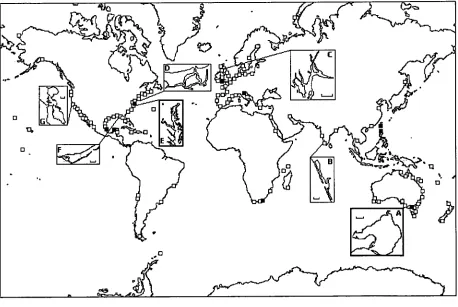
Figure 1.3: Map of the world showing the bays used to evaluate the

performance of IGBEM 24

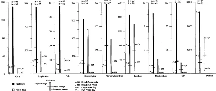
Figure 1.4: Ranges and average values for the main sets of the model

(IGBEM) in comparison with field values worldwide 27

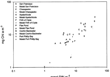
Figure 1.5: The relationship between the mean annual concentration of

DIN and chl a for real and modelled microtidal marine systems 32

Figure 1.6: The relationship between the mean annual concentration of DIN and chl a for a selection of real and model microtidal marine

systems 32

Figure 1.7: Relationship between the maximum depth and the average biomass of meiobenthos in the sediments of real and modelled

coastal marine systems 33

Figure 1.8: Growth curves for fish groups as produced by the model and

the species their parameterisations are based on 38

Figure 1.9: Maps of the location of the physical and biological areas

identified in the output of the PM run 41

Figure 1.10: Maps of the location of the physical and biological areas

identified in the output of the CM run 46

Figure 1.11: Relative biomass through time showing temporal patterns for

(14)

Figure Number Page Number Figure 2.1: Map of the geometry used for the standard runs of BM2 65

used in BM2 . 66

Figure 2.3: Map of the world showing the bays used to evaluate the

performance of BM2 . 71

Figure 2.4: Range and average value for each of the main trophic sets of BM2 compared with values from empirical observations

and from the output of IGBEM 73

Figure 2.5: Comparison of the mean annual DIN against mean annual

chl a for real microtidal marine systems, BM2 and IGBEM . 79

Figure 2.6: Plot of the average biomass of meiobenthos against maximum depth of the system for marine systems from around the globe,

BM2 and IGBEM 79

Figure 2.7: Maps of the biological and physical areas identified by the MDS, cluster and correlation analysis of the runs using the

loadings for Port Phillip Bay (the PM run) of BM2 and IGBEM 81

Figure 2.8: Maps of the biological and physical areas identified by the MDS, cluster and correlation analysis of the runs using the

loadings for Chesapeake Bay (the CM run) of BM2 and IGBEM 82

Figure 2.9: Distribution of the main zones identified in the output of

BM2 and IGBEM 83

Figure 2.10: The biomass through time for the aerobic bacteria in box 23

(15)

Figure Number Page Number Figure 2.11: Declines in biomass of the demersal and planktivorous fish

with an increase in fishing for the standard run of BM2 and the run

using Beverton-Holt recruitment 93

Figure 3.1: The specific bays chosen to set alternative nutrient load

scenarios for BM2 . 102

Figure 3.2: Average value for the zooplankton in BM2, in comparison

with values for those sets in the field and in the output of IGBEM 106

Figure 3.3: Spatial distribution of the main communities identified in the PM run of BM2 and IGBEM, as well as those recorded

in PPB . 113

Figure 3.4: Distribution of the main communities distinguished in

the CM run of BM2 and IGBEM 115

Figure 4.1: Trophic webs of BM2 and IGBEM 127

Figure 4.2: Maps of the geometries used with the models . 129

Figure 4.3: Variance of chlorophyll a in the "Yarra River" box over the final 4 years of the 20 year runs for different levels of

spatial resolution in the BM2 and IGBEM models . 131

Figure 4.4: Variance in the bay-wide average chlorophyll a over the final 4 years of the 20 year run for different levels of spatial

resolution in the BM2 and IGBEM models . 132

Figure 4.5: Effects of spatial resolution on self-simplification 135

Figure 4.6: Effects of spatial resolution on the spatial distribution of

functional groups . 138

Figure 4.7: Time-series of denitrification as defined by each of the

(16)

Page Number Figure Number

Figure 4.8: Ratio of the estimated and true values of pelagic (water column) and benthic primary production for BM2 and IGBEM under various sampling frequencies .

Figure 4.9: Ratio of the estimated and true values of production by benthic filter feeders BM2 and IGBEM under various sampling

frequencies

Figure 4.10: Ratio of the estimated and true values of pelagic primary production for IGBEM under various sampling frequencies with

baseline nutrient conditions and a fivefold increase in nutrient

load .

Figure 4.11: Ratio of the estimated and true values of pelagic secondary production for IGBEM under various sampling frequencies with

baseline fishing conditions and a fivefold decrease in fishing

pressure

Figure 5.1: Diagrams of the most common system configurations that are simplified by aggregating groups.

Figure 5.2: Food web diagram for the ecosystem models BM2 and IGBEM .

Figure 5.3: Plot of connectance (C) and the number of links in the simplified food webs produced by aggregating components,

against the number of groups in the webs

Figure 5.4: Plot of connectance (C) and the number of links in the simplified food webs, produced by omitting components,

against the number of functional groups in the webs.

146

147

149

160

163

174

(17)

Figure Number Page Number Figure 5.5: Plots of the absolute relative differences in the predicted

values of indices between the simplified (with aggregated

trophic groups) and full versions of the models in relation

to the number of groups included in the models 177

Figure 5.6: Relative differences between the chlorophyll a concentrations provided by the simplified (with aggregated trophic groups)

and full models 180

Figure 5.7: Comparison of the temporal dynamics of "large zooplankton" in LP2, the time series produced by adding the time series for "small zooplankton" and "large zooplankton" in LA6 and the time series

produced by adding the time series for all the zooplankton groups

in the standard (full) version of Bay Model 2 (BM2). 182

Figure 5.8: Comparison of the temporal dynamics of chl a in one cell of the standard model and versions of BM2 with aggregated

groups. 182

Figure 5.9: Plot of the absolute relative differences in the predicted values of indices between the simplified (with omitted trophic groups) and full versions of the models in relation to the

number of groups included in the models 184

Figure 5.10: Absolute relative differences between estimates of primary production between models with omitted groups and the full

model . 186

Figure 5.11: Absolute relative differences between estimates of consumption between models with omitted groups and the full

(18)

Figure Number Page Number Figure 5.12: Comparison of the temporal dynamics of epifaunal

predators in one cell of the full IGBEM model and versions

with omitted groups . 190

Figure 5.13: Comparison of the temporal dynamics of the biomass of diatoms in one cell of the full BM2 model and versions

with omitted groups . 190

Figure 5.14: Comparison of the temporal dynamics of the biomass of diatoms in one cell of the full BM2 model and versions with omitted groups when nutrient loads have been increased by

fivefold 195

Figure 5.15: Plot of the ratio of interaction strength (strong:weak) for the

BM2 runs simplified by omitting groups . 201

used in BM2 . 209

Figure 6.2: Spatial structure implemented for BM2 . 210

Figure 6.3: Proportion of the total average biomass of heterotrophic flagellates in each box for each run with alternative grazing

formulations . 219

Figure 6.4: An example of only minor differences in time-series for

alternative forms of model closure 231

Figure 6.5: An example of major differences in time-series for alternative

forms of model closure 231

Figure 6.6: The "type 1", "type II" and "type HI" functional responses

(19)

Figure Number Page Number Figure 7.1: Schematic diagram showing the groups in BM2 and IGBEM

and their relative trophic positions 252

Figure 7.2: Depth map of Port Phillip Bay, Melbourne, Australia . 253

Figure 7.3: Schematic diagram of the Port Phillip Bay ECOPATH model,

showing the constituent groups and their relative trophic positions . 259

Figure 7.4: Overlay of a section of the time series of the Benthic Deposit

Feeder group in all three models 273

Figure 7.5: Overlay of a section of the time series of total phytoplankton

for the three models . 273

Figure 7.6: Overlay of a section of the time series of the planktivorous

fish group (clupeoids) in all three models 274

Figure 7.7: Plot of ECOSEVI biomass trajectories under the Fs that result

from an economically oriented objective function . 282

Figure 7.8: Plot of ECOSIM biomass trajectories under the Fs which

result from an ecologically oriented objective function 283

Figure 7.9: Plot of ECOSIM biomass trajectories under the Fs which result from an objective function that is weighted for a

compromise of the ecological and economic strategies 287

Figure 7.10: Plot of ECOSIM biomass trajectories under the split Fs which result from an economically oriented objective function

applied when there is a drop in productivity . 295

Figure 8.1: Plot of articulation against effectiveness for a number of

existing aquatic models 324

Figure 8.2: Plot of predictive power / accumulated error against the

(20)

List of Tables

Table Number Page Number

Table 1.1: List of components in IGBEM compared to those in PPBIM

and the biological modules of ERSEM H 13

Table 1.2: Level of detail used in the model formulation for each of

the processes carried out in a standard run of IGBEM 15

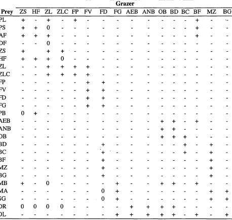
Table 1.3: Diet matrix for the living components in a standard run

of IGBEM . 17

Table 1.4: Alternative regimes for fish recruitment implemented

in IGBEM 22

Table 1.5: Comparison of the community composition for the benthic and fish communities determined from empirical estimates in

PPB and the PM model run . 29

Table 1.6: Summary of the Sheldon spectra for the pelagic classes in the run where nutrient loads were at the levels recorded in Port

Phillip Bay (PM run) and Chesapeake Bay (CM run) 34

Table 1.7: Summary of the Sheldon spectra for the benthic classes in the

baseline (PM) and nutrient load x10 (CM) runs of IGBEM . 35

Table 1.8: Estimates of primary and secondary production and

consumption for PPB and the PM run of IGBEM . 36

Table 1.9: System level indices for a range of real coastal areas and three

separate runs of IGBEM 39

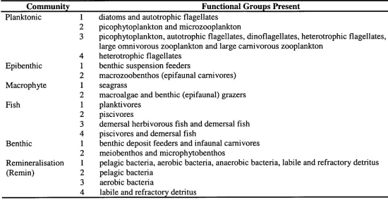
Table 1.10: Definitions for the various communities found in the output

of IGBEM runs 42

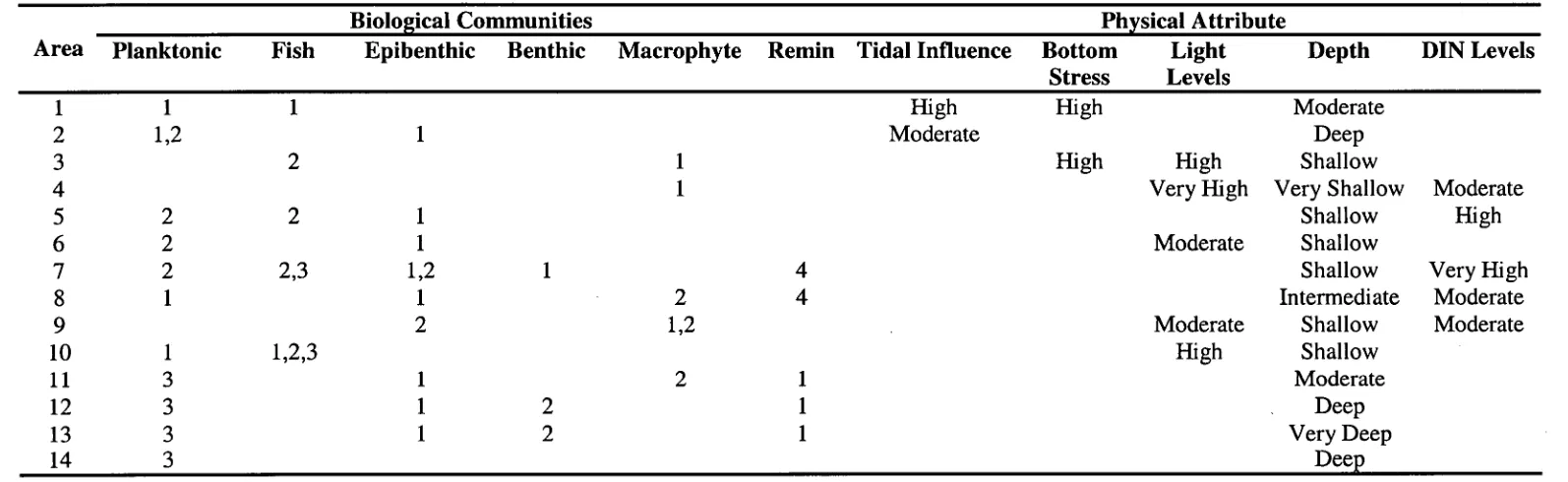
Table 1.11: Dominant communities and physical attributes characterising

(21)

Table Number Page Number Table 1.12: Dominant communities and physical attributes characterising

each biological area identified in the CM run 45

Table 2.1: Comparison of the underlying assumptions and formulations

of the standard implementations of BM2 and IGBEM 63

Table 2.2: The recruitment relationships available in BM2 . 71

Table 2.3: A summary of the Sheldon spectra for the pelagic classes in the run of BM2 and IGBEM where the environmental conditions

match those in Port Phillip Bay 77

Table 2.4: A summary of the pooled Sheldon spectra for the benthic classes in the run of BM2 and IGBEM where the environmental

conditions match those in Port Phillip Bay . 78

Table 2.5: Relative abundance of the large and small size fractions of the phytoplankton and zooplankton communities in the runs of BM2 and IGBEM using the nutrient loadings of Port Phillip

Bay (PM run) and Chesapeake Bay (CM run) 88

Table 2.6: Steepness values for the Beverton Holt stock recruit curves

implemented for the fish groups 92

Table 3.1: Average value for each set observed in PPB and Chesapeake Bay (CB) and predicted by the associated runs (PM and CM

respectively) of BM2 and IGBEM . 104

Table 3.2: Comparison of the community composition for the fish and benthic groups observed in PPB and predicted by BM2

(22)

Table Number Page Number Table 3.3: Comparison of the estimates of the ratios of

production:biomass and consumption:biomass for PPB and the

BM2 and IGBEM runs with conditions matching those in PPB 109

Table 3.4: List of indices and their associated values for PPB and the runs of the ecosystem models BM2 and IGBEM where

the environmental conditions reflect those found in PPB

(the PM run) or Chesapeake Bay (the CM run) 111

Table 3.5: Dominant groups distinguishing the "edge" and

"central" communities 114

Table 3.6: Meaning of the codes used in Table 3.5 . 115

Table 4.1: Comparison of the underlying assumptions and formulations

of the standard implementations of BM2 and IGBEM 126

Table 4.2: Persistence of the trophic groups in runs of BM2 and IGBEM

using 8-box, 3-box and 1-box geometries 133

Table 4.3: Relative biomass, production and consumption for the runs

of BM2 and IGBEM on the smaller geometries 137

Table 4.4: Spatial distribution of assemblages predicted using BM2 on

59-, 8- and 3-box geometries . 139

Table 4.5: Groups demonstrating different responses to spatial structure

under alternative amounts of fishing and nutrient loads in BM2 141

Table 4.6: Groups demonstrating different responses to spatial structure

under alternative amounts of fishing and nutrient loads in IGBEM . 142

Table 4.7: Summary of the impact of changes in nutrient loading or

fishing pressure on the effects of sampling frequency 147

(23)

Table Number Page Number Table 5.1: List of the biological components in the full versions of

BM2 and IGBEM . 164

Table 5.2: Processes and structure of BM2 and IGBEM . 165

Table 5.3: List of the trophic simplifications of the food web made

by aggregating groups. 167

Table 5.4: List of the trophic simplifications of the food web made by

omitting groups. 169

Table 5.5: List of the trophic simplifications (models) considered

under a fivefold increase in nutrient load or fishing pressure. 170

Table 5.6: Comparison of the magnitude of average relative deviation from the full models of the indices from runs produced by

aggregation and omission of groups for BM2 and IGBEM 178

Table 5.7: Overall performance indicators (V) for the simplified versions of BM2 and IGBEM, when simplification was

by aggregating trophic groups 179

Table 5.8: Categories of the effects of aggregating groups on the relative spatial distribution of the constituent components,

and associated processes, in BM2 and IGBEM 180

Table 5.9: Overall performance indicators (V) for runs of BM2 and

IGBEM, with groups omitted from the models 188

Table 5.10: Categories of the effects of omitting groups on the relative spatial distribution of the constituent components, and associated

(24)

Page Number Table Number

Table 5.11: The effects of model simplification by aggregation on the relative spatial distribution of the constituent components, and associated processes, in BM2 and IGBEM when the nutrient

load or fishing pressure is increased to five times that of the

"baseline" conditions.

Table 5.12: The effects of omitting groups on the relative spatial distribution of the constituent components, and associated processes, in BM2 and IGBEM when the nutrient load or fishing

pressure is increased to five times that of the "baseline"

conditions

Table 5.13: Predicted change in biomass of macrophytes for standard (full) model and versions of BM2 with aggregated groups

Table 6.1: Biologically associated components present in BM2

Table 6.2: Alternative formulations of the grazing term per consumer considered .

Table 6.3: List of the identifying names given to the runs and sets of forcing conditions discussed in this paper .

Table 6.4: Proportional difference between the biomass predicted in the "standard" run and those runs using alternative grazing

formulations .

Table 6.5: Number of boxes for which the relative spatial distributions of the "standard" run differs from that predicted by the runs

using an alternative grazing term

192

193

193 208

212

215

218

(25)

Page Number Table Number

Table 6.6: Quality of the match between the predicted time-series for each component in the "standard" run and those runs using

alternative grazing formulations

Table 6.7: Proportional difference in the size of the trends predicted in the "standard" run and those runs using alternative grazing

formulations when the nutrient load is increased fivefold .

Table 6.8: Proportional difference in the size of the trends predicted in the "standard" run and those runs using alternative grazing

formulations when the fishing pressure is increased fivefold

Table 6.9: Number of boxes for which the relative spatial distributions of the "standard" run differs from that predicted by the runs

using an alternative grazing term when forcing conditions are

changing

Table 6.10: Quality of the match between the predicted time-series under changing forcing conditions for each component in the

"standard" run and those runs using alternative grazing

formulations .

Table 6.11: Proportional difference between the biomass predicted in the "standard" run and those runs using alternative forms of

model closure .

Table 6.12: Number of boxes for which the relative spatial distribution of the "standard" run differs from that predicted by the runs using an alternative forms of model closure .

221

222

223

225

226

227

(26)

Table Number Page Number Table 6.13: Quality of the match between the predicted time-series for

each component in the "standard" run and those runs using

alternative forms of model closure 230

Table 6.14: Proportional difference in the size of the trends predicted in the "standard" run and those runs using alternative forms of

model closure when the fishing pressure is increased fivefold 232

Table 6.15: Proportional difference in the size of the trends predicted in the "standard" run and those runs using alternative forms of model

closure when the nutrient load is increased fivefold . 233

Table 6.16: Number of boxes for which the relative spatial distributions of the "standard" run differs from that predicted by the runs using

an alternative forms of model closure when forcing conditions

are changing . 235

Table 6.17: Quality of the match between the predicted time-series under changing forcing conditions for each component in the

"standard" run and those runs using alternative forms of model

closure. 236

Table 7.1: Comparison of the underlying structure and assumptions of

the three ecosystem models, ECOSIM, IGBEM and BM2 248

Table 7.2: Process detail involved in the phytoplankton production for

each model . 250

Table 7.3: The basic input parameters for the Port Phillip Bay ECOPATH

model . 255

Table 7.4: Landings, discard and total value information for the harvest

(27)

Table Number Page Number Table 7.5: Criteria used to define the objective functions used in the

ECOSIM policy analysis routines 266

Table 7.6: Comparison of the group data for the three models 268

Table 7.7: A comparison of ten system level indices for the "base case"

runs of the three models 271

Table 7.8: The relative change in biomasses for each of the three models

under the test scenarios 276

Table 7.9: System level indices for all the simulations 278

Table 7.10: Results of the policy analyses under constant environmental

conditions 280

Table 7.11: Comparison of the important "economic", "ecological" and

"intermediate" strategies 288

Table 7.12: The relative change in biomasses for each of the three models

under the ecological and economically based strategies 289

Table 7.13: Results of the policy analyses under changing environmental

conditions 293

Table 7.14: Changes in biomass that result from the implementation of

the suggested optimal fisheries policies 299

Table 7.15: Summary of the major conclusions and supporting results

from the three ecosystem models considered here 303

Table 8.1: Summary of the main strengths and weaknesses associated

with the main types of multispecies and ecosystem models . 315

Table A.1: DIN, chi a and primary production for real bays. 392

Table A.2: Zooplankton biomass, production and consumption for

(28)

Table Number Page Number Table A.3: Fish biomass, production and consumption for real bays 395

Table A.4: Biomass of benthos and meiobenthos, maximum water

depth, and total benthic production and consumption for real bays 399

Table A.5: Macrophyte biomass and primary production for real bays 403

Table A.6: Total detritus for real bays 404

Table A.7: Biomass and primary production of tnicrophytobenthos

for real bays . 404

Table B.1: List of the acronyms commonly used in this thesis 406

Table B.2: List of components in BM2 and IGBEM, compared to those

in PPBIM 406

Table B.3: List of main terms used in the equations in the appendices

(29)

General Introduction

The question in context

Over the last few decades, and particularly within the last five years, there has

been a shift in focus in managing natural resources. For aquatic systems, attention is increasingly moving from specific system components, such as water quality or status

of fish stocks, to consideration of entire systems. Unfortunately, many of the tools to

facilitate this new focus are still in the early stages of development and understanding. A prime example is ecosystem models. These t'whole of system" models first began to

appear during the International Biological Program (liBP) in the early 1970s. However,

they soon developed a poor reputation (Jorgensen et al. 1992), as many were found not to be cost efficient (Watt 1975) and, more importantly, introducing detail to reflect a

growing knowledge base did not necessarily produce good model performance (O'Neill

1975, Silvert 1981, DeCoursey 1992).

With the new focus on system management and substantial increases in

computing power, ecosystem models have once again found favour. Unfortunately, the

potential pitfalls encountered during the B3P remain. Greater computing power may lift

computational constraints, but it cannot solve the issues of uncertainty about model specification and the effects of model structure and detail on model performance

(Silvert 1981, Jorgensen 1994). There have been few attempts to systematically

consider the effects of model structure on model behaviour and performance,

particularly within the realm of marine models. The work presented here attempts to

give some insight into the effect of the level of detail in an ecosystem model on the

behaviour and performance of the model.

General methodology

(30)

make it difficult to evaluate the effect of model structure on performance if models with modified structure are compared using real data. However, knowledge of the effect of

model detail on performance is fundamental to informed model development,

interpretation and use. Before a robust understanding of the relationship between model

complexity and performance is attained, both data-based and formulation-based issues

must be addressed. In approaching these issues, it will be necessary to clearly separate

their individual effects.

The research discussed here considers only the effect of model formulation on

behaviour and does not attempt to consider effects of data uncertainty. A powerful

approach to ascertain the effect of model structure on model behaviour is to use a "deep

model-shallow model" comparison. In this approach a simulation model incorporating complex processes, thought to occur in nature, acts as an artificial world or "baseline" against which the performance of other (simpler) models are compared. The simulation

model is referred to as a "deep model" and the simpler models that are compared with it are referred to as "shallow models". One of the greatest advantages of this approach is

that it allows the modeller to begin with a detailed, but validated, model and then

systematically simplify it to determine the level of detail that is sufficient and

parsimonious. In addition, it separates those parts of the optimal model complexity issue

that are linked to model structure from those dependent only on data, as it deals with

perfect knowledge.

The "deep model-shallow model" comparison approach was first used to good effect by Ludwig and Walters (1981, 1985) in fisheries science. The overall approach,

of comparing simpler "assessment" models against more complex ones, has since

become a useful means of evaluating fishery harvest strategies, including stock

(31)

and Punt, 1999) or "management strategy evaluation" (Smith et al. 1999). More recently it has been extended to cover evaluations containing multi-species interactions

(Sainsbury et al. 2000, Punt et al. in press).

Biogeochemical ecosystem models were chosen as the basis for this study because they capture processes known to be physically and biologically important

determinants of ecosystem behaviour. They also represent some of the most complex

ecosystem models available and so there is a lot of scope for simplification and

consideration of the effects of many aspects of model structure on performance. Biogeochemical ecosystem models explicitly include complex trophic webs, nutrient

dynamics and recycling, temporal variation and forcing. They can also be spatially

resolved and include highly detailed process formulations. The degree of detail employed in the formulation of any one of these features may have an impact upon

model behaviour and performance. Moreover, nutrient loading and fishing are two of

the biggest anthropogenic forces on coastal marine systems, and as biogeochemical ecosystem models explicitly employ nutrients and a trophic structure spanning primary

producers to fish, it was possible to consider the robustness of any results to the effects

of changing anthropogenic forcing of the system. There are other successful types of ecosystem model that use alternative assumptions and formulations. For example,

ECOS1M (Walters et al. 1997) is a dynamic simulation model that assumes mass

balance and explicitly incorporates top-down vs. bottom-up control, but it does not

include nutrient dynamics (using biomasses only), is not explicitly spatially structured

(assumes homogeneous spatial behaviour) and does not usually incorporate temporal

forcing. While knowledge of the sensitivity of ECOSIM to facets of its structure such as the trophic complexity is necessary (Walters pers. corn.), in comparison with

biogeochemical models, ECOSIIVI and other types of ecosystem model do not readily

(32)

However, comparison of biogeochemical ecosystem models with these other types of ecosystem model is a good way of checking for the effects of underlying system and

model assumptions on model behaviour.

This thesis

The first chapter introduces the "deep" ecosystem model, referred to as the Integrated Generic Bay Ecosystem Model (IGBEM). This model is the most detailed

model used in the study and is one of two principle "deep" models in the "deep-shallow

model" comparison. Its formulation and development is presented, as is an analysis of

its performance assessed against real marine systems from around the world. This analysis indicates that the model reproduces realistic dynamics and levels of biomass

and therefore provides a sound basis for the study of model complexity and structure. In chapter 2 I introduce the second total ecosystem model developed in the

study, Bay Model 2 (BM2). This model has a two-fold purpose. First, because it is

simpler in formulation than IGBEM, it provides a form of "shallow" model. Second, it

is sufficiently detailed to also act as a "deep model" when considering the effects of model structure on behaviour by reducing detail or scope. The development and

validation of the model as a generic system is presented, and the effect of reducing

physiological detail on model behaviour relative to IGBEM is examined. The question

of whether BM2 performs as well as IGBEM is crucial because although

physiologically intensive ecosystem models are used (Baretta et al. 1995,

Baretta-Beicker and Baretta 1997) they are controversial because they have large data and

maintenance requirements (Murray and Parslow 1999b). If simpler formulations

perform as well as physiologically intensive ones then this will temper some of the

controversy surrounding complex ecosystem models.

(33)

marine bays in general, in chapter 3 I extend the analysis presented in chapter 2 to consider two specific bays (Port Phillip Bay in Australia and Chesapeake Bay in the

USA). This analysis of the effect of process detail on model behaviour considers the models' abilities in specific circumstances. Generic models are good for developing

theory and general understanding, but models are usually applied to specific locations

and there can be system specific concerns about model behaviour. Thus, consideration

of the effects of model complexity on performance in specific systems is necessary.

The fourth chapter is concerned with specific aspects of the implementation of IGBEM and BM2, and treats both models as "deep models". I address the effect of

spatial resolution and sampling frequency (the temporal spacing of output) on model behaviour and how accurately it is interpreted. These are important issues that have

been central concerns in ecology and ecological modelling for over 40 years (Huffaker

1958, MacArthur and Wilson 1967, Levins 1970, Levin 1992, Keitt 1997, Rantajarvi et al. 1998). The sampling scale (spatial and temporal) used in field studies and in models

has logistical implications (the more intensive the sampling the more it costs to collect,

store and analyse). It can also potentially affect the processes observed in the field and

how they are interpreted (Roughgarden et al. 1988, Rantajarvi et al. 1998), and in models it can impact on both model predictions (Murray 2001) and the stability of the

modelled system (Gurney and Nisbet 1978, Hassell et al. 1994, Sharov 1996, Keitt

1997).

The fifth chapter examines the effect of trophic complexity on the performance

of IGBEM and BM2. It addresses how much of the web is needed to capture the important dynamics, and the sensitivity of model performance to the way in which the

web is constructed. This is another issue that has occupied ecology and ecological modelling for decades. In ecology, the debate over the relationship between stability and

(34)

why (Odum 1953, MacArthur 1955, May 1973, Pimm and Lawton 1978, Yodzis 1981, Harding 1999, Yachi and Loreau, 1999, McCann 2000). However, as construction of

simpler models is often a goal (Iwasa et al. 1987, Sugihara et al. 1984, Lee and

Fishwick 1998), simplifying trophic complexity in models has received some attention

(Zeigler 1976, O'Neill and Rust 1979, Cale et al. 1983, Iwasa et al. 1987, Yodzis 2000). There are two main ways in which trophic webs can be simplified, either by omitting

trophic groups or by aggregating several similar groups into a single component. Both

of these methods are commonly used in developing ecosystem models, but in the past the effects of these decisions on model performance have not received equal attention as

researchers have largely concentrated on the effects of aggregating groups. Therefore,

here I consider their relative affects on model performance.

Chapter six considers two other specific aspects of model structure and its

impact on the dynamics of the BM2 model. I evaluate the form of the grazing term (or

functional response) used in the model and the way in which the model is 'closed' (the

form of the mortality terms imposed on the highest groups in the modelled web). Both aspects are recognised as potentially having considerable effects on the dynamics of

multispecies models (May 1976, Hassell and Commins 1978, Begon and Mortimer 1986, Steele and Henderson 1992, Edwards and Mindley 1999, Murray and Parslow

1999a, Tett and Wilson 2000, Gao et al. 2000), but their effect on ecosystem models has received little attention.

In chapter 7 I compare biogeochemical models, IGBEM and BM2, with another

ecosystem model, ECOPATH with ECOSIM. In this case all the models are calibrated

to Port Phillip Bay. The objectives of this part of the study are to compare the

predictions of the models under changing conditions (nutrient loads and fishing rates) or

alternative management policies, and to ascertain whether there are commonalities and

(35)

also served to examine the effect of structure on model behaviour, as the three models

are dissimilar in their data requirements, underlying assumptions, trophic complexity

and process detail. A comparative and confirmatory approach to the consideration of the potential effects of management policies and changes in ecosystem conditions, such as

the one in this chapter, is one of the most effective ways of using ecosystem models

(Reichert and Omlin 1997, Steele 1998, Duplisea 2000, Yodzis 2001a and b).

The final chapter reviews the topic of model structure and performance by synthesising the findings of the present study in the context of published work on the

(36)

Chapter 1 An Integrated Generic Model of Marine Bay Ecosystems

Abstract

The Integrated Generic Bay Ecosystem Model (IGBEM) is presented. It is a

coupled physical transport-biogeochetnical process model constructed as a basis to

explore the effects of model structure and complexity. The foundations for the model

are two existing models, the European Regional Seas Ecosystem Model II (ERSEM and the Port Phillip Bay Integrated Model (PPBIM). Additional components (such as

benthic herbivorous invertebrates) and certain sub-models (to do with sediment

chemistry and mixing) had to be incorporated or modified to allow for extra factors of

interest and a seamless amalgam of ERSEM II and PPBIM. The standard form of the entire model compares well with real systems, with similar physical features and of varying eutrophication schemes, from Chesapeake Bay through to Port Phillip Bay

Australia. Furthermore, IGBEM conforms to general ecological checkpoints and

produces spatial zonation and long term cycles characteristic of natural systems. Despite

the model taking a generalised biomass per functional group form it captures crucial system resource dynamics well and allows for some exploration of the effects of

ecological driving forces such as predation and competition.

Keywords

biogeochemical, model, ecosystem, ERSEM, Port Phillip Bay

1.1 Introduction: marine ecosystem models

There has been a proliferation of marine ecosystem models within the last two decades with literally hundreds, of varying scope and quality, in existence. Most are

(37)

couple physics and biology tend to do so by linking sub-models that approach the

respective processes in quite different ways. Physical attributes are often dealt with via a

number of common and well defined methods, including box models, specified (often Lagrangian) flows, prognostic dynamical flow models or general circulation models.

The most common methodologies employed in the biological side of ecosystem models are pooled models (which conserve some biogeochemical currency within a chain, or

small network, of compartments that represent functional groups or trophic levels),

multispecies formulations (allowing for more realistic webs) and structured population models. Generally speaking, it emerges that box models and specified flows are the best

way of considering biological processes in realistic flow environments, free of the

complexity of directly calculating the flow itself. It is also apparent that pool models

provide a useful framework for constructing a variety of models (Olson and Hood

1994). Models such as the European Regional Seas Ecosystem Model (ERSEM)

(Baretta et al. 1995) mix and match biological formulations based on trophic identity to

capture the critical performance of the different components.

The felicitous history of reductionist physical models was probably one of the driving forces behind the bloom of highly detailed deterministic ecosystem models

during the 1970s (Young et al. 1996). However, it became apparent that complicated models did not necessarily capture system dynamics well and there was a wide spread

and rapid return to simpler or more circumscribed models. With the advent of more

powerful computers and the push for an ecosystem perspective for resource and

environmental management, detailed ecosystem models are again finding some measure

of favour. While there is still debate about their usefulness for management, given their dependence on exceedingly large numbers of, often uncertain, parameter values, they

are useful for locating gaps in our current understanding as well as learning about

(38)

Bay Ecosystem Model (IGBEM) was constructed. Consequently, it is not intended as a simulated replica of any one system. For convenience it does utilise the physics of a

particular Australian bay (Port Phillip Bay, Melbourne (Figure 1.1)), but it has the

general biology and functional groups typical of most temperate bays.

IGBEM was constructed as a first step in understanding the effects of model

structure and complexity on model behaviour and thereby deriving some guidelines to optimal model complexity. Though not a strict requirement, it was thought that such an

exercise would benefit from being built upon a reference model that resembled reality

as much as possible. Here we outline construction of the model and explore its capacity

to reflect real world behaviours.

Yarra River'

Elwood Canal'

Mordialloc Creek'

Patterson Creek+

Werdbee River* Werribee

Treatment Plant'

et

,74

t

Corlo Bar

Kororoit Creek+

Depth (m)

°

25

so Swan B

Bass Strait Boundary Condition Box

[image:38.558.113.443.371.630.2]

Great Sands*

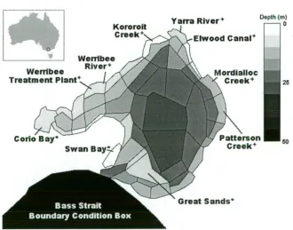
Figure 1.1: Map of box geometry used for the standard runs of the Integrated Generic

Bay Ecosystem Model. It represents Port Phillip Bay, Melbourne, Australia (location

(39)

1.2 Building IGBEM

Port Phillip Bay (PPB) has a number of features that make it an attractive site for learning. It is a large marine embayment, approximately 1930 lcm2, that has over half its

volume in waters less than 8 m (it is 24m at its deepest point). Only 8 drainage basins directly run off into the bay. Extensive sandbars form a tide delta in the southern end of

the bay and these restrict exchange between the bay and the open waters of Bass Strait.

This physically contained environment is therefore free of many of the often-worrisome

issues that are associated with boundary conditions. Since approximately three million people reside within the urbanised portions of the bay's catchment area, the bay is also

under some of the stresses faced by other major temperate bays. Accordingly it is a

prime site to study ecosystem dynamics, human impacts and how they might best be

modelled. Fortuitously it has also been the subject of intensive study over many years, which provides an extensive knowledge base to build from.

The biogeochemical model created as part of the most recent PPB study is both

detailed and successful (Murray and Parslow 1999a). However, as it is based on the

biogeochemistry of only the lower trophic levels it is not a suitable vehicle for the

examination of the effects of ecosystem model complexity and formulation, when

considering fisheries and eutrophication simultaneously. Since the Port Phillip Bay Integrated Model (PPBIM) by Murray and Parslow (1999a) does not cover enough•

faunal groups, it was necessary to use another model to extend PPBLM to produce a

suitable generic model. The European Regional Seas Ecosystem Model II (ERSEM

(Baretta et al. 1995, Baretta-Bekker and Baretta 1997) is well suited to being grafted to

PPBIM, as it is a marine biogeochemical boxmodel with a similar architecture and it includes more process detail than PPBIM and additional faunal groups. Between them,

PPBIM and ERSEM II include most of the major groups and processes thought to be

(40)

models.

IGBEM was created by tying together the biological and physical sub-models of

PPBEVI (Murray and Parslow 1997 and 1999a) and the biological modules from

ERSEM II (Baretta et al. 1995, Baretta-Bekker and Baretta 1997). The 4 submodels of

PPBIM, 3 biological ones (water column, epibenthic, sediment) and a physical

submodel, formed the framework for IGBEM and the various ERSEM II modules were

translated and added directly to the appropriate sub-model. For those functional groups

that are covered by both ERSEM II and PPBLM both formulations are included in

IGBEM with a switch setting determining which is in use in any one run. Only the ERSEM II formulations were employed in the runs presented here.

The final form of IGBEM provides a spatially and temporally resolved model of

nutrient cycles in an enclosed temperate bay. The model has twenty-four living

components, two dead, five nutrient, six physical and two gaseous components (Table

1.1). These components are linked through both biological and physical interactions and

the resultant network (Figure 1.2) is reminiscent of flow diagrams for real systems. The model is replicated spatially using the 3 layer (water column, epibenthic, sediment), 59-

box geometry developed for PPBIM. Thus, the set of polygons and their bathymetry

map a physical area that represents PPB (Figure 1.1). Temporally, a daily time-step is

utilised for the standard runs of IGBEM as this best matches the transport model which underlies the physical sub-model of IGBEM, and is little different from that of PPBIM.

The use of the transport model means that, like PPBIM, IGBEM is driven by seasonal

variations in solar irradiance and temperature, as well as nutrient inputs from point

sources, atmospheric deposition of dissolved inorganic nitrogen (DIN) and exchanges with the Bass Strait boundary box. Further details of the transport model, the rationale

(41)

IGBEM formulations and IGBEM's diet matrix are outlined in Tables 1.2 and 1.3

[image:41.559.82.503.218.749.2]

respectively.

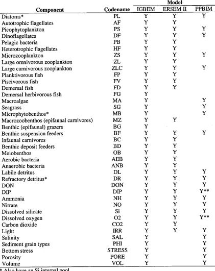
Table 1.1: List of components in the Integrated Generic Bay Ecosystem Model

(IGBEM) compared to those in the Port Phillip Bay Integrated Model (PPBIM) and the biological modules of the European Regional Seas Ecosystem Model II (ERSEM II). All living and dead components have C, N and P pools.

Component Codename

Model

IGBEM ERSEM II PPBIM

Diatoms* PL Y Y Y

Autotrophic flagellates AF Y Y

Picophytoplankton PS Y Y Y

Dinoflagellates DF Y Y Y

Pelagic bacteria PB Y Y

Heterotrophic flagellates HF Y Y

Microzooplankton ZS Y Y Y

Large omnivorous zooplankton ZL Y Y

Large carnivorous zooplankton ZLC Y Y Y

Planktivorous fish FP Y Y

Piscivorous fish FV Y Y

Demersal fish FD Y Y

Demersal herbivorous fish FG Y

Macroalgae MA Y Y

Seagrass SG Y Y

Microphytobenthos* MB Y Y

Macrozoobenthos (epifaunal carnivores) MZ Y Y

Benthic (epifaunal) grazers BG Y

Benthic suspension feeders BF Y Y Y

Infaunal carnivores BC Y Y

Benthic deposit feeders BD Y Y

Meiobenthos OB Y Y

Aerobic bacteria AEB Y Y

Anaerobic bacteria ANB Y Y

Labile detritus DL Y Y Y

Refractory detritus* DR Y Y Y

DON DON Y Y Y

DIP DIP Y Y y**

Ammonia NH Y Y Y

Nitrate NO Y Y Y

Dissolved silicate Si Y Y Y

Dissolved oxygen 02 Y Y y**

Carbon dioxide CO2 Y Y

Light IRR Y Y Y

Salinity SAL Y Y

Sediment grain types PHI Y Y

Bottom stress STRESS Y Y

Porosity PORE Y Y

Volume VOL Y Y

* Also have an Si internal pool.

(42)

Mesozoonlangon ZL Omnivorous ZLC Carnivorous

411 Organ'c matter DL Labile DR Refractory Phytoplankton Diatoms Autotrophic Flagellates Dinoflagellates Picophytoplankton Microphytobenthos* Benthic Gases 02 Oxygen CO2 Carbon Dioxide PL AF DF PS MB Zoobenthos Benthic Grazers Deposit Feeders Suspension Feeders

Meiobenthos ₄₁₄ Epibenthic Carnivores Carnivorous Infauna

Key

Living State Variable Group

Dead/Gas/Nutrient State Variable Group Other Variables/ Constant Loss Terms Flow of Matter Flow of a Nutrient Flow of a Gas Intra-group processes

L _ _

Organic Matter Labile Refractory Sediment Bacteria AEB Aerobic Bacteria ANB Anaerobic Bacteria

BG BD

—11"-13 F

OB MZ BC •

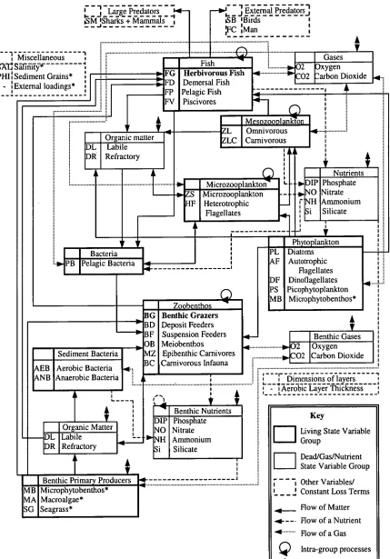
Figure 1.2: Biological and physical interactions between the components used in the Integrated Generic Bay Ecosystem Model IGBEM). A `*' indicates those components from the Port Phillip Bay Integrated Model, and those in bold are components built specifically for IGBEM, while the remainder are from the European Regional Seas Ecosystem Model II (Blackford and Radford 1995). The code for each component is given by its name.

- Large Predators ISMiSharks + Mammals

—V _JExternal Predators' ISB 'Birds :Man 'I Miscellaneous I PAV SWInit)7*- NI:Sediment Grains*

- :External loadings*

■ Fish

G Herbivorous Fish Demersal Fish IFD

IFP Pelagic Fish Piscivores

Gases 2 Oxygen 02 2arbon Dioxide

I Microzooplanktong Microzooplankton

I

J Heterotrophic Flagellates Nutrients DIP Phosphate NO Nitrate NH Ammonium Si Silicate

V

Benthic Primary Producers MB Microphytobenthos* MA Macroalgae* SG Seagrass*

411-

■••

-. _{Benthic Nutrients}

o

A

Z Z '

65 Phosphate Nitrate Ammonium Silicate Bacteria

PB Pelagic Bacteria

r

1 i Dimensions of layers

4

-I Aerobic Layer Thickness

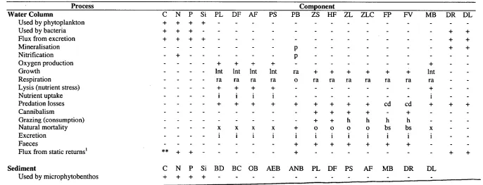
[image:42.559.85.514.151.766.2]

(43)

[image:43.834.75.761.242.505.2]

Table 1.2:

Level of detail used in the model formulation for each of the processes carried out in a standard run of the Integrated Generic Bay

Ecosystem Model. Component codes are as stated in Table 1.1 (except for C, N, P, Si which are Carbon, Nitrogen, Phosphorous and Silica

respectively). The symbols indicate the formulation used for each process as follows: activity; basal; constant (not dynamic); dynamic; DIN (epiphytic

growth) effect; search and handling times included; internal pool controls; light limitation; depth effect

(m);

nutrient effect; oxygen effect; performs

this physical activity; rest; starvation; temperature effect; crowding; assumed in formulation but not explicit; physical bottom stress effect; present (+);

absent (-). ** indicates that there is a flux of C from the static returns, but in the form of carbon dioxide.

Process Component

Water Column C N P Si PL DF AF PS PB ZS HF ZL ZLC FP FV MB DR DL

Used by phytoplankton + + + + - - -

Used by bacteria + + + + +

Flux from excretion Mineralisation Nitrification

+ + + +

+ - - p p - - -

+ + + +

Oxygen production + + + + - - +

Growth Int Int Int Int ra + + + + + + Int

Respiration ra ra ra ra o ra ra ra ra ra ra ra

Lysis (nutrient stress)

Nutrient uptake - - + i + i + i + i + i -

Predation losses - + + + + + + + + + cd cd + + +

Cannibalism

Grazing (consumption) - - - - + + + + + h + h h + h - -

Natural mortality x x x x + o o o o bs bs x

Excretion i i i i i i i i i i i i

Faeces + + + + + + +

Flux from static returns' ** ± • -i- - - + + +

Sediment C N P Si BD BC OB AEB ANB PL DF PS AF MB DR DL

(44)

Process Component

C N P Si BD BC OB AEB ANB PL DF PS AF MB DR DL

Used by bacteria + + + ontm ontm

Flux from excretion + + + + - - -

Mineralisation - p p -

Nitrification + - -

Denitrification + - - -

Oxygen production2 .. .. - - - -

Growth ot ot ot ra ra -

Respiration - ra ra ra otra2 otra2 -

Nutrient uptake - - - ontm ontm -

Predation losses + + + + +

Cannibalism _ _ + + - -

Grazing (consumption) - + + + -

Natural mortality ot ot ot + + + + + + +

Excretion - i i i i

Faeces _ _ + + +

Impact upon bioirrigation/bioturbation + + + -

Epibenthic C N P Si MZ BF BG MA SG FD FG DR DL

Used by macrophytes + + + -

Flux from excretion - - + +

Oxygen production + + + - - - - + +

Growth - + +

Respiration - - ot ot ot lntw lntw + +

Lysis (nutrient stress) - ra ra ra x x ra ra

Nutrient uptake - + + -

Predation losses - + + + + + cd cd + +

Cannibalism + - - +

Grazing (consumption) - + + + - h h -

Natural mortality _ _ _ ot ot ot by be bs bs

Excretion i i i an an i i

Faeces + + + + +

Flux from static returns' + +

Impact upon bioirrigation and bioturbation - + + + -

1. i.e. a % of the losses to fishing/seabirds/large predators

+ +

- + lnt2

ra i

(45)

[image:45.557.64.522.160.594.2]

The effects of model structure and complexity on the behaviour and performance of marine ecosystem models