ON OUTPUT FEEDBACK NONLINEAR MODEL PREDICTIVE CONTROL USING HIGH GAIN
OBSERVERS FOR A CLASS OF SYSTEMS
Lars Imsland∗,1 Rolf Findeisen∗∗ Eric Bullinger∗∗
Frank Allg¨ower∗∗,2 Bjarne A. Foss∗
∗
Department of Engineering Cybernetics, Norwegian University of Science and Technology, 7491 Trondheim, Norway,
{Lars.Imsland,Bjarne.Foss}@itk.ntnu.no
∗∗
Institute of Systems Theory in Engineering, University of Stuttgart, 70550 Stuttgart, Germany,
{findeise,bullinger,allgower}@ist.uni-stuttgart.de
Abstract: In recent years, nonlinear model predictive control schemes have been derived that guarantee stability of the closed loop under the assumption of full state information. However, only limited advances have been made with respect to output feedback in connection to nonlinear predictive control. Most of the existing approaches for output feedback nonlinear model predictive control do only guarantee local stability. Here we consider the combination of stabilizing instantaneous NMPC schemes with high gain observers. For a special MIMO system class we show that the closed loop is asymptotically stable, and that the output feedback NMPC scheme recovers the performance of the state feedback in the sense that the region of attraction and the trajectories of the state feedback scheme are recovered for a high gain observer with large enough gain and thus leading to semi-global/non-local results.
Keywords: Output Feedback Stabilization, Nonlinear Model Predictive Control, High Gain Observers
1. INTRODUCTION
Model predictive control for systems described by nonlinear ODEs (NMPC) is an area that has received considerable attention over the past years. Several schemes guaranteeing stability un-der state feedback exist, see for example (Mayne
et al., 2000; Allg¨ower et al., 1999; De Nicolao et al., 2000) for recent reviews.
Fewer results are available in the case when not all states are directly measured. A common approach is to design a state feedback NMPC and to use a state observer to obtain an estimate of the system states used in the NMPC. In this case, little can
1 This work was done while LI visited the IST 2 corresponding author
is available.
In this article we propose the use of high gain ob-servers in conjunction with instantaneous NMPC. For a special MIMO system class, the resulting control scheme does allow performance recovery of the state feedback controller if the observer gain is increased, i.e. the region of attraction and the rate of convergence of the output feedback scheme approach that of the state feedback scheme. To show stability, we will mainly use results on separation principles for the considered class of systems as described in (Atassi and Khalil, 1999), see also (Teel and Praly, 1995; Esfandiari and Khalil, 1987). There, it is shown that a high-gain observer, in combination with a globally bounded state feedback can, under certain conditions such as locally Lipschitz continuity of the state feed-back law, achieve recovery of asymptotic stability and performance.
The remainder of the paper is structured as fol-lows. In Section 2 we specify the considered class of systems. Section 3 states the NMPC schemes considered for state feedback. In Section 4 the high-gain observer for state estimation is outlined. Section 5 contains the main results for the result-ing closed loop system. These results are discussed in more detail in Section 6, and are illustrated with a simulation case study involving a mixed-culture bio-reactor with competition and external inhibition in Section 7.
2. SYSTEM CLASS
We consider nonlinear systems of dimensionr+l of the form
˙
x=Ax+Bφ(x, z, u) (1a) ˙
z=ψ(x, z, u) (1b)
y= ·
Cx z
¸
(1c)
where x(t) ∈ Rr and z(t) ∈ Rl are the state variables and y(t) ∈ Rp+l are the measured outputs. Notice that we assume that all states z are directly measured. The control input is assumed to be constrained, i.e. u(t) ∈ U ⊂ Rm andU satisfies the following Assumption:
Assumption 1. U ⊂Rmis compact and the origin is contained in the interior ofU.
Hence u is bounded and the equilibrium does satisfy the input constraint.
Ther×rmatrixA,r×pmatrixB and thep×r matrixChave the following form:
A= blockdiag [A1, A2, . . . Ap]
Ai=
0 1 0 ··· 0
0 0 1 ··· 0 ..
. ...
0··· 0 1 0··· ··· 0
ri×ri
B= blockdiag [B1, B2, . . . , Bp] Bi=
£
0 · · · 0 1¤T
ri×1
C= blockdiag [C1, C2, . . . , Cp] Ci=
£
1 0 · · · 0¤
1×ri,
i.e. the first part of the dynamics xconsists of p integrator chains, withr=r1+· · ·+rp.
Assumption 2. The functionsφ:Rr×Rl× U →
Rp and ψ : Rr
×Rl
× U → Rl are assumed to be locally Lipschitz in their arguments over the domain of interest with φ(0,0,0) = 0 and ψ(0,0,0) = 0. Additionally we assume, that φ is bounded inxeverywhere3.
One example of systems of this class are input affine nonlinear systems of the form
˙
ζ=f(ζ) +g(ζ)u, y=h(ζ)
with full (vector) relative degree (r1, r2, . . . , rp), that is, Pp
i=1ri = dimζ. Then, it is possible to find a coordinate transformation such that the system is described by (1a) and (1c), see (Isidori, 1985).
3. NONLINEAR MPC STATE FEEDBACK
The proposed output feedback controller consists of a suitable high gain observer to estimate the states and an instantaneous full state feedback NMPC controller. In the framework of predictive control, the input is defined by the solution of an open loop optimal control problem that has to be solved at all times. Here we assume that the input to the system is derived via the following NMPC open loop control problem:
State feedback NMPC open loop optimal control problem:
Solve min
¯
u(·)J(x(t), z(t),u(¯ ·)) (3) subject to:
˙¯
x=A¯x+Bφ(¯x,z,¯ u),¯ x(0) =¯ x(t) (4a) ˙¯
z=ψ(¯x,z,¯ u)¯ z(0) =¯ z(t) (4b) ¯
u(τ)∈U, τ∈[0, Tp] (4c)
(¯x(Tp),¯z(Tp))∈Ω (4d)
with the cost functional:
J(x(t), z(t),u(¯ ·)) := Z Tp
0
F(¯x(τ),z(τ),¯ u(τ))dτ¯
+E(¯x(Tp),z(T¯ p)). (5)
3 The assumption on global boundedness of φ in x is
The bar denotes internal controller variables and ¯
x(·) is the solution of (4a)-(4b) driven by the input ¯
u(·) : [0, Tp]→ U with initial condition x(t), z(t) at time t. The stage cost to be minimized over the control horizonTp is given by F(¯x,¯z,u). We¯ assume, thatF satisfies:
Assumption 3. F:Rr×Rl×U →Ris continuous in all arguments withF(0,0,0) = 0 andF(x, z, u)> cFk(x, z, u)k22 ∀(x, z, u)∈Rr×Rl× U,cF ∈R+.
The constraint (4d) in the NMPC open loop op-timal control problem forces the final predicted state at time τ =TP to lay in a terminal region denoted by Ω and is thus often called terminal region constraint. In the cost functional J, the deviation from the origin of the final predicted state is penalized by the final state penalty term E.
Notice, that for simplicity we only consider in-put constraints (besides the terminal state con-straint). An extension to more general cases is possible.
We denote the solution to the optimal control problem by ¯u⋆(
·;x(t), z(t)). The system input used is given by the “first” value of the instan-taneous solution of the open loop optimal control problem ¯u⋆(
·;x(t), z(t)):
u(x(t), z(t)) := ¯u⋆(τ= 0;x(t), z(t)). (6)
Several NMPC concepts that guarantee stabil-ity and that are similar to this setup have been proposed (Mayne and Michalska, 1990; Chen and Allg¨ower, 1998; Jadbabaie et al., 1999a), see (Mayne et al., 2000) for a review. Similar re-sults have also been obtained for the discrete time case (Meadows and Rawlings, 1993; De Nicolaoet al., 1996; Findeisen, 1997).
Under the assumption that Tp, E, F are suit-ably chosen (see for example (Chen and Allg¨ower, 1998; Jadbabaieet al., 1999a; Mayneet al., 2000)) the origin of the nominal closed–loop system with the input (6) is asymptotically stable and the region of attractionR ⊂Rr×Rlcontains the set of states for which the open loop optimal control problem has a solution.
We will assume that Tp, E, F are chosen such, that the state feedback defined via the NMPC open loop optimal control problem and (6) is locally Lipschitz and stabilizes the system, i.e. we assume that the following assumption holds:
Assumption 4. The instantaneous state feedback defined by u(x(t), z(t)) := ¯u⋆(τ = 0;x(t), z(t)) is locally Lipschitz in (x, z) and asymptotically sta-bilizes the system (1) with a region of attraction
R.
Remark 1. Notice that we assume an instanta-neous state feedback, i.e. the solution of the open
loop optimal control problem is available with no computational delay.
Remark 2. In general, the solution of an optimal control problem (and hence, the state feedback defined in Assumption 4) can be non-Lipschitz in the initial values. In (Jadbabaieet al., 1999b) it is noted that the control of anunconstrainedNMPC problem is continuous given that the minimum value of the cost function is attained, and that some regularity conditions onf,F andE, similar to those in this paper hold. Some results cerning the Lipschitz continuity of optimal con-trol problems have been reported (Hager, 1979; Dontchev and Hager, 1993). However the result-ing conditions are difficult to check and do only consider the Lipschitz continuity of the control law in terms of system parameters and not initial conditions.
4. USED HIGH GAIN OBSERVER
The proposed (partial state) observer is a high gain observer as in (Atassi and Khalil, 1999; Teel and Praly, 1995; Tornamb`e, 1992). It is of the following form:
˙ˆ
x=Aˆx+Bφ(ˆx, z, u) +H(yx−Cx) (7)ˆ whereH = blockdiag [H1, . . . , Hp],
HT i =
h
α(1i)/ǫ, α (i)
2 /ǫ2, . . . , α(ni)/ǫ ri
i
and theα(ji)s are such, that the roots of
sn+α(i) 1 s
n−1+
· · ·+α(n−i)1s+α (i)
n = 0, i= 1, . . ., p
are in the open left half plane.yxare the measure-ments of thexstates,yx=Cx. 1ǫ is the high-gain parameter, which can be seen as a time scaling for the observer dynamics (7).A,B,C andφare the same as in (1).
Remark 3. We only have to design an observer for the xstates of the integrator chain, since the z states are assumed to be measured directly.
5. OUTPUT FEEDBACK NMPC USING HIGH GAIN OBSERVERS
Now we are ready to state our main result, which follows from (Atassi and Khalil, 1999) and in part from (Teel and Praly, 1995). In short, we can claim recovery of performance and asymptotic stability (see Remark 4) of the origin if the parameterǫin the observer is chosen small enough (that is, the observer is fast enough).
and using the observed state ˆxfrom the observer (7) instead of x. Notice that the state feedback NMPC is assumed to asymptotically stabilize the system with a region of attraction R and that the value of the input is bounded, since the input constraint setU is compact.
Theorem 1. LetS be any compact set contained in the interior of R. Then there exists a (small enough) ǫ∗
> 0 such that for all 0 < ǫ ≤ ǫ∗ , the closed loop system is asymptotically stable with a region of attraction of at leastS. Further, the performance of the state feedback NMPC controller is recovered asǫdecreases.
Proof 1. The asymptotic stability follows directly from the proofs of Theorem 1, 2 and 4 in (Atassi and Khalil, 1999) under the given assumptions. Theorem 3 in (Atassi and Khalil, 1999) shows that the trajectories of the controlled system using the observed state in the controller, converge uniformly to the trajectories of the controlled system using the true state in the controller, as ǫ→0. Hence, forǫsmall enough, the trajectories (and hence the performance) of the state feedback NMPC are recovered.
In the following we briefly specify what is meant by recovery of performance.
Remark 4. [Trajectory convergence/performance recovery] Defineχo(t, ǫ) as the state of the system at time t using the output feedback NMPC con-troller withχo(0, ǫ) = (x(0), z(0)) as initial condi-tion and using ˆxfrom the observer (started with the initial condition ˆx(0)) instead ofxin the con-troller. Defineχs(t) as the state of the system at timet using the state feedback NMPC controller with χs(0, ǫ) = (x(0), z(0)) as initial condition. Then, for anyξ >0, there exists an ˜ǫ∗ such that for all 0< ǫ≤˜ǫ∗,
kχo(t, ǫ)−χs(t)k ≤ξ, ∀t >0. This trajectory convergence in ǫleads to what is meant by performance recovery and implies for example conformance to constraints, recovery of the region of attraction and rate of convergence.
If state constraints are included in the NMPC formulation, then we see that the state constraints are respected by the output feedback controller within any degree of accuracy by makingǫ small enough. However restrictive state constraints in the NMPC controller may lead to violation of the Lipschitz continuity condition on the controller, and hence are not included.
Remark 5.(Robustness). In the separation prin-ciple in (Atassi and Khalil, 1999), robustness to some modeling error in the observer (that is, in φ) is shown. In our case, it makes no sense to consider the observer model as incorrect, since we assume that we have perfect model knowledge in
the NMPC controller. However, it indicates that the observer structure has some robustness prop-erties (see (Teel and Praly, 1995, Lemma 2.4)).
6. DISCUSSION
The result in Section 5 is based on the assump-tion that the NMPC controller is time contin-uous/instantaneous. In a real application, it is of course not possible to solve the nonlinear op-timization problem instantaneously. Instead, it typically will be solved only at some sampling instants. The first part of the computed control is then applied to the system, until the next sam-pling instant. Further, some time is needed to compute the optimal solution of the optimization problem, thus the computed control to some de-gree is based on old information, introducing delay in the closed loop.
In a transient phase, due to the peaking phe-nomenon, the observed state may be outside the region where the NMPC optimization problem has a feasible solution. In this case the input should be assigned some fallback value. The high gain observer structure and the results of (Atassi and Khalil, 1999) ensure that ǫ can be chosen small enough so that the observer state converges to the true state before the true state leaves the re-gion of attraction (and hence the feasibility area) of the NMPC controller. This follows from the assumption of bounded controls (Esfandiari and Khalil, 1992).
7. EXAMPLE
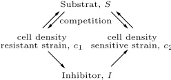
[image:4.612.349.473.598.656.2]To show recovery of performance we consider the control of a continuous mixed culture bioreactor as presented in (Hoo and Kantor, 1986). The model considered describes the dynamics of a culture of two cell strains, in the following called species 1 and 2, that have different sensitivity to an external growth-inhibiting agent. The interac-tions of the two cell populainterac-tions is illustrated in Figure 1. The cell density of the inhibitor resistant
resistant strain,c1
cell density cell density
Substrat,S
sensitive strain,c2
Inhibitor,I
competition
Fig. 1. Strain/inhibitor interactions.
strain is denoted by c1, the cell density of the
inhibitor sensitive strain is denoted with c2 and
dc1
dt =µ1(S)c1−c1u1, dc2
dt =µ2(S, I)c2−c2u1, dI
dt =−pc1I+u2−Iu1.
The inputs are the dilution rateu1 =D and the
inhibitor addition rate u2 = DIf, with If being the inhibitor inlet concentration. The deactivation constant of the inhibitor for species 2 is denoted by p. µ1(S) and µ2(S, I) are the specific growth
rates given by:
µ1(S) = µ1,MS
K+S, µ2(S, I) = µ2,MS K+S
KI KI+I
.
whereK,KI,µ1,M andµ2,M are constant param-eters. The substrate concentration is given by:
S=Sf− c1
Y1 −
c2
Y2
.
Here Y1, Y2 are the yields of the species and Sf is the substrate inlet concentration. The control objective is to stabilize the steady state given by c1s = 0.016g/l, c2s = 0.06g/l, Is = 0.005g/l. We will use the output-feedback NMPC scheme as outlined in the previous sections to achieve this. If we use
yT = [lnc1 c2, c1]
as measured outputs and if we make the following coordinate transformation
x1= ln
c1
c2
, x2=µ1(S)−µ2(S, I), z=c1
the transformed system is of the model class as-sumed in Section 2:
˙ x1=x2,
˙
x2=φ(x1, x2, z, u1, u2),
˙
z=ψ(x1, x2, z, u1, u2).
As NMPC scheme we use the so called quasi-infinite horizon NMPC strategy as presented in (Chen and Allg¨ower, 1998) with the sampling time set to zero. As cost F we use the quadratic deviation of the states and the inputs in the new coordinates from their steady state values. For simplicity unit weights on all states and inputs are considered. The horizonTpwas set to 20hr. A quadratic upper boundE on the infinite horizon cost and a terminal region Ω that satisfy the assumptions of (Chen and Allg¨ower, 1998) and with this the assumptions made in Section 3 are calculated using LMI/PLDI-techniques (Boyd et al., 1994). The piecewise linear differential in-clusion (PLDI) representing the dynamics in a neighborhood of the origin was found using the methods described in (Slupphauget al., 2000). The statesx1andx2are estimated from the
mea-surements ofx1 andzvia a high gain observer as
described in Section 4. The parametersα1andα2
are chosen toα1= √
2,α2= 1. To show the
recov-ery of performance we consider different values of the high-gain parameterǫof the observer. Notice, that in real applications the value of ǫ should not be decreased to much, since there is always a trade off between the performance recovery and the robustness to noise and modeling errors. For all cases the observer is started with the correct values for x1 and x3 (since they can be directly
obtained from the measurements), whereas x2 is
assumed unknown and initialized with the steady state value. Figure 2 shows closed-loop system tra-jectories for different observer gains 1ǫ in compari-son to a state feedback NMPC controller (using no high gain observer for state recovery). As can be
0.1 0.11 0.12 0.13 0.14 0.15 0.16
0.04 0.045 0.05 0.055 0.06
c2
[g/l]
c1 [g/l]
ss
[image:5.612.331.500.240.372.2]statefeedback eps=1 eps=10 eps=100
Fig. 2. Phase plot ofc1andc2(SS. . . steady state)
seen, the higher the observer gain gets, the more performance is recovered by the output feedback controller, i.e. the trajectories tend towards the “optimal” state feedback ones. Figure 3 exempli-fies the time behavior of the inhibitor concentra-tion I (related to the unmeasured state x2) and
the inhibitor addition rate DIF (input u2) for
different values ofǫ. Additionally, we plot the real
0 5 10 15 20 25 30 35 40 45 50
3 3.5 4 4.5 5
x 10−3
I [g/l]
0 5 10 15 20 25 30 35 40 45 50
2 2.1 2.2
x 10−3
D*If [g/l hr]
0 5 10 15 20 25 30 35 40 45 50
0 0.1 0.2
resulting cost
time [hr] statefeedback
eps=1 eps=10 eps=100
Fig. 3. Trajectories ofI, u1 and summed up cost
[image:5.612.310.520.510.682.2]cost. The cost of the output feedback controller approaches the cost of the state feedback con-troller for decreasing ǫ, which shows the recovery of performance.
Notice, that we use relatively low gains of the observer, meaning thatǫis large. Higher observer gains can lead to problems in case of measurement noise. This is one of the main limitations of using high gain observers for state estimation. We do not go into details here. The given example under-pins the derived results on performance recovery for the high-gain observer based NMPC strategy.
8. CONCLUSIONS
Nonlinear model predictive control has received considerable attention during the recent years. However no significant progress with respect to the output feedback case has been made. The ex-isting solutions are either of local nature (Scokaert
et al., 1997; Magni et al., 1998) or difficult to implement (Michalska and Mayne, 1995). In this paper we have outlined, that using results from (Atassi and Khalil, 1999), “semi-global” sta-bility results on a bounded region of attraction and recovery of performance can be achieved uti-lizing NMPC and a suited high gain observer for a class of systems. The price to pay is that one has to assume that the NMPC control law is local Lipschitz in the states over the domain of interest and that only systems with “directly measurable internal dynamics” can be considered. However, in practical problems the locally Lipschitz assump-tion is often not a significant problem. Addiassump-tion- Addition-ally, one should notice the inherent problem of high gain observers with respect to measurement noise. The given result must be seen as a first step towards the development of a practical relevant output feedback NMPC scheme.
9. REFERENCES
Allg¨ower, F., T.A. Badgwell, J.S. Qin, J.B. Rawlings and S.J. Wright (1999). Nonlinear predictive con-trol and moving horizon estimation – An introduc-tory overview. In:Advances in Control, Highlights of ECC’99(P. M. Frank, Ed.). pp. 391–449. Springer. Atassi, A.N. and H. Khalil (1999). A separation principle
for the stabilization of a class of nonlinear systems.
IEEE Trans. Automat. Contr.44(9), 1672–1687. Boyd, S., L. El Ghaoui, E. Feron and V. Balakishnan
(1994). Linear Matrix Inequalities in System and Control Theory. SIAM. Philadelphia.
Chen, H. and F. Allg¨ower (1998). Nonlinear model pre-dictive control schemes with guaranteed stability. In:
Nonlinear Model Based Process Control(R. Berber and C. Kravaris, Eds.). Kluwer Academic Publishers, Dodrecht. pp. 465–494.
De Nicolao, G., L. Magni and R. Scattolini (1996). Stabi-lizing nonlinear receding horizon control via a non-quadratic terminal state penalty. In:Symposium on Control, Optimization and Supervision, CESA’96 IMACS Multiconference. Lille. pp. 185–187.
De Nicolao, G., L. Magni and R. Scattolini (2000). Stability and robustness of nonlinear receding horizon control. In: Nonlinear Predictive Control (F. Allg¨ower and A. Zheng, Eds.). Birkh¨auser. pp. 3–23.
Dontchev, A. and W. Hager (1993). Lipschitzian stability in nonlinear control and optimization.SIAM J. Con-trol Optim.31(3), 569–603.
Esfandiari, F. and H.. Khalil (1987). Observer-based design of uncertain systems: recovering state feedback ro-bustness under matching conditions. In:Proc. of the 25th Anual Allerton Conf. on Comunication, Con-trol, and Computing. Monticello, IL. pp. 97–106. Esfandiari, F. and H. Khalil (1992). Output feedback
sta-bilization of fully linearizable systems.Int. J. Contr.
56(5), 1007–1037.
Findeisen, R. (1997). Suboptimal nonlinear model predic-tive control. Master’s thesis. University of Wisconsin– Madison.
Hager, W.E. (1979). Lipschitz continuity for constrained processes.SIAM J. Contr. Optim.17(3), 321–338. Hoo, K. A. and J. C. Kantor (1986). Global linearization
and control of a mixed culture bioreactor with compe-tition and external inhibition.Math. Biosci.82, 43– 62.
Isidori, A. (1985).Nonlinear Control Systems: An Intro-duction. Springer-Verlag. Berlin.
Jadbabaie, A., J. Yu and J. Hauser (1999a). Stabilizing re-ceding horizon control of nonlinear systems: A control Lyapunov approach. In:Proc. Amer. Contr. Conf.. ACC. San Diego. pp. 1535–1539.
Jadbabaie, A., J. Yu and J. Hauser (1999b). Unconstrained receding horizon control of nonlinear systems. In:
Proc. 38th IEEE Conf. Decision Contr.. San Diego. pp. 3376–3381.
Magni, L., D. De Nicolao and R. Scattolini (1998). Out-put feedback receding-horizon control of discrete-time nonlinear systems. In:Preprints of the 4th Nonlin-ear Control Systems Design Symposium 1998 - NOL-COS’98. IFAC. pp. 422–427.
Mayne, D.Q. and H. Michalska (1990). Receding horizon control of nonlinear systems.IEEE Trans. Automat. Contr.35(7), 814–824.
Mayne, D.Q., J.B. Rawlings, C.V. Rao and P.O.M. Scokaert (2000). Constrained model predictive con-trol: stability and optimality.Automatica26(6), 789– 814.
Meadows, E.S. and J.B. Rawlings (1993). Receding horizon control with an infinite horizon. In: Proc. Amer. Contr. Conf.. San Francisco. pp. 2926–2930. Michalska, H. and D.Q. Mayne (1993). Robust
reced-ing horizon control of constrained nonlinear systems.
IEEE Trans. Automat. Contr. AC-38(11), 1623–
1633.
Michalska, H. and D.Q. Mayne (1995). Moving horizon observers and observer-based control. IEEE Trans. Automat. Contr.40(6), 995–1006.
Scokaert, P.O.M., J.B. Rawlings and E.S. Meadows (1997). Discrete-time stability with perturbations: Application to model predictive control.Automatica
33(3), 463–470.
Slupphaug, O., L. Imsland and B. Foss (2000). Uncertainty modelling and robust output feedback control of non-linear discrete systems: a mathematical programming approach.International Journal of Robust and Non-linear Control10(13), 1129–1152.
Teel, A. and L. Praly (1995). Tools for semiglobal stabi-lization by partial state and output feedback.SIAM J. Contr. Optim.33(5), 1443–1488.