Polynomial Selection for the
Number Field Sieve
Integer Factorisation Algorithrn
Brian
.
Antony Murphy
A Tf!CSIS SUBMITTED FOR THE DECREE OF DOCTOR OF PHILOSOPHY OF THE AUSTRALlAN NATIONAL lJ[:!IVERSITY
.
1Declaration
Except where otherwise indicated, this thesis is my own original work.
111
Acknowledgments
I have been afforded the rare opportunity of working as a student of Richard Brent. Over the last three years, Richard has provided encouragement, guidance and sugges-tions from which I have learnt a great deal and for which I am extremely gratefuL Richard was also considerate enough to take up a chair in Computing Science at Ox-ford University in 1998. That gave me an excuse to visit him there, about which I will say more later.
I also owe a great deal to Peter Montgomery ( CWI, Amsterdam and Microsoft Research, USA). Peter's influence on current research in this field is far more extensive than most people realise. I have had the benefit of many long discussions with Peter, and a great deal of patient instruction from him. Several key sections of this thesis are developed from ideas originating from discussions with Peter.
My research experience has been enriched and broadened through close collab-oration with the Computational Number Theory and Data Security group at CWI in Amsterdam. I thank Herman te Riele, the head of the group, for fostering that collaboration and supporting two visits by me to CWI.
I am also grateful to Arjen Lenstra (Citibank, USA) and John Pollard. Both gentle-men perused early versions of some of the work contained herein and provided valuable comments and suggestions. My thesis would contain many errors and inconsistencies but for some close reading by Mike Newman (ANU) and Adam Hall.
Funding is crucial to research, and I express thanks to all those who have funded mine. The CRC for Advanced Computational Systems (ACSys) funded the first year of my PhD and provided professional development and travel support there_?,fter. The second and third years of my PhD were funded by an Australian Postgraduate Award. My second and third years were also funded partially by the Defence Science and Technology Organisation (DSTO). I am particularly grateful to Richard Taylor at DSTO for his support and input to my research.
I was very fortunate to be able to spend close to six months visiting Richard Brent at Oxford. I thank Richard, the Oxford -University Computing Laboratory, and the providers of the Australian Bicentennial Sc~ol3:Iship ,fm supporting that visit. This was one of most valuable experiences of my PhD.
Let me turn to some personal thanks. Several people have been unfortunate enough to share a house with me in Canberra or Oxford over the past three years. To those of you who are still talking to me, thank you for some wonderful times. I draw particular attention to those with excellent squash or culinary skills.
I need to acknowledge my good friend Rachel Thomas in Perth, because she will be cross if I don't.
.
IVfront of the screen have also been a large part of my PhD experience. Thank you to anyone who made them bearable.
V
Abstract
List of Symbols
The following symbols are used in this thesis without further definition.
the (rational) integers
Zn
the integers modulo nthe rational numbers
the real numbers
the complex numbers
Z[x]
the set of polynomials inx with integer coefficients
(Q(
a) the number field defined by a, with a E C satisfyingf (a)
=
0 for somef
EZ[x]
of degreed
Z[a) the ring of Z-linear combinations of {1, a, .. . , ad- l} with a as above
the ring of (algebraic) integers of
(Q(
a)(;) the Legendre symbol for n mod q
ordpn the exponent of the largest power of p dividing n
<p(
n) Euler's phi functionlr
J
the floor of r E IR.
.
Contents
Declaration
Acknowledgments
Abstract
List of Symbols
1 Introduction
1.1 Integer Factorisation and Public-Key Cryptography
1.1.1 The RSA Public-Key Cryptosystem
1.1.2 Other Public-Key Systems . . . .
1.2 Factorisation of General Integers . . . . 1.2.1 Factorisation by Congruent Squares
1.2.2 Congruent Squares from Smooth Polynomial Values 1.2.3 Complexity Estimates . . . .
1.2.4 The RSA Factorisation Challenge .
1.3 The Number Field Sieve Briefly . . . . 1.3.1 The Algorithm . . . .
1.3.2 The Number Field Sieve for Discrete Logarithms
1.3.3 The Polynomial Selection Problem
1.4 Contribution of the Thesis .
1.4.1 Polynomial Yield . . 1.4.2 Polynomial Selection
1.4.3 Polynomials for Record Factorisations
1.5 Outline of the Thesis . . . .
2 Background
2.1 The Number Field Sieve
Outline . . . 2.1.1
2.1.2
2.1.3
Congruent Squares from Smooth Polynomial Values
The Sieving Step . . . .
X
2.1.4 The Matrix Step ..
2.1.5 The Square Root Algorithm .
2.2 Smooth Integers . . . .
2.2.1 Smooth Integers Generally
2.2.2 Smooth Integers and the Number Field Sieve
2.3 Polynomial Selection . .
2.3.1 Non-linear Methods
2.3.2 The Base-m Method
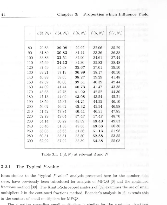
3 Properties which Influence Yield 3.1 Size . . . . . . . .
3.2 Root Properties . . . .
3.3
3.2.1 The Typical F-value ,
3.2.2 Estimating contp(
v)
3.2.3 Quantifying Root Properties
3.2.4 Root Properties and d Summary .
4 Modelling Yield
4.1 Yield as a Function of Root Properties
4.1.1 In Theory: Boender's Yield Estimation
4.1.2 Full Yield as a Function of a
4.1.3 lLP-Yield as a Function of a
4.1.4 2LP-Yield as a Function of a
4.1.5 In Practice: Sieving Experiments
4.2 Modelling Yield . . . .
4.3
4.2.1 Actual Yield
4.2.2 Estimating Yield 4.2.3 Examples .
4.2.4 Polynomials for Larger N
Summary ..
5 Finding Good Polynomials
5.1 Generating Good Polynomials .
5.1.1 Non-skewed Polynomials .
5.1.2 Skewed Polynomials . .
5.2 Isolating the Best Polynomials
5.2.1 Non-skewed Polynomials .
5.2.2 Skewed Polynomials 5.3 Summary . . . .
Contents 28 29 30 30 32
36
36
39 41 42 43 44 45 48 50 54 57 58 5860
61
6466
68
68
71 71 7374
7778
78
82 85Contents
6 Polynomials for RSA Factorisations
6.1 RSA-130 . . . .
6.1.1 The Fifteen Candidate Polynomials
6.1.2 On the Reliability of IE . . . 6.1.3 Eighteen Different Candidates .
6.1.4 Good Polynomials for RSA-130
6.1.5 Some Timing Considerations
6.2 RSA-140 . . . · . . . . 6.2.1 Non-skewed Polynomials . . . .
6.2.2 Skewed Polynomials - Local Considerations
6.2.3 Skewed Polynomials - Global Considerations 6.2.4 Some Timing Considerations
6.3 RSA-155 . .. . . .
6.3.1 Local Considerations . . . . . 6.3.2 Global Considerations . . . . 6.3.3 Some Timing Considerations
6.4 Summary . . . . 6.4.1 RSA-130 . 6.4.2 RSA-140 .
6.4.3 RSA-155 .
7 Conclusions and Further Work
7 .1 Con cl us ions .
7.2 Further Work . . . . .
A Appendix to Chapter 4
B Appendix to Chapter 6
B.l RSA-130 Polynomials
B.2 RSA-140 Polynomials
B.3 RSA-155 Polynomials
.
XI 8990
91 9294
95 9798
98
99
. 101. 102
. 102 102 . 104
107 . 110 110 110
111
113 113
. 113
115
Chapter 1
Introduction
Throughout life, and in particular throughout this thesis, N is a large integer requiring factorisation.
Some integers N require factorisation simply because they're large and interesting. Some require factorisation because, as well as being large and interesting, they're important cryptographically. We are concerned with factorising integers of the latter kind.
The most commonly used public-key cryptosystem is the RSA system. The security of RSA relies on certain large N being difficult to factorise. The best measure of the level of security offered by RSA is our ability to factorise such N.
Asymptotically and in practice, the fastest algorithm for factorising these integers is the number field sieve. The speed at which the number field sieve factorises N is determined by the supply of smooth integers (integers with no large prime factors) of a particular form. Given a certain pair of polynomials
f
1(x), f
2(x)
E.
Z[x)
each irreducible overQ
and of degree di for i=
1, 2, we use the homogeneous polynomials Fi ( x, y)=
ydiJi (
x / y). We search for coprime integer pairs a, b at which both F1 ( a, b) andF2 (
a,b)
are smooth. This search is the rate determining step in factorisingN
using the number field sieve.The area in which the number field sieve has had the greatest capacity for im-provement is in the selection of these polynomials. "Better" polynomials are ones which produce more smooth values. We cal} th~ problem of choosing better number field sieve polynomials the polynomial selection problem.
Motivated by both assessing and compromising the security of RSA and similar ;· systems, we consider in this thesis the polynomial selection problem for the number field sieve. The improvements given here were used to set a new record for factorisation of "general" N, by factorising the 140 digit RSA modulus RSA-140. At the time of writing, our improvements are also being used to factorise a 512 bit (155 digit) RSA modulus RSA-155.
In this chapter we introduce the polynomial selection problem. In Section 1.1 we consider the cryptographic context of the problem. In Section 1.2 we introduce the
2 Chapter 1: Introduction
strategy for factorising integers like RSA moduli. In Section 1.3 we outline very briefly the number field sieve, and focus on the polynomial selection problem. We are then in
a position in Section 1.4 to outline the contribution of this thesis, and in Section 1.5
to outline the thesis itself.
1.1
Integer Factorisation and Public-Key
Cryptography
Public-key cryptography [28] is a crucial aspect of modern communication networks.
Its aim is to ensure that communications over networks are secure.
Most public-key cryptosystems rely for their security on certain number-theoretic problems being intractable. By a large margin, the most commonly used form of
public-key cryptography is the RSA cryptosystem. RSA, and some other systems like
it, rely for their security on the problem of integer factorisation. Most other
public-key cryptosystems in use rely for their security on instances of the discrete logarithm
problem. Our results also affect some of these systems.
Next we describe the RSA cryptosystem. We also mention some alternative
public-key cryptosystems relying on the discrete logarithm problem. Our treatment is very
brief. A good survey of public-key cryptosystems, from the perspective of their und
er-lying number theoretic problem, is [79].
1.1.1
The RSA Public-Key Cryptosystem
In the RSA public-key cryptosystem [68] the public/private-key pair is generated from
two distinct large primes p, q of approximately the same size (in fact, they are usually
the same number of bits). Let N
=
pq. Choose e E Z coprime to <p(N)=
(p- l)(q-l)
and, using for example the extended Euclidean algorithm, computed _
e-1 modcp(N
).
The public-key is then the pair ( e, N) and the private-key is d. Encryption of the message block M occurs by computing
C _ Me mod N .
Decryption occurs by computing
Clearly, factorising N suffices to compromise the security of the system. Also,
factorising
N
is equivalent to factorisingcp(
N)
(see for example [11]). Whether thesecurity of RSA is equivalent to factorising N is an open problem. For the paranoid,
there are versions of RSA whose security is provably "almost" equivalent to factorising
·,
•
1.1 Integer Factorisation and Public-Key Cryptography 3
For practical purposes, RSA depends for its security on the difficulty of factorising N , the RSA modulus. Hence, the level of security provided by the system depends on our ability to factorise RSA moduli. Current recommendations of modulus length of course depend on the level of security desired. The minimum recommended length for financial and government communications requiring a high level of security is 1024 bits (319 digits). However, 512 bit moduli have been and still are commonly used. For example, 512 bits is the default length on certain Internet browsers, and therefore
such moduli protect a large portion of electronic commerce conducted over the Internet. Adi Shamir estimates that 512 bit RSA moduli protect approximately 95
%
of Internet electronic commerce(70)
.
1.1.2
Other Public~Key Systems
After integer factorisation, the most common problem on which the security of public-key cryptosystems is based is the discrete logarithm problem. Let G be a finite group. Without loss of generality we can assume G is cyclic, with generator g. Given a E G, the discrete logarithm problem in
G
is to compute x such thatSeveral cryptographic protocols rely on the discrete logarithm problem for their security, for example the Diffie/Hellman key exchange protocol [28), ElGamal [31], and elliptic curve systems [38].
The most desirable groups
G
for cryptographic purposes are the ones for which• the group multiplication law can be implemented efficiently, and
• the discrete logarithm problem in
G
is believed to be difficult.Two types of group have emerged in practice as satisfying these requirements; the multiplicative group of a finite field and the group of points on an elliptic curve over a finite field. We denote the first type by
GF(q)*
forq
=
pn
, p
prime, and the secondE( q). In both cases, q will usually be either p for odd p, or 2n with n
>
l.There is an analogous version of the number field sieve for factorisation which com-putes discrete logarithms in some groups of the Jirst type,
GF(q)*
·
.
Our improvementsto the number field sieve for factorisation carry over to this version, and so have an impact on the security of systems relying on these instances of the discrete logarithm problem. We discuss this after giving more details on the number field sieve.
It is significant from the point of view of the security of elliptic curve cryptosystems
4 Chapter 1: Introduction
1.2
Factorisation of General Integers
We focus now on factorisation methods relevant to cryptographic applications.
Not all integers of a given size are equally difficult to factorise. Some are trivial, and some are of a form that makes them susceptible to attack by special methods. In particular, the elliptic curve method [50), [10), and the Pollard-rho method [62] find "small" factors particularly well. The Pollard p - l method [61] succeeds in finding factors p for which p - l contains no large prime factors. For security, RSA moduli
need to be integers which are amongst the most difficult to factorise. That is, they need to be integers not susceptible to attack because of their particular form. We refer to integers with no helpful special form as general integers. RSA moduli, integers
N=pq
for primes p and q which are both "large" and not far from
-/N,
lie amongst the general integers.A family of algorithms has been developed for factorisation of general integers. The family is characterised by the factorisation strategy adopted by its members.
The number field sieve is the newest and best performing member of the family. Its
immediate predecessor is an algorithm called the multiple polynomial quadratic sieve (MPQS) [65], [7 4]. Several impressive factorisations of RSA moduli were performed
using MPQS before the number field sieve came into being. By way of background to the number field sieve we now explain the factorisation strategy of algorithms in the family, concentrating on MPQS and the number field sieve. For a more thorough background on factorisation algorithms the reader should refer to, for example, [67].
1.2
.
1
Factorisation
by
Congruent Squares
Long before the introduction of the RSA cryptosystem, Fermat posed the forerunner to the modern strategy. He noted that if positive integers
x
and y can be found for whichN
=
x2 - y2 .then a non-trivial factorisation of N follows immediately as the product
(x-y)(x+y).
The task then is to find x and y, that is, to find the representation of N as a difference
.of two squares. The definite article is used advisedly, every odd N which is a product of I
two prime factors has a unique representation as a difference of two squares. Therein lies a problem however; if 1'1 is large then finding the unique pair
(x,
y)
becomes difficult.An improvement usually attributed to Kraithcik [43] partly overcomes this problem.
1.2 Factorisation of General Integers 5
multiples of
N,
so there should be many representations for which to search. Hence,we now require integers x and y such that
x2 - y2 mod N.
(1.1)
That is, we require two congruent squares mod N. The trade-off is that we are no
longer guaranteed that the representation will produce a non-trivial factorisation of
N. We are guaranteed that Nl(x
-
y)(x
+
y),
from which we may hope that1
< gcd (
x±
y)
<
N.(1.2)
If for example,
N
=
pq and both p and q div1dex+
y
then(1.2)
will not hold. Howeverit is simple to show that amongst a sample of representations
(1.1)
we can expect(1.2)
to hold in at least one half of the cases. Hence we say that given a representation as
in
(1.1)
, we get a non
-trivial factor ofN
as in(1.2),
with probability at least one half.If
N
is an RSA modulus then this probability is exactly one half. In practice, findingmany representations
(1.1)
requires only trivially more effort than finding just one, sothis does not present an obstacle.
Despite the fact that it is simple, finding two congruent squares mod
N
becomes the strategy for factorising large general integers. Both MPQS and the number fieldsieve adopt this strategy. The question now becomes how to construct the congruent
squares.
lo2.2
Congruent Squares from Smooth Polynomial Values
Congruent squares are constructed from so-called B-smooth integers.
Definition 1.2.1 An integer is B -smooth if its largest prime factor is at most B .
If the precise value of
B
is immaterial we refer to these simply as smooth integers.There is a well known procedure for constructing squares from many smooth
inte-gers. Let 1r(B) denote the number of primes less than B. Suppose we collect K
>
1r(B)integers which are B-smooth. By some lirrear algebra modulo 2, we can be guaranteed
to _find a subset of these
K
integers the proquct: over-which is a square.How does this work? Let the smooth integers we collect be Vi for i
=
1, ... ,K.
We record the factorisation of each vi over the primes at most B in an exponent vectorvi of length 1r(B). The j-th entry of vi is 1 when the j-th prime appears to an odd
exponent in Vi, and O otherwise. That is, vi records the square-free portion of Vi, with
ones denoting the "square-free primes" in Vi. Now we find a subset S of the vi's which
"pairs-up" the square-free primes appearing throughout the primes Vi
E
S
.
How? We form a matrix over Z2 listing the vi for i=
1, .. . , K as rows. Since K>
1r(B), the number of columns, there is guaranteed to be a linear dependency, modulo 2, amongst6 Chapter 1: Introduction
rows vi which contribute to the dependency. The product over S is then guaranteed to be a square, since all the square-free primes are "paired-up" across the product.
Hence, from sufficiently many smooth integers, we can construct a square integer after
some linear algebra modulo 2. In practice, N is very large and therefore so is the
corresponding matrix ( typically there are millions of rows and columns).
Recall now that, more than just constructing squares, we are required to construct
congruent squares modulo N. To ensure that this will be the case on collection of
smooth integers, we require the smooth integers to be of a special form. In particular,
we require them to be values taken by certain polynomials. For the number field sieve
the mechanism by which we are guaranteed to get congruent squares from smooth
polynomial values is explained in Chapter 2. For now it suffices to know that both
MPQS and the number field sieve proceed by constructing congruent squares modulo
N, and that this occurs by collection of sufficiently many smooth values of certain
polynomials.
In MPQS, we collect smooth values of certain quadratic polynomials. The num -ber field sieve is more complicated, because there we collect smooth values of pairs
of polynomials. For example, often one polynomial will be quintic whilst the other
is linear. In both MPQS and the number field sieve, the collection of these smooth
values is overwhelmingly the most time consuming stage of the process. This stage is
called sieving. Other stages are complicated and time consuming too - for example a
large matrix requires elimination modulo 2 - but sieving dominates the run-time of the
algorithms. The polynomial selection problem for the number field sieve involves
re-ducing the sieving effort required by choosing polynomials which produce many smooth values.
1.2.3
Complexity
Estimates
We now consider the relationship between the collection of smooth polynomial values
and the run-time of the algorithms. The asymptotic complexity analyses of both
MPQS and the number field sieve are tied to the appearance of smooth integers in
the context of each algorithm. The results of these analyses give an intuitive picture
of where the asymptotic advantage of the number fiel_d sieve lies,"and what should be
exploited to best leverage this advantage in practice.
The following function is central to the analysis. Suppose we have real variables
1v, w with O
<
v<
l . Let the £-function be given byLx[v,
w]
=
exp [(w
+
o(l)) (log xt(log log x)1-
v)
J
.
The more important variable is
v.
Think of the £-function as interpolating ( alo:ngv)
between polynomial and exponential functions of log x. Indeed, Lx[l
,
w]
=
xw+o(l)and Lx[O,
w]
=
(log x)w+o(l). The value ofw
is not immaterial, but makes a difference'
I
1.2 Factorisation of General Integers 7
N Date Algorithm Effort (MY) Ref.
RSA-100 Apr 91 MPQS 7 N/A
RSA-110 Apr 92 MPQS 75 [29] RSA-120 June 93 MPQS 835 [25] RSA-129 Apr 94 MPQS 5000 [2] RSA-130 Apr 96 NFS 1000 [23] RSA-140 Feb 99 NFS 2000 (16] RSA-155 Sept 99? NFS
·
<
10000Table 1.1: RSA Challenge records
Algorithms in the "congruent squares" family typically have heuristic asymptotic
run-times described by the L-function. Heuristically, the time taken by MPQS to factor N is
LN[l/2
,
1] as N -+ oo. In fact, all general factorisation algorithms precedingMPQS also have asymptotic run-time at best
LN[l/2,
c] for some c>
1. The numberfield sieve however, has asymptotic run-time
LN[l/3,
(64/9)113] .The appearance of v
=
l/3 is exciting. It brings the number field sieve significantlycloser to a polynomial-time algorithm than its predecessors. We explore this issue
in Chapter 2. It is worth noting now that the reason the number field sieve defeats
other algorithms asymptotically is that the integers it requires to be smooth are much
smaller asymptotically than those of other algorithms. That is, asymptotically, the
number field sieve guarantees a much better supply of smooth polynomial values.
1.2.4 The RSA Factorisation Challenge
The number field sieve is clearly the state-of-the-art asymptotically, but what is the
.
situation in practice? State-of-the-art for general integer factorisation in practice is
measured by progress through the RSA-·Factorisation Challenge. The RSA
Factorisa-tion Challenge is a list of genuine RSA mod ~li. 'fhe -Chal-lenge is administered by RSA
Laboratories [69] precisely to encourage and keep track of factorisation research.
The challenge numbers begin at length 100 digits, and there is one at every length
110, 120, ... , 500 digits. There are also moduli of length 155 digits (512 bits), 232
digits (768 bits), 309 digits (1024 bits) and 617 digits (2048 bits).
Table 1.1 shows progress through the list, including the record RSA-140
factorisa-tion and the impending RSA-155 record.
The MIPS-years figures for the effort required to factorise each number are very approximate. For RSA-130 and RSA-140 the figures are a little misleading. Lower, but
[image:20.786.114.618.135.389.2]MIPS-8 Chapter 1: Introduction
years respectively. The prediction for RSA-155 is based on extrapolation from the 2000
MIPS-years figure for RSA-140. We re-visit this estimate in Chapter 6.
The integers of most interest to us are 129, 130, 140 and
RSA-155. RSA-129 is not formally part of the RSA Challenge list, it is included here
for illustration purposes only. It was set as a challenge in the August 1977 edition of
Scientific American. Accompanying the challenge was the now infamous claim that the
RSA-129 modulus would be secure for 40 quadrillion years. The RSA-129 factorisation is the last record set using MPQS. The RSA-130 record is significant because it is the
first set using the number field sieve. Notice the decrease in estimated MIPS-years
effort from RSA-129 to RSA-130. Notice also that the RSA-140 record, even with
the conservative estimate of effort, was still set with less than half the effort used for
RSA-129.
These figures refer only to the effort spent on the sieving stage of each algorithm;
the stage during which smooth polynomial values are collected. Certainly this is the
stage that requires the most effort, but particularly with the number field sieve, other stages are also complicated and time consuming.
1.3
The Number Field Sieve Briefly
In this section we outline very briefly the steps involved in the number field sieve.
More details are given in Chapter 2. We also note the existence of an analogue of the
number field sieve for computing discrete logarithms in Zp-l· Finally we focus on the
polynomial selection problem.
The number field sieve was developed from ideas of Pollard
[63)
in 1988.It
wasinitially formulated to apply to integers of a special form (for which the polynomial
selection step is easy). This earlier version is now referred to as the special number
field sieve. The special number field sieve had early success with the factorisation of
the ninth Fermat number
Fg
[47]. Since the polynomial selection step is easy in thespecial number field sieve, that is, an obvious pair of exceptionally good polynomials
is known in advance for N , its asymptotic run-time is only
.For completeness we note that the largest integer factorised by the special number field
'
sieve is 10211- 1 [17].
Our focus is on the polynomial selection step for N where no "special form"
poly-nomials are available. So we do not consider the special number field sieve any further than to say it was extended to apply to general N in [14]. Implementations for general
1.3 The Number Field Sieve Briefly 9
1.3.1
The Algorithm
Suppose we have two polynomials
f1, !2
EZ[x]
which are irreducible over (Q and havea common root
m
modN
.
Given O'.i E C for whichf
i (ai)
=
0 for i=
1, 2, distinctsquares are constructed in the number fields
Q(
ai)
.
Viewed in ZN as images underhomomorphisms defined by sending each O'.i 1---t m, these squares give rise to
(1.1).
The squares in
Q(
ai)
are constructed from smooth values of the homogeneouspolynomials
Fi(x,
y)=
ydi fi(x/y) wheredi
=
degJi
,
In fact, coprime integer pairs ( a,b)
at which both F1 ( a,b)
and F2 ( a,b)
are smooth are sought. Such a pair is called a relation. Relations are identified using a sieving process. Many millions of relations are required for interestingly large values of N. Thus1 collecting relations ( sieving) isa very time consuming process.
Once sufficiently many relations are collected, a large matrix is constructed over
Z2 much as in the procedure outlined at Section 1.2.2. Finding the squares in each
Q(
ai)
requires finding a linear dependency overZ2
amongst the rows of this matrix.It is not the squares in
Q(ai)
that are required for (1.1) however, but thehomomor-phic images in ZN of their square roots. To find these images, we require the square
root of each square in
Q(ai)
.
Upon finding those square roots, computing the relevantgcd will, with probability at least one half, produce a non-trivial factor of
N.
Thus the number field sieve has the following steps:
1. Polynomial Selection
2. Sieving
3. Matrix Reduction
4. Square Root.
Steps 2-4 are well studied· ( which is not to suggest that there is no room for improvement). Sieving methods are well.developed. That is, we have efficient methods for detecting whatever smooth polynomial valµe_s are -t_here. The square root step is essentially solved. There exists an algorithm for performing the matrix step, although
very large matrices are becoming a problem from an implementation perspective.
The polynomial selection step however, has been a major open problem since the
inception of the number field sieve. The problem is to choose polynomials which ensure
a good supply of smooth values in practice. The main aim in doing so is to decrease sieving times. A pleasant side effect is that we can also, in the presence of other
techniques (see Chapter 2), reduce the expected matrix size. Before expanding on
10 Chapter 1: Introduction
1.3.2
The Number Field Sieve for Discrete Logarithms
Algorithms for computing discrete logarithms in
G
fall into two categories; those whichwork for arbitrary
G,
and those which rely on properties of particular grouprepresen-tations. We do not discuss the former category here, other than to say that the best
known algorithms in this category have run-times that are exponential in log h, where
h=
IGI
.
All known sub-exponential algorithms fall into the latter category. They are
col-lectively called index calculus algorithms. A survey of index calculus algorithms for
discrete logarithm computations is found in
(72]
.
The general strategy of index calculusalgorithms is to compute the discrete logarithms of many small elements in G, then
express the desired logarithm as a linear combination of the small ones. The first stage,
computation of the logarithms of many small elements, is done in a similar manner
to general factorisation algorithms. That is, collection of sufficiently many "smooth"
elements followed by reduction of a large matrix. ( One difference is that the matrix
reduction is done modulo l, for each large divisor l of h - l, rather than modulo 2).
For the strategy to work in the discrete logarithm case
G
must have arepresen-tation which admits a notion of smoothness. Examples relevant to cryptography are
GF(p)* r-v Zp-l for odd p and GF(q)* where q
=
2n with n large (say, n>
160).In the former case the representation is simply Zp-l so smoothness is defined as for
integers. In the latter case the representation is the polynomial ring
Z2[x]/(g(x))
forsome irreducible polynomial g
E
Z2[x]
of degree n. A polynomial in the ring isconsid-ered smooth if its irreducible factors all have small degree compared to n. There is no
known sub-exponential attack on elliptic curve discrete logarithms precisely because
there is no known analogue of "smoothness" for elements in those groups.
The number field sieve applies to the computation of discrete logarithms in GF(p)*,
equivalently, in Zp-1· Prior to the emergence of the number field sieve, the best known algorithm for discrete logarithms in Zp-l was the Gaussian Integers method of
[21]. This method has sub-exponential run-time
Lp[l/2
,
1)
.
Historically, this methodinspired the number field sieve for factorisation. Things turned in a complete circle when Gordon showed in [36] that the number field sieve for factorisatis:>n could be
applied to compute discrete logarithms in Zp-l · Schirokauer's-improvement [71] gives the algorithm now referred to as the number field sieve for discrete logarithms in Zp-l, with heuristic asymptotic run-time
The most time consuming stage in the discrete logarithm number field sieve is,
as with factorisation, the collection of smooth polynomial values. The polynomial
selection problem for discrete logarithms is similar to that for factorisation. Any
1.3 The Number Field Sieve Briefly 11
Record discrete logarithm calculations in Zp-1 lag somewhat behind the
corre-sponding factorisation record. Weber [80] has implemented Schirokauer's algorithm.
Using this implementation the record general discrete logarithm computation using
the number field sieve is that for an 85 digit p in [81]. A larger record, a 129 digit p,
was set using the special number field sieve in [82]. The main reason for the lag behind
factorisation is that the matrix reduction is more difficult for the discrete logarithm
case than for the factorisation case. As mentioned above, the matrix must be reduced
modulo some large prime l, not just mod 2.
Our polynomial selection improvements are yet to be applied to the number field
sieve for discrete logarithms in Zp-l· We would expect significant improvements once
this is done. Not only will sieving time be greatly reduced, but as noted above, better
polynomial selection can reduce the expected matrix size.
1.3.3
The Polynomial Selection Problem
So far we have introduced the following:
• The asymptotic advantage of the number field sieve is that its polynomials guar
-antee a better supply of smooth values than is the case for previous algorithms.
• The polynomial selection problem concerns how to exploit this advantage in
practice. The aim is to choose polynomials which generate many smooth values
and so reduce the effort required in the time consuming sieving step.
• For N as large as the values we consider in Chapter 6, the matrix step is also troublesome. An advantage of better polynomial selection is that the saving in
sieving time is sufficient that, in effect, sub-optimal smoothness bounds can be chosen to decrease the matrix size.
There are essentially two known methods for generating suitable polynomial pairs.
For integers as large as, say, RSA-140, a modified base-m method is the better one.
With this method, we fix a degree d (for us usually d
=
5) then seek m ~N
1/(d+l)and a polynomial
f
1 of degree d for whi~4.f1(m)
0 (mod·
N).
-
"
(1.3)
The polynomial
f
1 descends from the base-m representation of N . Indeed, we begin with!1
(x)=
~1
0
aixi where the ai are the coefficients of the base-m representation,adjusted so that -m/2 < ai
< m/2.
The alternative polynomial selection method produces two quadratic polynomials
!1
andf2.
As a function of the degree of the individual polynomials, this method defeats the base-m method. However for sufficiently large integers (like RSA-140)12 Chapter 1: Introduction
In this thesis we examine polynomials produced by both methods. The problem demands that we choose "good" polynomials. A polynomial's "goodness" is determined
by its yield, that is, the number of smooth values it produces for a given smoothness
bound and in a given range. We consider the problem in three stages; first we decide
what to look for, then we decide how to look for it, then we find it.
1.4 Contribution of the Thesis
We characterize the contribution of this thesis into three areas.
1.4.1
Polynomial Yield
Here we decide what to look for. That is, we develop an understanding of polynomial yield. Consider a single polynomial F. We take the yield of F to be influenced by two
factors, which we call size and root properties. Choosing good F requires choosing F
with a good combination of size and root properties.
By size we refer to the magnitude of the values taken by F. It has always been
well understood that size affects the yield of
F
.
Definition 1.4.1 A random value ir is an integer chosen uniformly at random from
{iEZ:l<i<r}
.
For a fixed smoothness bound the likelihood of a random value ir being smooth
de-creases rapidly as r --+ oo, and does so in a well known manner. Hence, previous
approaches to polynomial selection have sought polynomials whose size is smallest.
The influence of root properties however has not been either well understood or
adequately exploited. By root properties we refer to the distribution of the roots of F
modulo small pk for p prime and k
>
l . In short, if F has many roots modulo smallpk,
values of F "behave" as if they are smaller than they actually are.We contribute an understanding of this effect by quantifying root properties and
modelling the interaction between size and root properties to determine po_lynomial
yield. Only once this is done can we know what is required for a p~rticular polynomial to have "good" yield.
;
1.4
.
2
Polynomial Selection
Once we understand what to look for, we develop methods for finding it. We seek
methods for generating polynomials with good combinations of size and root properties.
We contribute some tricks and techniques which help find such polynomials.
As
part1.5 Outline of the Thesis 13
1.
4
.3
P
o
l
y
nomi
a
l
s
for R
ec
ord Factori
sat
i
o
n
s
We used the improvements given in this thesis to select polynomials for the record
factorisation of RSA-140. We found a decrease by a factor of two in the expected sieving time ( extrapolated from RSA-130), because of the improved selection. vVe found a decrease in the expected matrix size ( that is, the number of rows or columns) by a factor of about 1.4, because of the improved selection in the context of other procedures (see Chapter 2). We used a polynomial pair whose yield is approximately
8 times that of a random selection.
We made further and better use of our techniques for the factorisation of RSA-155. At the tirne of writing, the sieving task for RSA-155 is complete. vVe used a polynomial
pair whose yield is approxirnately 13.5 times that of a random selection. We expect the factorisation in August/September of 1999.
Factorisation of a 512 bit RSA modulus is a significant rnilestone in integer
fac-torisation for cryptographic purposes, and effectively renders such moduli useless for
serious applications.
1.5
Outline of the Thesis
Chapter 2 contains mainly background material. In discussing the background material
we survey the relevant literature. The focus is on aspects most relevant to polynomial selection.
Chapter 3-6 contain the bulk of the research. Chapters 3 and 4 are aimed at developing our understanding of polynomial yield. Chapter 3 establishes the framework
mainly by parameterising root properties. Chapter 4 considers the effect of size and
-root properties together. Initially we examine yield as a function of root properties to check their effect and our paramaterisation. vVe then give a simple method of estin1ating yield. I\Iaterial contained in Chapters 3 and 4 appeared in [56] and [5
7].
In Chapters 5-6 we use our understanding of yield to address the polynornial se-lection problern. Chapter 5 contains techniques for generating good polynomials. The focus is on polynon1ials relevant to factorisation of large RSA moduli. In Chapter 6 we investigate these techniques, by re-examining the factorisation of RSA-130 and by describing the polynomial selection for the RSA-140 and RSA-155 factorisations. Some
of the material contained in Chapters 5 and 6 appears in [16] and some was delivered in [54].
Chapter
2
Background
In this chapter we give background material concerning the number field sieve. In
doing so, we survey the relevant literature. The focus is on issues directly relevant to
the polynomial selection problem.
In Sections 2.1 and 2.2 we examine the number field sieve broadly. In Section 2.1 we focus on the algorithm its algebraic context and its practical stages. In Section
2.2 we exan1ine the asymptotic complexity analysis of the algorithm. In Section 2.3 we consider the polynomial selection problem pecifically.
2.1
Th
e
Number Field Sieve
\ 1 e saw a ver ' brief description of the number field sieve in Chapter 1. Here we
elaborate: concentrating on rnatters relevant to polynon1ial selection.
In Section 2.1.1 we give a more detailed overview of the algorithm than that in
-Chapter 1. \i e see from this overview that the algorithm lies in a con1plicated algebraic
context. The relevance of the smooth polynomial values is clear once placed in this
context. In Section 2.1.2 we survey the result on this issue. Since we then understand v. hy srnooth polynon1ial values are important1 we turn in Section 2.1.3 to ho\\. they are
found. That i:. we discuss sieving methods. In Section 2.1.4 we consider the n1atrix
step. Rather than describe the algorithms used for reduction of the n1atrix. we focus on
the benefit recei \·ed a the matrix stage fron1 better polynon1ial election. \ \'e illu tr ate
with the factori ation of RSA-140. Finally in Section 2.1.5 we point to the literature
concerning the quare-root stage.
2.1.1
Ou
t
lin
e
Let
f
1(x)
and /2(x) EZ[x]
be irreducible (over Z) polynon1ials. For ease of exposi ion.for the n1on1en \Ve assun1e
!1
and!2
are rnonic. \ e will rela,x this assun1ption ~oon.Also suppo e here exist some rn E Z for which
16 Chapter 2: Background
That is,
f
1 and!2
have a common root rri mod N. This requirement is very limiting.Finally, suppose that a 1, n2 are complex roots of
f
1 and!2
respectively, with corre-sponding number fields Q( n 1) and Q( n2). Think of 771 as the analogue mod N of each
O'.i E (C for
Ji.
The key point is that bothf
1 and!2
have the same analogue.We define ring homomorphisms <p1 : Z[ni] ---+ ZN and <p2 : Z[n2] ---+ ZN by sending
0'.1 1---+ 111 mod N and n2 1---+ 111 mod N. For example
(
d- 1 ) d- 1
<pi
~
a;a\
=
~
a,mi
mod Nwith ai E Z being the coefficients of
f
1 and d the degree of!1.
Suppose that there exists a set S of co prime integer pairs ( a, b) for which both
Then
IT
(
a - ba i)f3f
for somef31
E Z[n1], and(a,b)ES
IT
(a
-
bn2)(a,b)ES
IT
(<pi( a - ba 1 ) )(a,b)ES
IT
(
<p2 ( a - bn2)) (a,b)ESIT
(a - bm) mod N, and(a,b)ES
IT
(a - bm) mod N,(a,b)ES
The key point is that starting with polynomials which have a common root mod N
ensures that the squares <pi((Ji) 2 and cp2((32
)2
are congruent mod N. Now gcd(<p1((3i)± <p2(fJ2), N) will be a non-trivial factor of N with probability at least 1/2, in the sensedescribed in Section 1.2.1.
The question therefore becomes how to construct the set S. It is here that smooth
polynomial values become relevant. Associated with each polynomial
/
i
is the binaryhomogeneous polynomial
(2.1) .
Where possible, which is not often, we omit the subscript i.
Note 2.1.1 Throughout this thesis, we use the upper case F to denote the
2.1 The Number Field Sieve 17
Our set S is constructed by collecting smooth values of the polynomials Fi. In particular we collect coprin1e integer pairs ( a, b) at which both F1 ( a: b) and F2 ( a, b)
are B-smooth for some smoothness bound B . We call such an ( a, b) pair a relation. In
fact it suffices if either of F1(a,b) or F2(a,b) is almost smooth, as we discuss in Section 2.1.3. By a simple extension of the linear algebra procedure we saw in Section 1.2.2:
from enough ( a b) relations, a set 5 of ( a, b) can be found for which each
II
Fi(a, b) (2.2)(a,b)ES
is square in Z. Furthern1ore, by the construction we explain below, each product (2.2)
being square in
Z
makes it practically certain that eachII
(
a - bai)(a,b)ES
(2.3)
is the required square
/3;
EZ[ai]
-
The implication from (2.2) to (2.3) is certainly not obvious in advance.In practice a sieving process is used to identify relations. This 1s the so-called
ieving stage. Since many smooth values are required. and smooth values are rare. this
i overwhelmingly the rnost time consuming stage of the algorithm. Indeed. the time taken by sieving dominates the run-time analysis of the entire algorithm. That is why
good polynomial selection i so crucial to decreasing the time taken to factorise
good polynomial selection increases the number of smooth values produced by F.
On con1pletion of ieving we find S by reduction n1odulo 2 of a large sparse matrix.
Although this does not require as rnuch CPU effort as sieving, the matrix reduction is a highly non-trivial process.
On construction of S \\ e have a product of millions of large algebraic nun1bers
(typically a: b are also in the order of millions). The product is a square
/3;
EZ[ai
]-\Ve need
/3i
.
Hence. a square root of the large algebraic number/3;
must be taken. This also i a non-tri ial exercise.Thus the number field sieve has the following steps.
1. Polynomial Selection: Select
J
1 and !2 (equivalen ly F1 and F2 ). with acommon root mod to produce many smoo h \'alues.
2. Sieving: Collect relation . That is find coprin1e
(a
b) at which bo h F1(
a.
b)and F2 ( a: b) are B- rnoot h. or aln1ost B-sn1oot h. for some bound B.
3. Matrix Reduction: Reduce a large sparse n1a rix over Z2 to find the required et S.
4. Square Root: Given n (a.b)ES(a - bai)
=
/3;
for ome/3i
EZ[aiL
find 3i (and18 Chapter 2: Background
On completion of Step 4, computing gcd(
<p1 (/3i)
±
<p2(/32),
N) will, with probability at least 1/2, give a non-trivial factor of N. Construction of one set S corresponds to finding one linear dependency amongst the rows of the large matrix. Finding severaldependencies costs only trivially more time, so in fact we find sufficiently many sets S to make us practically certain of obtaining a non-trivial factor of N at this stage.
It remains to justify the implication from (2.2) to (2.3). We do this in the next subsection. In doing so we also relax some of our simplifying assumptions.
2.1
.
2
Congruent
Squares from
S
mooth
Pol
y
n
o
mi
a
l V
a
l
ues
We assume some familiarity with algebraic number theory. Useful background refe r-ences are [75],
[8]
and[18].
vVe have the polynomial
f (x)
(at this stage we still assume thatf
is monic) with a such thatf
(a)=
0, the number field Q(a) whose ring of algebraic integers is 0, and we consider elements a- ba E Q( a). Ultimately we wish to extract enough information(by sieving) about the multiplicative structure in Q(a) of each a - ba, to deduce that
the product over some set of a - ba is square.
:rviultiplicative structure in O is difficult to visualise. Moreover, sieving over ele-ments in Q(a) is a complicated proposition. Multiplicative structure in Z however, is easy to visualise, and sieving over integers is an entirely attractive proposition. We
make the transition from Q(a) to 'll using the norm map. Usually the norm of an
elen1ent ( E Q(a) tells something about the multiplicative structure in Q(a) of(. It turns out that for ( E Q(a) of the particular form ( = a - ba, the norm tells everything about the multiplicative structure in Q(a) of(.
That is, complete information about the ideal factorisation of (a - ba) (the ideal
generated by a - ba) can be deduced from the integer factorisation of its norm. Now,
it also turns out that the norm of each element a - ba is given by the value of our homogeneous polynomial,
F(
a,b).
Hence, the integer factorisation ofF(
a,b)
(
which we discover by sieving) gives information on the multiplicative structure of (a - ba), and that information suffices in practice to construct the requisite square in Q(a)
.
In the remainder of this subsection we elaborate on this argument, essentially giving
an exposition of the results in
[14]
and elsewhere. After recalling some basic facts, we explain the argument in a simple case. That is, we assume that in Q( a) we have'll[a]
=
0. In general of course possibly 'll[a] C 0. We refer to number fields in whichthe assumption holds as convenient number fields. We then relax the assumption, and
2.1 The Number Field Sieve 19
Convenient Number Fields
Under the assumption that O
=
Z[a]
we have available inZ[a]
the full theory of uniquefactorisation into prime ideals of ideals in O. Recall the following basic facts.
• For an elen1ent ( E
(Q)(
a), the normN
of ( is given bY:d
N (()
=
IT
CTi((),i=l
where dis the degree of
(Q)(a)
(and of J) and the CTi are the d embeddings of(Q)(a)
in CC. The norn1 N is multiplicative.
• For an ideal q of O, the norm 1)1 of q is given by
01q
=
Io
I
qI .
The norn1 01 is n1ultiplicative. Moreover,
01(()
=
N (()where ( () denotes the ideal generated by (.
• For every non-trivial prime ideal p of 0, we have IJ1p
=
p0 for a unique (rational) prime p, and for some postive integer 5. We call 5 the degree of the ideal p.• Rational primes p decon1pose in O as follows;
g
(p)
=
IT
p
f\
i= 1
for positive integers ei. Each ei is called the ramification index of pat
P
i·
vVith5i being the degree of
P
i
we have gL
ei5i=
d.i=l
A prime p for which son1e ei
>
1 is called a ramified prin1e.Let ep(()
=
ordpN((). \,\ e havep p
20 Chapter 2: Background
• the rational prime p is contained in more than one, say two, distinct prime ideals
Pi
andPj,
or• IJ1(p)
=
p6 for some c5>
1,then eµ(() can be even whilst vp(() is not.
\Ne avoid the first obstruction by keeping track of appearances of p in N(() 111 a
n1ore particular n1anner than just ep ( (). We will use exponents ep,r ( (), with possibly
n1ore than one r for each p, and insist that each of these are even in our purported
square rather than just each ep( () begin even. The second obstruction is avoided by
the special form of our elements (
=
a - b0:.The following theorem gives the means for overcoming the first obstruction. It can be found in for example [14] and (48], or viewed as a consequence of Theorem 4.8.13 of [18].
Theorem 2.1.2 Let p be a rational prime and let
R(p)
=
{r E Zp: f(r) 0 mod p}.Then the first degree prime ideals of O with norm p are in one-to-one correspondence with the pairs (p, r) for r E R(p).
Since we are assuming that Z[0:]
=
0, we can index the first degree primes of Z[0:] by the pairs(p, r).
In fact, for p f-+(p, r)
and (=
Lf
:5
aiO:i in Z[0:],d-1
Pl( ¢:?
L
ai'ri O mod p. (2.4)i=O
The following theorem, found for example in
[14]
and(4
7], overcomes the second obstruction.Theorem 2.1.3 For coprime integers a and b, every prime ideal of O dividing
(a-
bex)is a first degree prime ideal.
For the particular elements a - b0: we obtain from (2.4) and Theorem 2.1.3 that
a - b0: E p ¢:? a - br O mod p. (2.5)
So, we now have an exact correspondence between the valuations of ideals p f-+
(p,
r) dividing a - b0: and the exponent ep,r of p in N(a - bex). That is,N
(a
_
bex)=
1J1(Il
pvp(a- 60))=
rr pep,r(a-ba),p p
with Vp ( a - b0:)
=
ep,r ( a - b0:). Hence, we have the desired correspondence betweennorm factorisations and multiplicative structure in Q( 0:).
The following theore111 ties the norm values to the values of F (see for example
2.1 The Number Field Sieve 21
Theorem 2.1.4 In CQ(cx) we have F(a, b)
=
N (a - bcx). We can now describe the sieving framework for F.Definition 2.1.5 An element ( E CQ(cx) is B-smooth exactly when its norm is B-smooth.
Smooth elen1ents a - bcx E Z[a] can be found by sieving over the polynomial values
F(
a,b)
with first degree prime ideals of Z[a]=
0
,
indexed by(p,
r), by checking the right hand side of (2.5). The factor base consists of all first degree prime ideals of Z[cx] with norm p<
B for son1e bound B. Ci ven sufficiently many B-smooth a - bcx, by linear algebra over 22 there exists a set S of ( a, b) for whichL
ep,r(a - bcx) 0 mod 2 (2.6)(a,b)ES
for all primes p ~
(p,
r)
in the factor base. If O=
Z[a], then (2.6) is sufficient to guarantee that IT(a,b)ES(a - bcx) is a square in Z[a].Arbitrary Number Fields
We now drop the pretence that O
=
Z[a]. We no longer have at our disposal in Z[a] the theory of uniqueness of factorisation into prime ideals in O. Instead we look more generally to prime ideals of arbitrary orders of CQ( ex). Denote CQ( ex) by K. An order is a subring of K which as a Z-module is finitely generated and of rank d=
deg K (see[18]
Section 4.6). Clearly Z[a] is an order. The maximal order O satisfies properties not satisfied by arbitrary orders A. In[14]
the authors present results which tie the ideal structure in arbitrary orders A to the known structure in O. We are interested in the case A=
Z[cx], with the aim of re-establishing the connection between norm factorisations of F( a, b) and ideal factorisations in A.The following result from
[14]
introduces homomorphisms lp. Think of the lp as generalisations, to arbitrary qrders, of p-adic valuations in 0.Theorem 2.1.6 Let A be an order of 0. There is, for each prime p of A, a group homomorphism lp : K* -+ Z, such that the fallowing hold:
1. lp
>
0 for all (EA, {3i-
O;2. if (EA and ( #-0, then lp(()
>
0 if and only if( Ep
;
3. for all ( E K* we have lp ( ()
=
0 for all but finitely many p, andIT
IJlplp(()=
I
N
(()I,
p
22 Chapter 2: Background
The functions lp are deduced from the structure in O as follows. Let q be a prime in
0 lying above the prime p in A ( that is, p
=
An
q). The field O / q is an extensionof A/p of degree 5 say. Then, inforrnally, lp counts 5 appearances of p in A for every
appearance of q in O. Applying Theorem 2.1.6 to (
=
a - ba gives the following.Corollary 2.1.7 Let a and b be coprime integers and let p be a prime of
Z[a].
Ifp
is
not a first degree prime then lp ( a - ba)
=
0. If p is a first degree prime corresponding to the pair(p,
r) then lp(a - ba)=
ep,r(a - ba).Hence, we have again captured an exact correspondence between the integer f ac-torisation of N(a - ba) and the ideal factorisation of (a - ba). Now, by linear algebra
over 22 we are able to find a set S of coprime pairs ( a, b) for which
L
ep,r(a- ba) Omod2. (2.7)(a,b)ES
We saw previously, by uniqueness of factorisation of prime ideals in O, that if O
=
Z[a]
then (2.7) is sufficient to guarantee that n (a,b)ES(a - ba) is a square in
Z[a].
This isnot the case in general for the following reasons (from
[14]).
1. n (a,b)ES(a - ba)O may not even be a square in 0, since we have considered only
primes of Z
[a].
2. Even if n(a,b)ES(a-ba)O is a square in O, it may not be the square of a principal
ideal in 0.
3. Even if n (a,b)ES(a - ba)O is the square of a principal ideal in 0,
n (a,b)ES ( a - ba) is not necessarily a square generator.
4.
Even if n (a,b)ES(a - ba) is a generator/3
2 (for some/3
E0)
of a principal square ideal,/3
does not necessarily lie inZ[a
].
Obstruction 4 can easily be overcome, since if n (a,b)ES(a - ba) is a square in 0 then
f' ( a
)2 ·
IT
(
a - ba)=
w2(a,b)ES
for son1e w E
Z[a]
The remaining obstructions are overcome using quadraticcharac-ters.
Quadratic Characters
The use of quadratic characters was first suggested by Adleman