This is a repository copy of A statistical method for estimating predictable differences
between daily traffic flow profiles.
White Rose Research Online URL for this paper:
http://eprints.whiterose.ac.uk/107188/
Version: Accepted Version
Article:
Crawford, F, Watling, DP orcid.org/0000-0002-6193-9121 and Connors, RD
orcid.org/0000-0002-1696-0175 (2017) A statistical method for estimating predictable
differences between daily traffic flow profiles. Transportation Research Part B:
Methodological, 95. pp. 196-213. ISSN 0191-2615
https://doi.org/10.1016/j.trb.2016.11.004
© 2016 Elsevier Ltd. Licensed under the Creative Commons
Attribution-NonCommercial-NoDerivatives 4.0 International
http://creativecommons.org/licenses/by-nc-nd/4.0/
[email protected] https://eprints.whiterose.ac.uk/ Reuse
Items deposited in White Rose Research Online are protected by copyright, with all rights reserved unless indicated otherwise. They may be downloaded and/or printed for private study, or other acts as permitted by national copyright laws. The publisher or other rights holders may allow further reproduction and re-use of the full text version. This is indicated by the licence information on the White Rose Research Online record for the item.
Takedown
If you consider content in White Rose Research Online to be in breach of UK law, please notify us by
A statistical method for estimating predictable differences
between daily traffic flow profiles
F. Crawford *, D. P. Watling and R. D. Connors
Institute for Transport Studies, University of Leeds, U.K.
*
Email: [email protected]
It is well known that traffic flows in road networks may vary not only within the day but also between days. Existing models including day-to-day variability usually represent all variability as unpredictable fluctuations. In reality, however, some of the differences in flows on a road may be predictable for transport planners with access to historical data. For example, flow profiles may be systematically different on Mondays compared to Fridays due to predictable differences in underlying activity patterns. By identifying days of the week or times of year where flows are predictably different, models can be developed or model inputs can be amended (in the case of day-to-day dynamical models) to test the robustness of proposed policies or to inform the development of policies which vary according to these predictably different day types. Such policies could include time-of-day varying congestion charges that themselves vary by day of the week or season, or targeting public transport provision so that timetables are more responsive to the day of the week and seasonal needs of travellers. A statistical approach is presented for identifying systematic variations in daily traffic flow profiles based on known explanatory factors such as the day of the week and the season. In order to examine day– to-day variability whilst also considering within-day dynamics, the distribution of flows throughout a day are analysed using Functional Linear Models. F-type tests for functional data are then used to compare alternative model specifications for the predictable variability. The output of the method is an average flow profile for each predictably different day type, which could include day of the week or time of year. An application to real-life traffic flow data for a two-year period is provided. The shape of the daily profile was found to be significantly different for each day of the week, including differences in the timing and width of peak flows and also the relationship between peak and inter-peak flows. Seasonal differences in flow profiles were also identified for each day of the week.
Keywords: Functional Data Analysis; Functional Linear Models; systematic variations;
traffic flow profiles; day-to-day variability.
1. INTRODUCTION
observed in traffic flows between days, known as day-to-day variability (Watling and Cantarella, 2013a, Watling and Cantarella, 2013b, Guo et al., 2015, Hazelton and Parry, 2015, Kumar and Peeta, 2015, Xiao et al., 2016). This twin focus, on within-day and day-to-day variation, is the topic of the present paper. Existing models including day-to-day variability usually represent variability by a single probability distribution for each randomly varying component1, for example in research on demand (Watling, 2002, Clark and Watling, 2005, Sumalee et al., 2006, Shao et al., 2006, Nakayama and Watling, 2014), capacity (Lo and Tung, 2003, Siu and Lo, 2008, Sumalee et al., 2011b) or travel times (Noland and Small, 1995, Clark and Watling, 2005, Pu, 2011, Guo et al., 2012). In contrast to existing models, this research proposes separating the predictable and unpredictable components of variability so that variability could be represented by a set of probability distributions alongside a set of rules specifying which distribution relates to which day type. In this paper ‘day type’ relates to an exhaustive classification based on combining characteristics which would be known far in advance such as the day of the week or season. This classification could be anything from a simple weekday/weekend day split to a complex combination of days of the week and months. This research develops a stochastic model of within-day profiles that includes day types as explanatory factors to identify predictably different day types in a dataset. The functional day type coefficients are estimated, but the development of full probability distributions for models with both within-day and day-to-day dynamics is left for future work. The outputs of the method presented below are also useful in their own right as they can be used by practitioners to better understand travel patterns and perhaps inform day type specific policies in order to better utilise resources. The flow profiles for each day type can also be used to test the robustness of policies and, more importantly, as the day types are known far in advance plans can be made to mitigate potential problems.
The seminal work of Hanson and Huff (1988) provided evidence that cyclical patterns exist in individual travel behaviour. These patterns or cycles are often based around the days of the week or seasons, as evidenced by multi-day surveys (Kitamura and Van Der Hoorn, 1987, Schlich and Axhausen, 2003, Habib and Miller, 2008). More recently, data from emerging data sources have been used to examine activity patterns over a longer period of time, for example Järv et al. (2014) who used mobile phone data to examine monthly variations in activity spaces. Whilst in many cases such patterns will disappear once data has been aggregated, in some cases exogenous factors can cause systematic patterns in travel behaviour which translates into predictably different travel conditions. This could include the widely accepted weekday patterns of peak and off-peak traffic, but also patterns which are more likely to be overlooked, for example lower network demand in winter months or variations in daily flow profiles due to differences in shop opening hours between weekdays. Researchers often try to avoid the component of variability which is predictable by considering “some
nominally ‘typical’ conditions” (Clark and Watling, 2005, p119), such as the ‘peak’ period of the day
on ‘non-holiday weekdays’ only. Although some researchers have explored the impact of various types of predictable variability when undertaking analysis of flow or travel time data (Rakha and Van Aerde, 1995, Stathopoulos and Karlaftis, 2001, Zhang et al., 2007, Yazici et al., 2012), few have built on this to develop predictive models.
Two exceptions are Kamga and Yazıcı (2014) and Guardiola et al. (2014). Kamga and Yazıcı (2014) used GPS data from taxis to classify average travel times per unit distance across the city for each hour of the day and day of the week using regression trees. Guardiola et al. (2014) used Functional Data Analysis on traffic flow profiles from a detector set on a freeway for the purpose of classification and outlier detection. They used Functional Principal Component Analysis to identify the three
1
Principal Components. The first appears to separate working from non-working days, the second may relate to the year and the third may be a seasonal factor.
The present paper builds on the work of Guardiola et al. (2014) as it also considers variability in daily traffic flow profiles, but it differs by considering day types which would be known in advance, such as the day of the week, rather than using data-driven category selection. Traffic flow data is perhaps the most widely collected data on road networks and therefore there are vast amounts of data to analyse, even when considering just one day type. Flow data informs us about what is occurring on the road network at any given point in time and therefore is particularly of interest to practitioners and those calibrating models.
This research proposes a method for identifying scenarios where traffic flow profiles differ predictably, as a result of characteristics which would be known in advance, such as the day of the week. Day type explanatory models will be estimated for both the magnitude and shape of the daily flow profiles. Data from one loop detector will be considered. The flow at a single location could vary due to many factors, including demand, route choice, departure time and the traffic conditions on other parts of the network. In this research the aim is to identify the day types or seasons where flows at this location are systematically different to those on other days, regardless of the cause, to inform scenario testing. For a single location, this is relevant for modelling localised policies such as capacity reductions (for example due to road works or changes in parking regulations) or congestion charging boundaries. The methodology could also be applied independently to many detectors in an area in order to identify days of the week or times of year where particular problems arise so that policy solutions to target the causes of these problems can be devised. Examples of such targeted policies might include: time-of-day varying congestion charges that themselves vary by day of the week or season; incentives to influence employers or shopping centres to adjust their opening times by day of the week or season; targeting public transport provision so that timetables are more responsive to the day of the week and seasonal needs of travellers.
This paper makes an original contribution by presenting:
1. A method for estimating the effect on daily traffic flow profiles of predictable variability due to known explanatory factors, for example the day of the week.
2. A method for comparing alternative model specifications for the predictable variability through statistical significance.
3. An application of these methods to real-life traffic flow data for a two-year period.
A transferable methodology is presented for identifying predictable variability in both total daily flows and standardised daily flow profiles. The analysis of daily flow profiles involves Functional Linear Regression Models which have not been used for this purpose previously. Previous use of Functional Data Analysis in transportation (for example Guardiola et al. (2014) and Chiou et al. (2014)) has been restricted to Functional Principal Component Analysis, where the components that are predictably different can be identified, but a future day cannot be assigned (a priori) to a component group. In this paper we seek to measure the impact of known explanatory variables and hence directly examine the effect of the day of the week or season.
within a large urban area in northwest England. Section 5 details the potential for future work relating to predictable variability and the use of Functional Data Analysis in transportation research.
2. VARIABILITY IN DAILY FLOW PROFILES
2.1. Requirements
The purpose of this research is to identify day types with significantly different flows so that relevant transport policies can be identified and tested. The method used should also produce sufficiently detailed traffic flow profiles to use as inputs to within-day dynamical models. When comparing daily flow profiles, Weijermars and van Berkum (2005, p832) stress that “it is important to take both differences in shape and in height into account”. This is relevant for the exploration of day types with systematically different flow profiles as the separation of differences in the overall volume of traffic (the magnitude) from the shape of the profile could provide indirect information about the underlying cause of the variation. For example, differences in the shape of the profile could be due to constraints such as shop opening hours or hours of daylight. Differences in the magnitude of flows, however, are more likely to be dictated by the demand for activities, for example the total flow on commuter routes may vary based on the time of year. As well as understanding the causes of the systematic differences, exploring whether differences are due to the magnitude or the shape of the profiles can also assist in the formation of policies. If the shape of the flow profile differs between day types, it may be relevant to consider whether time of day varying congestion charging, car parking prices or public transport provision should be tailored to the different day types. Different types of policy may be required for day types with higher magnitudes of flow, for example working with local employers, public transport providers and encouraging changes in route, as was seen for a very short period of time in London during the 2012 Olympic Games (Transport for London, 2013). The overall magnitude and shapes of the profiles are, however, inextricably linked and the two aspects should be considered together to fully understand the patterns observed. A more concentrated peak period, for example, may be a cause for concern if the total daily flow is high, but not if it coincides with a low total daily flow.
Analysis of the magnitude and shape of daily traffic profiles can be undertaken using discrete time periods, as demonstrated in Weijermars and van Berkum (2005). However, Habib et al. (2009, p641)
state that “attempting to force time into a discrete framework is inherently limiting, often requiring
unrealistic simplifying assumptions … or highly complex models”. This is also true for this analysis,
where time periods could be assumed to be independent, or a complex model including correlations between adjacent and non-adjacent time periods could be applied. Even a complex model using discrete time periods would have limitations, however, as the arbitrary borders would still indicate, for example, that 8:14 am is more similar to 8:01 than 8:16 when using 15 minute intervals (Habib et al., 2009).
Treating the time of day as a continuous variable would allow “a maximum exploitation of the
represent the time of the day by a continuous variable, but days should be treated as discrete observations.
For use in practice, the method would need to be fairly quick and easy to apply and generate outputs which can be easily interpreted. Also, for scenario testing there must be a way of testing whether a day type variable has enough of an impact on the flow profiles to warrant an additional model run. In summary, then, the key requirements are:
a) to provide as much indirect evidence as possible on the cause of the differences by considering the magnitude and shape of the flow profiles separately where possible,
b) to consider the time of the day as a continuous variable, c) to take into account correlations between times of the day,
d) to have a robust way of identifying key features in the profiles, and e) to have a way of testing the statistical significance of day type variables.
2.2. Choice of technique
There is not an obvious technique to use to examine the shape of daily flow profiles. The majority of the research aimed at predicting traffic flow profiles focuses on short term forecasting for real-time applications (see Vlahogianni et al. (2004) and Vlahogianni et al. (2014) for a review of methods applied). Vlahogianni et al. (2014) define short term forecasting as a process using both past and current data to estimate the traffic conditions for a time period either seconds or hours in the future. As the current paper is focused on identifying a typical daily flow profile on a specific day type using past data only, alternative methods are required.
More relevant methods relate to the identification of patterns in past daily profiles only. One option would be to represent the flow profiles as time series, i.e. a sequential set of data points for each profile, for example the average trend or Principal Component Analysis methods described in Li et al. (2015). Other time series based approaches include Jiang and Adeli (2005) who present a ‘time-delay recurrent wavelet neural network model’ which they propose could be used for predicting traffic flow profiles on future days. In this approach, all past data is considered as one long time series and therefore day types would need to be identifiable by a fixed lag. As day types such as public holidays could not be considered using this approach and the information provided by neural network approaches may not aid explanations, this approach is not suitable for the current research. Tang et al. (2014) use a complex network approach to identify patterns in daily traffic flow profiles. In this method, the day types are constructed through an examination of the data and periodicities observed, rather than being specified externally. Whilst all of these methods have their advantages, they are not suitable for the current analysis as they do not satisfy requirement b).
Functional Data Analysis (FDA) encompasses a broad range of techniques for analysing data where each observation is a curve as opposed to a single point. FDA techniques have been used in many disciplines, including ergonomics (Faraway, 1997), oceanology (Nerini and Ghattas, 2007) and risk response (Lee et al., 2009). Ramsay and Silverman (1997, p8) highlight the use of FDA “to study the
important sources of pattern and variation among the data”. In many cases it is used for the former, to
classify curves into groups, for example in Ferraty and Vieu (2003), Nerini and Ghattas (2007) and Guardiola et al. (2014). There is an extensive literature surrounding the issues raised by requirement d) and a commonly used method, using a roughness penalty, will be described in Section 3.1.
By considering each daily flow profile as an observation, correlations between times of the day are taken into account and, therefore, requirements b) and c) are satisfied. FDA has the added advantage that the times at which the measurements were taken do not need to coincide. This would be relevant if an alternative data source (for example manual count data) was available for a particular day which was crucial to include in the analysis, but was aggregated at a higher level than the rest of the data. Such data could be included in the analysis without having to further aggregate the remainder of the data, although care would need to be taken in interpreting the results. The relationship between time periods can be explored in greater detail by examining the first derivative (for the rate of change) and higher order derivatives of the functions at different points in time. Another advantage of using FDA is the ability to separate timing and intensity, thus making it suitable for the exploration of the magnitude, timing and length of the peak periods in daily flow profiles.
FDA has only occasionally been used in transportation research despite the abundance of time series data. Gao and Niemeier (2008) used FDA to examine ozone and NOx concentrations throughout the
day with the aim of informing transport policies, but the Functional Principal Component Analysis (FPCA) did not include traffic data. Chen and Müller (2014) included an application to transport data in their paper on conditional distributions for functional data. The functions in their work correspond to speed profiles of individual vehicles over a fixed section of road and a method based on FPCA was used to produce prediction regions for the average speed in future time periods. Research using FDA to look at daily traffic flow profiles is limited, to the author’s knowledge, to Guardiola et al. (2014) and Chiou et al. (2014). Guardiola et al. (2014) used FPCA, applied to daily flow profiles for the real-time detection of flows deviating from the expected profile. Chiou et al. (2014) used FPCA for the detection of outliers and the imputation of missing sections of daily profiles. FPCA is a useful technique for identifying patterns in the data, but Ramsay et al. (2009, p100) highlight that “it tends to
happen that only the leading eigenfunction has an obvious meaningful interpretation”. While this statement is debateable, particularly since Guardiola et al. (2014) had meaningful interpretations for their three principal components, it is true that the principal components are not guaranteed to relate to day type characteristics that are known in advance. It is therefore not suitable for the current research where the aim is to predict the daily profile for any future day where only the date is known for certain.
means differ. In order to apply ANOVA techniques, however, certain assumptions must hold and this will be discussed in more detail in Section 3.
3. METHODOLOGY
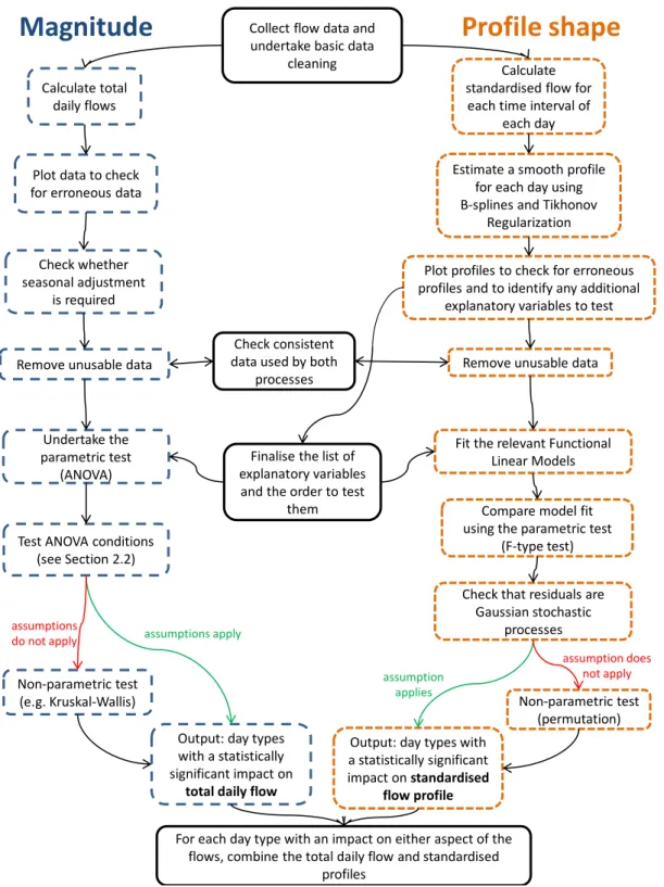
Figure 1 provides an overview of all of the stages which make up the proposed method. Total daily flows can be analysed using standard ANOVA methods, provided certain assumptions hold. The total daily flow needs to be normally distributed within each group and the population variance within each group should be equal. The observations should also be independent. Data should be tested for normality and for homogeneity of variances before ANOVA is undertaken. Where these assumptions do not hold, alternatives exist such as data transformation or non-parametric tests (for example the Kruskal-Wallis test used in Section 4). The independence assumption is required not just for ANOVA but also for non-parametric alternatives. To examine total daily flows, adjustments may need to be applied in order to remove seasonal and longer term trends, assuming a multiplicative relationship. This should provide a more stable basis for the day of the week testing. After applying a suitable test, a plot of the residuals can be examined to determine whether the independence assumption appears to be reasonable.
Collect flow data and undertake basic data
cleaning
Calculate total daily flows
Calculate standardised flow for
each time interval of each day
Output: day types with a statistically significant impact on
total daily flow
Fit the relevant Functional Linear Models
Check that residuals are Gaussian stochastic
processes
Non-parametric test (e.g. Kruskal-Wallis)
Estimate a smooth profile for each day using B-splines and Tikhonov
Regularization
Compare model fit using the parametric test
(F-type test) Undertake the
parametric test (ANOVA) Plot data to check for erroneous data
Test ANOVA conditions (see Section 2.2)
Remove unusable data Remove unusable data
Plot profiles to check for erroneous profiles and to identify any additional
explanatory variables to test
Non-parametric test (permutation)
For each day type with an impact on either aspect of the flows, combine the total daily flow and standardised
profiles
Output: day types with a statistically significant impact on standardised
flow profile Finalise the list of
explanatory variables and the order to test
them Check whether seasonal adjustment is required assumptions apply assumption applies assumptions do not apply
assumption does not apply
Magnitude
Profile shape
Check consistent data used by both
processes
Figure 1: Overview of methodology to clean, fit appropriate models and apply statistical significance tests to traffic flow data to produce representative flow profiles for each significantly different day type
3.1. Estimating daily flow profiles using B-splines
Although there are many ways in which time series data can be expressed, for the approach used in this paper each daily flow profile needs to be represented by a smooth curve. The success of the functional regression will, to a large extent, depend on the quality of this curve estimation process.
parameters vary from day to day (as in Watling et al. (2004, p45 onwards) in relation to travel times). In this research it is important to retain key features in the data such as the start and end times of peak periods and the gradient of the profile through the peak and therefore greater flexibility is required. A commonly used approach is to represent each function as a linear combination of functions, these component functions known as basis functions. Using a linear combination of basis functions is a flexible approach with computational advantages (Ramsay and Silverman, 2005).
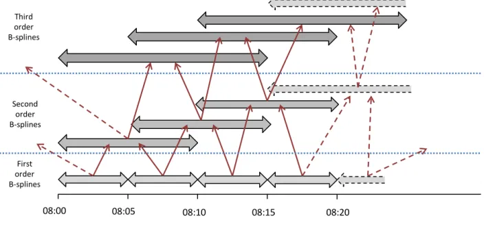
The basis function should be chosen so as to best represent the key features of the data. For example, a Fourier series basis would not be an obvious choice in this case as it is a periodic function. Whilst other bases could reasonably be used, for example a wavelet basis, in this paper B-splines will be used. B-splines are often used as de Boor (2001, p95) has shown that all polynomials of order p can be represented as linear combinations of B-splines of that order. This is particularly important given the distinctive M-shaped nature of daily flow profiles. B-splines are piecewise polynomials which are specifically designed so that they have continuous (p-1)th order derivatives (where p is the degree of the polynomial used), even where the pieces join. This means that cubic B-spline representations of the daily flow profiles would have continuous second order derivatives. Each B-spline is piecewise polynomial with compact support, i.e. it is non-zero on one small section of the estimation interval only Ramsay and Silverman (1997, p49). This is also an attractive property of B-splines, as demonstrated in
Figure 2, as the overlapping produces functional estimates which are better able to represent local features in the data than methods which consider the entire interval at once, for example Fourier or polynomial bases (Ramsay and Silverman, 1997, p48). Using B-splines, and cubic B-splines in particular, also makes the curve estimation process consistent with the method used on daily traffic flow profiles in Guardiola et al. (2014).
First order B-splines
Second order B-splines
Third order B-splines
08:00 08:05 08:10 08:15 08:20
Figure 2: B-spline coverage example
spans, which in Figure 2 are five minute intervals. In this paper, only uniform knot spacing with knots coinciding with data points has been considered. This is to ensure consistency across all functions estimated and because a roughness penalty will be included in the estimation process (see below). The process starts with the construction of a first order B-spline for each knot span as shown in equation (1):
(1)
where is the B-spline with knot k as the defining point (on the left hand side) and of order 1. is the time of day relating to the start of the kth subinterval. The first order B-splines, , are simply step functions taking the value 1 in [tk, tk+1] and 0 elsewhere.
The Cox-de Boor recursion relationship (de Boor, 2001, p90) shown in equation (2) can then be used to define B-splines of higher orders.
(2) where:
Once the B-splines have been generated, the coefficients in the linear relationship need to be estimated based on the standardised flows, , to produce suitable estimates of the daily flow profiles. Even though the daily flow profiles are estimated using cubic B-splines which guarantee continuous second order derivatives, they may still be “’rough’ or ‘wiggly’” (Green and Silverman, 1994, p4) if estimated using a least squares estimation process.. In order to find the optimal balance between capturing local features in the daily profiles and retaining excessive noise, a roughness penalty can be added within the least squares estimation process used to estimate the daily flow profiles from the count data (Ramsay and Silverman, 1997, Chapter 4). This is Tikhonov Regularization applied to functional data. The roughness penalty, denoted by , can take many forms in FDA, but the integrated squared second derivative is commonly used (Silverman, 1985, Green and Silverman, 1994, Ramsay and Silverman, 1997), resulting in the following formula for the penalized residual sum of squares to be minimised:
(3)
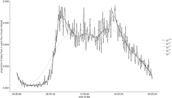
selected to use in the analysis. The suitability of the selected using the cross-validation method will be discussed further in section 4.2.2.
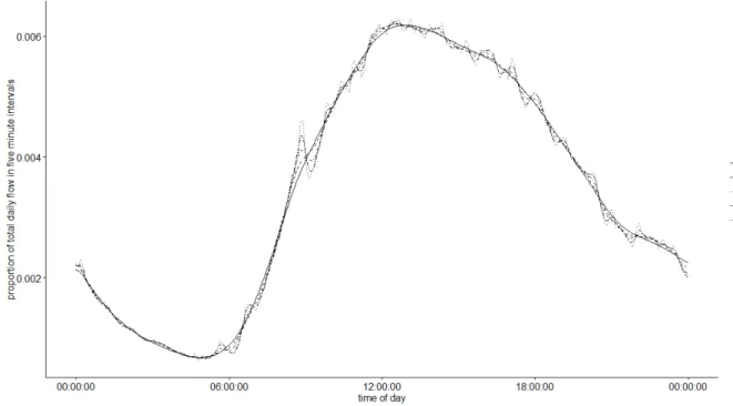
Figure 3: Estimated daily flow profiles for one day for a site in Greater Manchester with different roughness penalties applied
3.2. Analysing functional data
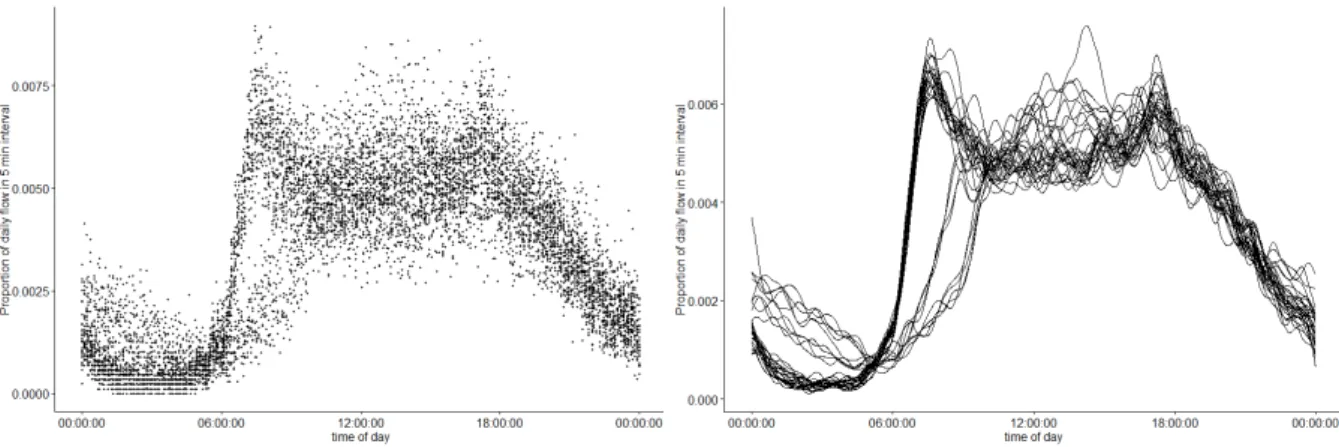
Whilst Figure 3 demonstrates the standardised flow profiles which could be estimated from flow data from one day (using different values of lambda), this process needs to be repeated for each day within the dataset. Figure 4 shows the (i.e. the fifteen minute aggregated flows) on the left hand side and the associated (the estimated flow profiles) on the right hand side, for one month of data from the case study site in Greater Manchester. The value of lambda used for every day was 10-6, as determined by a cross-validation procedure. Although the morning weekday flows follow a similar pattern, the heights of the peaks, between-peak and evening flows vary greatly. Figure 4 emphasises
that despite the use of a roughness penalty, the functions on the right hand side are ‘messy’ individual
observations which will require additional processes to analyse. Even from this one month of data, it
Figure 4: One month of standardised traffic flows represented by point data (left side) and by estimated functional observations (right side)
3.2.1. Functional linear models with functional responses
The relationships between day type identifiers, such as the day of the week, and daily flow profiles can be explored using an extension to linear modelling where the responses are functions, proposed by Ramsay and Silverman (1997). A Functional Linear Model with a functional response has the following structure:
Z t (4)
Or in alternative notation:
(5)
Here, is a vector of functional responses with respect to continuous time, t, which in this case
would be the daily flow profiles. Z is a design matrix consisting of entries , which are 1 if day is of type and 0 otherwise. is, therefore, a vector of functional coefficients. is a vector of functional residuals which represent the unexplained variability after the day type variables have been taken into account. These residuals are assumed to be statistically independent (Ramsay et al., 2009, p60).
to construct, but the need to be estimated by seeking to minimise the residuals (as is
known).
3.2.2. Fitting the model
In the current research the aim is not to estimate for all possible day types, but to identify the
most important day type variables to include in the model and then estimate the relevant coefficients. As testing all possible combinations of the dummy variables is not viable for larger problems, the standard forward stepwise regression process will be used. In practice this could begin with the structure currently used (for example just including a weekend/weekday split) and then test whether adding any other indicators would increase the explanatory power of the model.
Techniques for simultaneous variable selection and estimation, such as LASSO (Tibshirani, 1996), have been applied in functional analysis contexts (Matsui and Konishi, 2011, Lian, 2013, Mingotti et al., 2013). In the current application, however, a non-automated process has been used so that expert knowledge could be used to specify the hierarchy of variables to consider. In the example presented in Section 4 the separation of weekdays and weekend days will be considered first, then individual days of the week, and then seasons. The order of the hierarchy matters because each stage of testing is undertaken separately for each significantly different subset identified in the previous stage. In order to fit the models, a functional extension to the least squares approach will be used to estimate the day type coefficients, . As there is an area between the observed and predicted daily flow profiles, the term to be minimised can be expressed (Ramsay and Silverman, 1997, p141) as:
(6)
To be consistent with the least squares approach, F type tests comparing the fit of nested model specifications will be used to determine the most appropriate model to use. This is equivalent to
testing the null hypothesis that the ‘reduced’ model, including fewer predictor variables, is preferable
to the ‘full’ model which includes one or more additional predictor variables. Ramsay and Silverman (2005) suggest undertaking F-tests at each x-value, to produce point-wise test statistics for functional data. This would not, however, provide information about the statistical significance of the functional model, even if all of the point-wise tests are significant (Górecki and Smaga, 2015).
As an alternative to producing point-wise statistics, tests have been proposed to measure the overall significance of a functional model (see Górecki and Smaga (2015)). The F-type test proposed by Shen and Faraway (2004) for linear models with functional responses will be used as it is relatively easy to apply and Shen and Faraway (2004, p1256) assert that it “examines important rather than
trivial differences between models”. The test involves calculating a single value for each model comparison as follows:
Where RSS is the residual sum of squares, df is the degrees of freedom and the subscripts show whether the value refers to the reduced or the full model. The residual sum of squares is calculated by laying a fine grid over the profiles as an approximation for the area between the two curves.
The distribution of , the functional F distribution, can be estimated by the ordinary F distribution with degrees of freedom and , where is the degrees of freedom adjustment factor (Shen and Faraway, 2004, p1246). In practice, the method can be easily applied by laying a fine grid over the functions, as demonstrated in Yang et al. (2007). The degrees of freedom adjustment factor can then be estimated (Shen and Faraway, 2004, p1246) by:
After laying a fine grid over the functions, it is straightforward to compile E, the empirical covariance matrix based on the full model, using the covariances between flows at each time of the day corresponding to the fine grid. This F-type test assumes that the residuals are Gaussian stochastic processes. This assumption will be considered further in Section 4.2.2.
3.3. Combining the total daily flows and standardised flow profiles
The day types identified using the total daily flows and using the standardised flow profiles should then be considered alongside one another in order to observe systematic differences and consider the implications. The standardised flow profile for each day type should then be scaled up by the relevant total daily flow or flows for use as dynamical model inputs. This final stage is represented by the box at the bottom of Figure 1 which combines the outputs from the magnitude and profile shape processes.
4. EMPIRICAL STUDY
The methodology described in the previous section was applied to data from a loop detector on a key arterial route into Manchester. The road is a single lane urban road connecting Stockport (a large town approximately 6 miles south east of Manchester) to the city of Manchester. Two years of data (from 1/05/2013 to 30/04/2015) was used in the analysis. Data relating to public holidays was removed prior to the analysis as the profiles differed from non-public holiday days and yet they were not a homogenous group with sufficient sample size to include in the model. The B-spline estimation and the Functional Data Analysis were undertaken using the ‘fda’ package in R (Ramsay et al., 2014). The results will be presented, firstly for the analysis of the total daily flow data and then for the analysis of the daily profiles. Section 4.2 then includes a discussion of the smoothing parameters used, treatment of outliers and an analysis of the residuals from the same analysis.
4.1. Results
A non-parametric test was required to assess the impact of the day of the week on the total daily flow
as there is insufficient evidence to reject the null hypothesis in Levene’s test for the homogeneity of
variances (p=0.40), but the data is not Gaussian distributed (from visual inspection and Shapiro-Wilk test (p<0.001)). The day of the week had a statistically significant impact (Kruskal-Wallis test statistic 495, p<0.05) on total daily flow for this location, with two exceptions: flows on Thursdays and Fridays were not significantly different and neither were flows on Tuesdays and Wednesdays. As monthly adjustment factors have been applied, a formal test of seasonal differences in total daily flows has not been undertaken.
The shape of the daily flow profiles were considered next. To remove the magnitude effect (which was considered above), the flow profiles were transformed into the percentage of flows through the day relative to the total flow for that day. A smooth daily profile was then estimated for every day of data.
The results of the step-wise regression are presented in Figure 5. Each row represents a model formulation with the regression coefficients shown. Green arrows indicate statistically significant F-type test results ( ), i.e. where the full model is preferable to the reduced model.
Figure 5: Step-wise regression results for the site in Manchester
Figure 6: Average flow profiles for Saturdays and Sundays
There are many similarities between the average profiles for weekdays shown in Figure 7. Although the F-type tests have identified statistically significant differences between the profiles for each day of the week, this does not necessarily mean that all parts of the profiles are significantly different. To explore the differences in more detail, confidence intervals can be plotted around these functional coefficients. The confidence intervals can usually be calculated using the ‘fda’ package in R, but the case study dataset was too large to use this method, even using High Performance Computing, and therefore a suitable approximation was required.
Pointwise confidence intervals were estimated for the average standardised flow at five minute intervals throughout the day for each day of the week. The average flows for each day of the week at each time interval are a rough approximation for the functional coefficients from the FLM. Bootstrapping was used and therefore no distributional assumptions were made. The pointwise 95% confidence intervals for the average standardised flows on Thursdays and Fridays are shown in Figure 8. Although the intervals overlap for most of the day, there are times of the day where there is no overlap. The intervals are separate as flows increase before the morning peak, as they decrease after the evening peak (see inset) and at times between the peaks. The fact that the confidence intervals for Thursdays and Fridays do not always overlap is also a reflection of the relatively large amount of data available for this analysis as this has an effect on the interval widths. Other weekday comparisons showed different times of the day at which profiles differ.
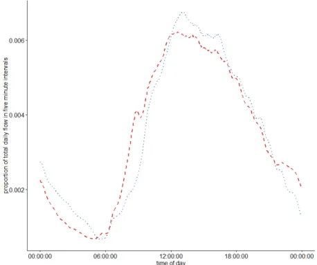
The day of the week may be expected to have an impact on daily flow profiles, but the method can also be used to explore less obvious impacts. Figure 9 shows the estimated seasonal coefficients when step-wise regression was undertaken on data from non-holiday Mondays only. In this case, winter and summer have a significant impact on flow profiles, but the profiles in spring and autumn were not statistically significantly different from one another ( ). The winter profile includes a smaller proportion of flows in the morning peak and a larger proportion in the middle of the day, perhaps indicating a higher proportion of non-commuting trips during the holiday season. The seasonal differences are far more pronounced during the morning peak and the inter-peak period than during the evening peak.
Figure 9: Standardised flow profiles by season for non-holiday Mondays
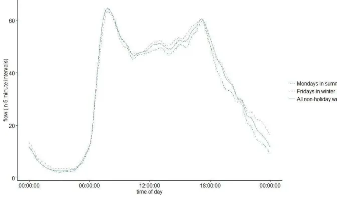
The total daily flows and the flow profiles estimated under the different day types should then be combined to produce a suitable input for within-day dynamical models. Figure 10 includes some examples of day types which may be considered for further investigation based on the full results from the analysis above. These have been constructed by combining the estimated total daily flow, using data from the relevant months and days of the week, and regression coefficient (for example ) for the relevant day type. In this example, the profiles suggest that if the link is close to capacity or a time of day dependent policy is being considered, modelling effects just based on average weekday conditions is unlikely to be sufficient.
Figure 10: Example flow profiles
4.2. Discussion
4.2.1. Considerations in applying the model
Figure 11: Saturday coefficients for lambda between 10-8 and 10-4
Another significant decision made in the analysis was to only exclude daily profiles where the data was known to be incorrect due to data collection issues. Other individual profiles which visually would appear to be outliers were included in the analysis. Note that the identification of individual outlier profiles is different from the exclusion of Bank Holidays which could be done a priori using dates alone and therefore is a well defined day type which is not suitable for inclusion in the analysis.
Keeping individual ‘outliers’ in the data ensured that the full range of flow profiles actually observed were included so as not to bias any analysis by only including those which were perceived to be near
some ‘expected’ profile. If the decision was made to exclude outliers, they could be identified using various methods including methods based on Principal Component Analysis (Chiou et al., 2014), influential observations (Shen and Xu, 2007) and the measurement of the ‘depth’ of a set of functions as used in Guardiola et al. (2014).
4.2.2. Analysis of residuals
Figure 12: Total daily flow residuals after seasonal adjustment, excluding December and early January data
The functional residuals arising from the Functional Linear Model also need to be considered. Each residual from the day of the week model can be calculated using:
t (9)
where is the vector of day type indicators relating to day i. These are residuals from the Functional Linear Model only and therefore only consider the smoothed functions and not the underlying point data. In this research the curve estimation process used is well established and therefore the residuals generated by moving from the point to the curve data do not require additional investigation.
Figure 13: The First Four Principal Components of the Residuals
The F-type test used in Section 4.1 relies on the assumption that the functional residuals are independent Gaussian stochastic processes (Shen and Faraway, 2004). Shen and Xu (2007) proposed visualising the Q-Q plot of studentized residuals against a Chi Squared distribution with degrees of freedom. The plot for the data analysed above is shown in Figure 14.
Clearly the plot is not a straight line as expected if the assumption holds. To test whether this was due to outliers in the data, the regression process was repeated after excluding influential outliers which
were identified using Cook’s Distance (Shen and Xu, 2007). The resulting Q-Q plot was not a straight line either. Further testing identified that the distribution of the studentized residuals had a higher kurtosis than the associated Chi Squared distribution. When the Gaussian assumption does not hold, permutation tests can be used to estimate the distribution of the test statistic rather than using the F distribution (Zhang, 2013). Good (1994) is a comprehensive text on permutation tests for point data, and other authors have applied these techniques to functional data (Muñoz Maldonado et al., 2002, Zhang, 2013, Corain et al., 2014). In a permutation test, the ‘labels’ connecting explanatory variables to observations are rearranged, and the test statistic is computed for this new, permuted dataset. This process is repeated until a large enough sample of all possible permutations has been collated. This sample provides information about the distribution of the test statistic under the null
hypothesis that the ‘labels’ do not provide any information about the observed value. The test statistic
computed using the correct labels is then compared to this distribution. Permutation tests provide a flexible way of testing hypotheses where distributional assumptions do not apply, but they are very computationally intensive in comparison to the F-type test.
A sample permutation test was undertaken for the final stage of the weekday analysis, namely the hypothesis that Tuesdays and Wednesdays have significantly different daily flow profiles. The Tuesday and Wednesday indicators were shuffled 5,000 times and the test statistic was computed for each permutation. This process had a running time of approximately 100 hours, but improvements could be made to speed up the process, for example by running sets of permutations in parallel. The 95th percentile of the distribution, i.e. the critical value, obtained was 1.82 which compares to the estimated critical value based on the F distribution above of 1.17. The value of the test statistic was 5.06 and therefore the outcome of the test is the same under either critical value. This may not always be the case, however, so permutation testing should always be considered if the Gaussian assumption is not satisfied.
5. CONCLUSIONS AND FUTURE WORK
In this paper we present a method for identifying day types, relating to the day of the week or time of year, with systematically different daily flow profiles. The method utilises Functional Data Analysis which is not often used in transportation research. This approach has advantages as it can retain the complexity of within day flow dynamics whilst having the conceptual simplicity of having one observation (in the form of a profile) to represent each day. We describe how data can be transformed into functional data and how linear models can be developed using the data. We also present a statistical method for identifying the preferred model formulation and thus the day type factors which have a statistically significant effect on flow profiles. The example using real-life traffic flow data identified that all seven days of the week had distinctive differences in the shape of the daily flow profile at this site. These differences included the timing and intensity of peak periods but also differences during the night, which is increasingly of interest.
varying congestion charges that themselves vary by day of the week or season; incentives to influence employers or shopping centres to adjust their opening times by day of the week or season; targeting public transport provision so that timetables are more responsive to the day of the week and seasonal needs of travellers.
The method in this paper could be built upon to analyse multiple sites. One approach could be to analyse sites independently and then develop a classification of sites based on the daily flow profile coefficients, or extract ‘global’ effects. Alternatively a more complex model could be developed to account for link correlations so that the relative attractiveness of routes under different scenarios could be considered. As well as considering flows, future work could also consider systematic differences in capacity, perhaps due to lighting (van Goeverden et al., 1998, Tenekeci et al., 2010) or/and weather effects (El Faouzi et al., 2010, Calvert and Snelder, 2013). Day-to-day dynamical models (for example from Watling and Cantarella (2013b)) could be extended to incorporate predictable differences, both in terms of input variables such as demand, but also by extending the transition functions between days to account for day type specific learning. The models including stochastic demand in Watling and Cantarella (2013b, Section 4) could also be extended so that the stochastic demand relates to functional data, i.e. randomly selected daily profiles as opposed to single values.
6. ACKNOWLEDGEMENTS
This research has been funded by the UK Engineering and Physical Sciences Research Council and Highways England through an Industrial CASE PhD Scholarship. The authors would also like to thank Transport for Greater Manchester for allowing them access to the data used in this research and the referees for their comments.
7. REFERENCES
Böcker, L., Dijst, M. & Prillwitz, J. (2012) Impact of Everyday Weather on Individual Daily Travel Behaviours in Perspective: A Literature Review. Transport Reviews, 33, 71-91.
Calvert, S. C. & Snelder, M. Influence of rain on motorway road capacity – a data-driven analysis. 16th International IEEE Annual Conference on Intelligent Transportation Systems (ITSC 2013), 2013 The Hague, The Netherlands. 1481-1486.
Chen, K. & Müller, H.-G. (2014) Modeling Conditional Distributions for Functional Responses, With Application to Traffic Monitoring via GPS-Enabled Mobile Phones. Technometrics, 56, 347-358.
Chiou, J.-M., Zhang, Y.-C., Chen, W.-H. & Chang, C.-W. (2014) A functional data approach to missing value imputation and outlier detection for traffic flow data. Transportmetrica B: Transport Dynamics, 2, 106-129.
Clark, S. & Watling, D. (2005) Modelling network travel time reliability under stochastic demand. Transportation Research Part B: Methodological, 39, 119-140.
Corain, L., Melas, V. B., Pepelyshev, A. & Salmaso, L. (2014) New insights on permutation approach for hypothesis testing on functional data. Advances in Data Analysis and Classification, 8, 339-356.
Du, J., Wong, S. C., Shu, C.-W. & Zhang, M. (2015) Reformulating the Hoogendoorn–Bovy predictive dynamic user-optimal model in continuum space with anisotropic condition. Transportation Research Part B: Methodological, 79, 189-217.
El Faouzi, N.-E., de Mouzon, O., Billot, R. & Sau, J. (2010) Assessing the changes in operating traffic stream conditions due to weather conditions. Advances in Transportation Studies, 21A, 33-48. Faraway, J. J. (1997) Regression Analysis for a Functional Response. Technometrics, 39, 254-261. Ferraty, F. & Vieu, P. (2003) Curves discrimination: a nonparametric functional approach.
Computational Statistics & Data Analysis, 44, 161-173.
Gao, H. O. & Niemeier, D. A. (2008) Using functional data analysis of diurnal ozone and NOx cycles to inform transportation emissions control. Transportation Research Part D: Transport and Environment, 13, 221-238.
Good, P. (1994) Permutation Tests: A Practical Guide to Resampling Methods for Testing Hypotheses, New York, Springer.
Górecki, T. & Smaga, Ł. (2015) A comparison of tests for the one-way ANOVA problem for functional data. Computational Statistics.
Green, P. J. & Silverman, B. W. (1994) Nonparametric Regression and Generalized Linear Models: A Roughness Penalty Approach, London, Chapman and Hill.
Guardiola, I. G., Leon, T. & Mallor, F. (2014) A functional approach to monitor and recognize patterns of daily traffic profiles. Transportation Research Part B: Methodological, 65, 119-136.
Guo, F., Li, Q. & Rakha, H. (2012) Multistate Travel Time Reliability Models with Skewed Component Distributions. Transportation Research Record: Journal of the Transportation Research Board, 2315, 47-53.
Guo, R.-Y., Yang, H., Huang, H.-J. & Tan, Z. (2015) Link-based day-to-day network traffic dynamics and equilibria. Transportation Research Part B: Methodological, 71, 248-260.
Habib, K. M. N., Day, N. & Miller, E. J. (2009) An investigation of commuting trip timing and mode choice in the Greater Toronto Area: Application of a joint discrete-continuous model. Transportation Research Part A: Policy and Practice, 43, 639-653.
Habib, K. M. N. & Miller, E. J. (2008) Modelling daily activity program generation considering within-day and day-to-day dynamics in activity-travel behaviour. Transportation, 35, 467-484.
Han, K., Friesz, T. L., Szeto, W. Y. & Liu, H. (2015) Elastic demand dynamic network user equilibrium: Formulation, existence and computation. Transportation Research Part B: Methodological, 81, 183-209.
Hanson, S. & Huff, J. O. (1988) Systematic variability in repetitious travel. Transportation, 15, 111-135.
Hazelton, M. L. & Parry, K. (2015) Statistical methods for comparison of day-to-day traffic models. Transportation Research Part B: Methodological.
Järv, O., Ahas, R. & Witlox, F. (2014) Understanding monthly variability in human activity spaces: A twelve-month study using mobile phone call detail records. Transportation Research Part C: Emerging Technologies, 38, 122-135.
Jiang, X. & Adeli, H. (2005) Dynamic Wavelet Neural Network Model for Traffic Flow Forecasting. Journal of Transportation Engineering, 131, 771-779.
Kitamura, R. & Van Der Hoorn, T. (1987) Regularity and irreversibility of weekly travel behavior. Transportation, 14, 227-251.
Kumar, A. & Peeta, S. (2015) A day-to-day dynamical model for the evolution of path flows under disequilibrium of traffic networks with fixed demand. Transportation Research Part B: Methodological, 80, 235-256.
Lam, W. H. K., Shao, H. & Sumalee, A. (2008) Modeling impacts of adverse weather conditions on a road network with uncertainties in demand and supply. Transportation Research Part B: Methodological, 42, 890-910.
Lee, K. L., Meyer, R. J. & Bradlow, E. T. (2009) Analyzing risk response dynamics on the web: the case of Hurricane Katrina. Risk Anal, 29, 1779-92.
Li, L., Su, X., Zhang, Y., Lin, Y. & Li, Z. (2015) Trend Modeling for Traffic Time Series Analysis: An Integrated Study. IEEE Transactions on Intelligent Transportation Systems, 16, 3430-3439.
Lian, H. (2013) Shrinkage estimation and selection for multiple functional regression. Statistica Sinica.
Lo, H. K. & Tung, Y.-K. (2003) Network with degradable links: capacity analysis and design. Transportation Research Part B: Methodological, 37, 345-363.
Long, J., Szeto, W. Y., Gao, Z., Huang, H.-J. & Shi, Q. (2016) The nonlinear equation system approach to solving dynamic user optimal simultaneous route and departure time choice problems. Transportation Research Part B: Methodological, 83, 179-206.
Matsui, H. & Konishi, S. (2011) Variable selection for functional regression models via the L1
regularization. Computational Statistics & Data Analysis, 55, 3304-3310. May, A. D. (1990) Traffic flow fundamentals, Englewood Cliffs, Prentice Hall.
Mingotti, N., Lillo, R. E. & Romo, J. (2013) Lasso Variable Selection in Functional Regression. Working papers [Online]. Available:
http://orff.uc3m.es/bitstream/handle/10016/16959/ws131413.pdf?sequence=1.
Muñoz Maldonado, Y., Staniswalis, J. G., Irwin, L. N. & Byers, D. (2002) A similarity analysis of curves. The Canadian Journal of Statistics, 30, 373-381.
Nakayama, S. & Watling, D. (2014) Consistent formulation of network equilibrium with stochastic flows. Transportation Research Part B: Methodological, 66, 50-69.
Nerini, D. & Ghattas, B. (2007) Classifying densities using functional regression trees: Applications in oceanology. Computational Statistics & Data Analysis, 51, 4984-4993.
Ngoduy, D., Hoang, N. H., Vu, H. L. & Watling, D. (2016) Optimal queue placement in dynamic system optimum solutions for single origin-destination traffic networks. Transportation Research Part B: Methodological, In Press.
Noland, R. B. & Small, K. A. (1995) Travel-time uncertainty, departure time choice, and the cost of the morning commute. Irvine: Institute of Transportation Studies, University of California. Ozbay, K., Yang, H., Morgul, E. F., Mudigonda, S. & Bartin, B. Big Data and the Calibration and
Validation of Traffic Simulation Models. Looking Back and Looking Ahead: Celebrating 50 Years of Traffic Flow Theory, 2014 Washington D.C.: Transportation Research Board, 92-122.
Pu, W. (2011) Analytic Relationships Between Travel Time Reliability Measures. Transportation Research Record: Journal of the Transportation Research Board, 2254, 122-130.
Ramsay, J. O., Hooker, G. & Graves, S. (2009) Functional Data Analysis with R and MATLAB, New York, Springer.
Ramsay, J. O. & Silverman, B. W. (1997) Functional Data Analysis, New York, Springer. Ramsay, J. O. & Silverman, B. W. (2005) Functional Data Analysis, New York, Springer.
Ramsay, J. O., Wickham, H., Graves, S. & Hooker, G. (2014) Package ‘fda’ [Online]. The Comprehensive R Archive Network (CRAN). Available: http://cran.r-project.org/web/packages/fda/fda.pdf [Accessed: 17th December 2014].
Schlich, R. & Axhausen, K. W. (2003) Habitual travel behaviour: Evidence from a six-week travel diary. Transportation, 30, 13-36.
Shao, H., Lam, W. H. K. & Tam, M. L. (2006) A reliability-based stochastic traffic assignment model for network with multiple user classes under uncertainty in demand. Networks & Spatial Economics, 6, 173-204.
Shen, Q. & Faraway, J. (2004) An F Test for Linear Models with Functional Responses. Statistica Sinica, 14, 1239-1257.
Shen, Q. & Xu, H. (2007) Diagnostics for Linear Models With Functional Responses. Technometrics, 49, 26-33.
Silverman, B. W. (1985) Some Aspects of the Spline Smoothing Approach to Non-Parametric Regression Curve Fitting. Journal of the Royal Statistical Society: Series B (Methodological), 47, 1-52.
Siu, B. W. Y. & Lo, H. K. (2008) Doubly uncertain transportation network: Degradable capacity and stochastic demand. European Journal of Operational Research, 191, 166-181.
Stathopoulos, A. & Karlaftis, M. (2001) Temporal and Spatial Variations of Real-Time Traffic Data in Urban Areas. Transportation Research Record: Journal of the Transportation Research Board, 1768, 135-140.
Sumalee, A., Uchida, K. & Lam, W. H. K. (2011a) Stochastic multi-modal transport network under demand uncertainties and adverse weather condition. Transportation Research Part C: Emerging Technologies, 19, 338-350.
Sumalee, A., Watling, D. & Nakayama, S. (2006) Reliable Network Design Problem: Case with Uncertain Demand and Total Travel Time Reliability. Transportation Research Record: Journal of the Transportation Research Board, 1964, 81-90.
Sumalee, A., Zhong, R. X., Pan, T. L. & Szeto, W. Y. (2011b) Stochastic cell transmission model (SCTM): A stochastic dynamic traffic model for traffic state surveillance and assignment. Transportation Research Part B: Methodological, 45, 507-533.
Tang, J., Wang, Y., Wang, H., Zhang, S. & Liu, F. (2014) Dynamic analysis of traffic time series at different temporal scales: A complex networks approach. Physica A: Statistical Mechanics and its Applications, 405, 303-315.
Tenekeci, G., Montgomery, F. & Wainaina, S. (2010) Roundabout capacity in adverse weather and light conditions. Proceedings of the ICE - Transport, 163, 29-39.
Tibshirani, R. (1996) Regression Shrinkage and Selection via the Lasso. Journal of the Royal Statistical Society: Series B (Methodological), 58, 267-288.
Transport for London (2013) Olympic Legacy Monitoring: Personal Travel Behaviour during the Games Available: content.tfl.gov.uk/olympic-legacy-personal-travel-report.pdf [Accessed: 29th July 2016].
van Goeverden, C. D., Botma, H. & Bovy, P. H. L. (1998) Determining Impact of Road Lighting on Motorway Capacity. Transportation Research Record: Journal of the Transportation Research Board, 1646, 1-8.
Vlahogianni, E. I., Golias, J. C. & Karlaftis, M. G. (2004) Short term traffic forecasting: Overview of objectives and methods. Transport Reviews, 24, 533-557.
Vlahogianni, E. I., Karlaftis, M. G. & Golias, J. C. (2014) Short-term traffic forecasting: Where we
are and where we’re going. Transportation Research Part C: Emerging Technologies, 43, 3-19.
Wang, D. Z. W. & Du, B. (2016) Continuum modelling of spatial and dynamic equilibrium in a travel corridor with heterogeneous commuters—A partial differential complementarity system approach. Transportation Research Part B: Methodological, 85, 1-18.
Watling, D. (2002) A Second Order Stochastic Network Equilibrium Model, I: Theoretical Foundation. Transportation Science, 36, 149-166.
Watling, D., Sumalee, A., Connors, R. & Balijepalli, C. (2004) Advancing methods for evaluating network reliability: A Department for Transport "New Horizons" Project Final Report. Available:
http://webarchive.nationalarchives.gov.uk/20070306100043/http:/www.dft.gov.uk/pgr/econo mics/rdg/jtv/amenr/advancingmethodsforevaluatin3080 [Accessed: 14th May 2014].
Watling, D. P. & Cantarella, G. E. (2013a) Model Representation & Decision-Making in an Ever-Changing World: The Role of Stochastic Process Models of Transportation Systems. Networks and Spatial Economics.
Watling, D. P. & Cantarella, G. E. (2013b) Modelling sources of variation in transportation systems: theoretical foundations of day-to-day dynamic models. Transportmetrica B: Transport Dynamics, 1, 3-32.
Weijermars, W. & van Berkum, E. Analyzing highway flow patterns using cluster analysis. 8th International IEEE Conference on Intelligent Transportation Systems, 2005 Vienna, Austria. 831-836.
Weijermars, W. A. M. & van Berkum, E. C. (2004) Daily flow profiles of urban traffic. In: BREBBIA, C. A. & WADHWA, L. C. (eds.) Urban Transport X. Urban Transport and the Environment in the 21st Century. Dresden, Germany: WIT Press.
Xiao, F., Yang, H. & Ye, H. (2016) Physics of day-to-day network flow dynamics. Transportation Research Part B: Methodological, 86, 86-103.
Yang, X., Shen, Q., Xu, H. & Shoptaw, S. (2007) Functional regression analysis using an F test for longitudinal data with large numbers of repeated measures. Stat Med, 26, 1552-66.
Yazici, M., Kamga, C. & Mouskos, K. (2012) Analysis of Travel Time Reliability in New York City Based on Day-of-Week and Time-of-Day Periods. Transportation Research Record: Journal of the Transportation Research Board, 2308, 83-95.
Zhang, J.-T. (2013) Analysis of Variance for Functional Data. Boca Raton, Florida: CRC Press. Zhang, W., Mediria, A. & Rakha, H. (2007) Statistical analysis of spatiotemporal link and path flow