Time Variation in the Dynamics of Worker Flows : Evidence from the US and Canada

S

TRATHCLYDE

D

ISCUSSION

P

APERS IN

E

CONOMICS

D

EPARTMENT OF

E

CONOMICS

U

NIVERSITY OF

S

TRATHCLYDE

G

LASGOW

TIME VARIATION IN THE DYNAMICS OF WORKER FLOWS:

EVIDENCE FROM THE US AND CANADA

B

Y

MICHELE CAMPOLIETI, DEBORAH GEFANG AND

GARY KOOP

Time Variation in the Dynamics of Worker

Flows: Evidence from the US and Canada

Michele Campolieti

Department of Management, University of Toronto Scarborough

Centre for Industrial Relations, University of Toronto

Deborah Gefang

Department of Economics, Lancaster University

Gary Koop

Department of Economics, University of Strathclyde

September 24, 2011

ABSTRACT

VAR methods have been used to model the inter-relationships between

in-‡ows and outin-‡ows into unemployment and vacancies using tools such as impulse

response analysis. In order to investigate whether such impulse responses change

over the course of the business cycle or or over time, this paper uses TVP-VARs

for US and Canadian data. For the US, we …nd interesting di¤erences between

the most recent recession and earlier recessions and expansions. In particular,

we …nd the immediate e¤ect of a negative shock on both in‡ow and out‡ow

haz-ards to be larger in 2008 than in earlier times. Furthermore, the e¤ect of this

shock takes longer to decay. For Canada, we …nd less evidence of time-variation

in impulse responses.

JEL Classi…cation: J64; J63; C32.

Keywords: unemployment hazards, labor market dynamics, time-varying

1

Introduction

Changes in unemployment rates depend on both ‡ows into and out of

unem-ployment. Understanding how unemployment is a¤ected by both these ‡ows

has a attracted a great deal of attention in the literature. Since the seminal

work of Darby, Haltiwanger and Plant (1986), many studies have used

descrip-tive measures to investigate the ins and outs of unemployment (e.g. Hall, 2005,

Shimer, 2007, Elsby et al, 2009, Fujita and Ramey, 2006 and 2009 and

Campoli-eti, 2011, among many others). However, while these descriptive methods can

be helpful in characterizing the ‡ows into and out of unemployment as well as

changes in unemployment rates, they do not take into account dynamics so they

miss some aspects of the adjustment process in the labor market. Arguing that

descriptive measures may not be useful in disentangling shocks generated out

of the labor market, such as productivity shocks, from those generated within

the job search/matching system, Fujita (2011) uses VAR models to explore the

interrelationships between the ins and outs of unemployment and vacancy rates

in the US. He identi…es the structural VAR structure using the sign restriction

approach of Uhlig (2005). In particular, he identi…es a negative aggregate shock

as one which causes changes to unemployment to be negative forkquarters and

does not immediately raise vacancies. This is the framework on which we build

in the present paper.

The analysis of Fujita (2011) is conducted using a VAR with constant

co-e¢ cients and, thus, impulse responses which are also constant. This can be

potentially misleading if the mechanisms underlying the job search/matching

process are varying over time. Results of many studies (e.g. Hall 2005, Shimer

2007, Elsby et al, 2009) suggest that the dynamics of the ins and outs of

un-employment can be closely related to the ‡uctuations of business cycles. In the

1999 and Skalin and Teräsvirta, 2002) …nd considerable evidence of

nonlineari-ties in unemployment. To take account of these possible nonlinear e¤ects, this

paper extends Fujita (2011) by using a time-varying parameter (TVP) VAR.

We adopt the TVP-VAR of Primiceri (2005) which additionally allows for

mul-tivariate stochastic volatility and is popular in the empirical macroeconomics

literature. This framework is attractive since it allows both the VAR coe¢ cients

and the error covariance matrix to vary over time in a ‡exible and unrestricted

fashion.

We estimate VARs and TVP-VARs using three series: the in‡ow hazard

(job separation rate); the out‡ow hazard (job …nding rate); and, vacancies. We

use both Canadian and US data. Our empirical results provide support for the

TVP-VAR with multivariate stochastic volatility. This support is particularly

strong for the US data. We also …nd support for the inequality restrictions

we use to identify the impulse responses. These lead to uniformly sensible

responses to a shock for all the series we consider for both the US and Canada.

In particular, we …nd that the in‡ow hazard (separation rate) increases quickly

after a shock before declining slowly. In contrast, the out‡ow hazard (job …nding

rate) and vacancies decrease after a shock before increasing in a hump shaped

pattern. This general pattern holds for both the US and Canada. The only slight

di¤erence between the countries is that the impulse responses for Canada tend

to oscillate a bit before decaying in some cases. We do not …nd much evidence

of time variation in impulse responses using Canadian data. However, we …nd

some interesting time variation in the US data. While the impulse responses for

most of the time periods we consider are similar, the impulse responses for the

in‡ow and out‡ow hazard in the US Great Recession di¤er from earlier periods.

In particular, the in‡ow hazard tends to respond more strongly to a shock and

strongly initially and takes longer to decay and is still quite large at the end

of the time horizon we consider. These …ndings tend to be consistent with the

observations made by Elsby et al (2010a) on the US labor market during the

Great Recession.

2

Econometric Methods

VAR methods have enjoyed wide popularity in empirical macroeconomics since

the pioneering work of Sims (1980). VARs are atheoretical models which

al-low the researcher to investigate the relationships between time series variables

without imposing any economic theory. Structural identifying restrictions are

placed on VARs in order to give an economic interpretation to impulse responses

and other features of interest. Traditionally, these identifying restrictions have

been equality restrictions and, in some cases, have been criticized for being

overly strong. Uhlig (2005) proposes using weaker sets of inequality restrictions

in order to identify impulse responses. This attempt to impose the minimum

amount of economic theory used, and let the data speak, is in the spirit of the

atheoretical VAR literature. These considerations presumably motivated Fujita

(2011), who used a VAR involving in‡ow and out‡ow hazards and vacancy rates

along with a sign restriction approach.1 This approach required the minimal

as-sumptions that a negative shock cannot immediately raise vacancies and cannot

cause the unemployment rate to fall fork quarters.

Our econometric methods also begin with VARs with impulse responses

be-ing identi…ed through similar sign restrictions. However, we also use TVP-VARs

which allow for VAR coe¢ cients to change over time. In empirical

macroeco-nomics, there is a plethora of evidence of structural breaks and other kinds of

1_{Fujita (2011) also considers an expanded VAR, which includes additional shocks and}

parameter change (see, among many others, Stock and Watson, 1996) and this

has led to a large number of papers which use TVP-VARs (see, among many

others Cogley and Sargent, 2001, 2005, Cogley et al, 2005, Primiceri 2005, and

D’Agostino et al, 2009 and Koop et al, 2009). It is also worth noting that most of

these TVP-VARs paper allow for multivariate stochastic volatility which seems

to be empirically important in many macroeconomic applications. One purpose

of the present paper is to see whether TVP-VARs with multivariate stochastic

volatility will prove equally useful in applications in labor economics.

In this section, we brie‡y outline the structure of TVP-VARs and describe

how we implement the sign restriction approach to impulse response analysis.

The Technical Appendix provides additional details. Our TVP-VAR setup

fol-lows Primiceri (2005) and the sign restriction approach is implemented as in

Uhlig (2005) and the reader is referred to these papers for additional motivation

and explanation.

The basic VAR used by Fujita (2011) can be written as

yt=Zt +"t (1)

whereytis ann 1vector of observations on the dependent variables,Ztis an

n mmatrix of containing a vector of intercepts and lagged dependent variables

and"tare independentN(0; H)fort= 1;2; :::; T. The TVP-VAR extends this

as

yt=Zt t+"t (2)

where

t= t 1+ t: (3)

and _tare independentN(0; Q). Notice that this takes the form of a state space

vector of unobserved states. This is a popular speci…cation which allows for the

coe¢ cients to vary over time. It has the advantage that standard statistical

methods for state space models exist. In our empirical work, we refer to this as

the homoskedastic VAR, to distinguish it from the heteroskedastic

TVP-VAR which assumes"t are independent N(0; Ht). Following Primiceri (2005),

we use a triangular decomposition to modelHt:

Ht=At1 t 0 t(At1)

0

; (4)

where t is a diagonal matrix with diagonal elements j;tforj= 1;2; :::; nand

Atis a lower triangular matrix with ones on the diagonal. That is, it takes the

form:

At=

0 B B B B B B B B B B @

1 0 ::: : 0

a21;t 1 ::: : :

: : ::: : : : : ::: 1 0

an1;t : ::: an(n 1);t 1

1 C C C C C C C C C C A

Let t= ( 1;t; 2;t; :::; n;t)0 andat= (a21;t; a31;t; a32;t; :::; an(n 1);t)0. These

are allowed to evolve according to the following state equations:

log( t) =log( t 1) +ut; (5)

and

at=at 1+vt; (6)

whereut i:i:d:N(0; W), vt i:i:d:N(0; C), andutandvtare independent to

each other with all the leads and lags. As discussed in Primiceri (2005), this

speci…cation is a ‡exible one, allowing both error variances and covariances to

Our empirical work considers VARs, homoskedastic TVP-VARs and

het-eroskedastic TVP-VARs. We use the Bayesian information criterion (BIC) to

compare these models. This can be interpreted as an asymptotic approximation

to the log of the marginal likelihood (the conventional Bayesian model

compar-ison metric). Note that BIC does not involve the prior, which is potentially

an advantage in high-dimensional models such as VARs and TVP-VARs where

marginal likelihoods can be sensitive to prior choice. Following Carlin and Louis

(2000, Section 6), we calculate the BIC using the posterior expectation of the

log-likelihood.

Additional technical details, including discussion of posterior simulation and

the priors used in our Bayesian estimation procedure, are given in the Technical

Appendix. The reader is referred to Koop and Korobilis (2009) for complete

details Bayesian estimation of VARs and TVP-VARs.

The Technical Appendix also gives details of how the sign-restricted impulse

responses are calculated. We use the same methods as Uhlig (2005) and Fujita

(2011). These require the speci…cation of restrictions and we use the same

restrictions as in Fujita (2011) which identify an aggregate shock using the

following restrictions:

1. A negative aggregate shock will causes changes in unemployment to be

non-negative forkquarters.

2. A negative aggregate shock will not raise vacancies in the impact quarter.

In line with Fujita (2011), in this paper we setk= 2. In the online empirical

appendix, we also present results for k = 1;3;4 and …nd results to be fairly

robust to choice ofk.

Note that the …rst restriction relates to the unemployment rate. Following

(uet) by the steady-state unemployment rate:

uet

st

ft+st

wherestis the in‡ow hazard andftis the out‡ow hazard.

We present impulse responses for the three variables in yt (i.e. the in‡ow

and out‡ow hazards and the vacancy rate) plus the unemployment rate. With

regards to the latter we proceed as follows. After a shock at time t, if the

responses of the in‡ow hazard and out‡ow hazard at time t+ 1 are irfs;t+1

andirff;t+1, respectively, the impulse response of unemployment at timet+ 1

(irfue;t+1) can be approximated by the following equation:

irfue;t+1

st+irfs;t+1

ft+st+irfs;t+1+irff;t+1

uet

Similarly, the impulse responses of unemployment for future horizonsthr, which

is longer than1, can be approximated by:

irfue;t+thr

st+Ptiihr=1irfs;t+ii

ft+st+Ptiihr=1(irfs;t+ii+irff;t+ii)

st+Ptiihr=11irfs;t+ii

ft+st+Piithr=11(irfs;t+ii+irff;t+ii)

In our empirical work, we also present a variance decomposition arising from

the sign-restricted impulse response approach. De…ned as in Fujita (2011), this

measures the proportion of the forecast error variance at di¤erent horizons which

can be attributed to the identi…ed aggregate shock.

3

Empirical Results

We divide our empirical results section into three sub-sections. The …rst

de-scribes the data while the second discusses modelling choices and volatility

decom-positions.

3.1

Data

We use quarterly data from the US and Canada. The US data runs

1951Q1-2009Q4, while the Canadian data spans 1981Q1 through 2003Q2. The shortness

of the Canadian data is due to the decision of Statistics Canada to terminate

the help wanted index in April, 2003.

The US data were obtained from Elsby et al (2010a) and include the in‡ow

and out‡ow hazard series, which were computed using data from the Current

Population Survey (CPS), as well as a help wanted index. The US help wanted

index is collected by the Conference Board and is based on help wanted ads in

51 prominent newspapers in the US. The Canadian in‡ow and out‡ow hazard

series were originally computed in Campolieti (2011) using the public release

…les of the Labour Force Survey (LFS), which is collected by Statistics Canada

and is comparable to the US CPS. The help wanted index is obtained from

Statistics Canada’s CANSIM database.2 The Canadian help wanted index is

based on the number of job ads in newspapers and is comparable to the US

help wanted index we use.3 _{The in‡ow and out‡ow hazard rates for both the}

US and Canada are based on the framework introduced by Shimer (2007) with

the re…nements in Elsby et al (2009). These hazard rates measure the ‡ows

into unemployment and out of unemployment.4 _{Details on the computation of}

the in‡ow hazards can be found in Elsby et al (2009), Elsby et al (2010a) and

Campolieti (2011).

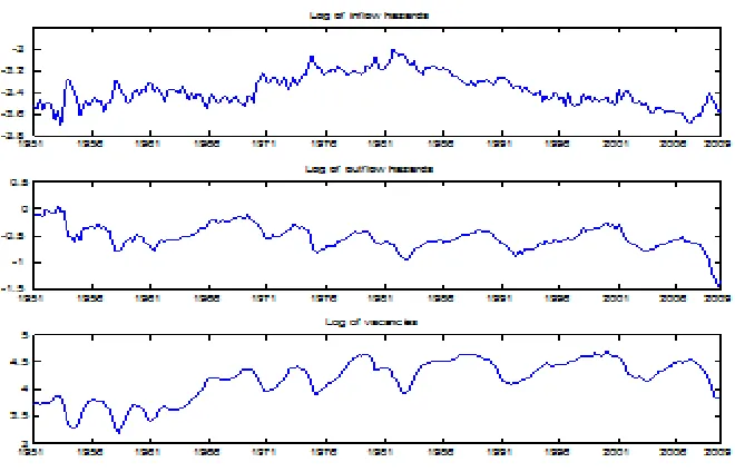
Figures 1 and 2 plot the raw data for the US and Canada, respectively.

2_{This help wanted index was introduced during the …rst quarter of 1981.}

3_{There was also an earlier help wanted index that was available from 1962 to 1988. This}

index was proportional to the space occupied by job o¤ers in Canada’s major newspapers, but is was not a robust a measure because it was sensitive to changes in fonts and column widths as well as paper size in the newspaper industry.

It can be seen that there is some evidence of low-frequency trends in the data.

Fujita (2011) argues that theoretical search/matching models are not associated

with low-frequency trends and, accordingly, takes out such low frequency trends.

Following Fujita (2011), we detrend all our series using deterministic quadratic

trends.

Figure 2. Canadian data

3.2

Model Comparison

BIC chooses VAR models with lag length 2 for the US and Canada and we adopt

this choice for all of our VARs and TVP-VARs. With regards to the degree of

time-variation in VAR coe¢ cients and error variances, Table 1 presents BICs for

three models. For notational convenience, we use ’Homo TVP-VAR’to denote

TVP-VAR models with constant error covariance matrix, and ’Hete TVP-VAR’

to denote TVP-VAR models with time varying error covariance matrix. Table 1

indicates moderately strong support for time-variation in both VAR coe¢ cients

and the error covariance matrix. That is, for both countries the Homo

VAR has a substantially lower BIC than the VAR and the heteroskedastic

TVP-VAR in turn has a substantially lower BIC than the TVP-TVP-VAR. Accordingly, in

TVP-VAR. However, a complete set of results for all models is available in the online

appendix.

Table 1: BIC for Various Models

Canada US

VAR 6.6504 7.5446

Homo TVP-VAR -0.4346 -1.6442

Hete TVP-VAR -8.1602 -9.0031

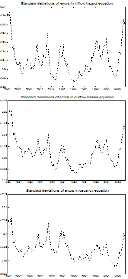
To shed light on the importance of allowing for stochastic volatility, Figures

2 and 3 plot the posterior means of the standard deviations of the errors in

the three equations of the TVP-VAR for the US and Canada, respectively. For

both countries, there is evidence of time variation, but the patterns are quite

di¤erent. For Canada, the time variation reveals itself largely through a spike

around 1997. For the longer US series, we see more peaks and troughs in

the volatilities. Furthermore, a careful examination of the scale of the Y-axis

indicates that it is only for the in‡ow hazard that substantial time variation in

the error variance occurs. For Canada, Campolieti (2011) notes that there is a

spike in the in‡ow hazard around 1997 and examines some other data sources for

similar patterns. Campolieti (2011) concludes that the spike in the in‡ow hazard

was likely related to changes in the LFS that occurred around this time, since the

spike is not present in other data. More speci…cally, there was increased use of

CATI interviews, changes in the survey questionnaire that added new variables

and, most importantly, a change in the wording of the temporary layo¤ question

that was phased in between September 1996 and January 1997 (Sunter et al,

1997) that would classify more individuals as unemployed. Campolieti (2011)

also observes an increase in the Canadian out‡ow hazard around 1997. This

increase in unemployment out‡ows is equivalent to a decrease in unemployment

Campolieti (2011) notes the reasons for this increase in the out‡ow rate from

unemployment are unclear.

3.3

Impulse Response Functions and Variance

Decompo-sitions

For each country, we calculate impulse responses and variance decompositions

for various time periods. For the US, dates near business cycle troughs of

1982Q4, 1992Q3 and 2003Q2 are chosen as well dates near peaks of 1989Q2,

2000Q4. In addition, we use 2008Q2 to examine the e¤ect of the recent crises.

For Canada, troughs are 1982Q4, 1992Q4 and 2002Q1.5 Peaks are around

1989Q3 and 2000Q2. We also include 2003Q1 as the last observation in the

Canadian sample.

3.3.1 Variance Decompositions

Before presenting impulse responses, we provide information that the sign

re-strictions used to calculate them are reasonable ones. Tables 2 and 3 present a

summary of the variance decompositions for the US and Canada, respectively

(…gures containing a full set of variance decompositions, including credible

inter-vals, are available in the online appendix). The variance decompositions were

calculated up to a horizon of 20 quarters. The tables present the average of

the point estimate over all horizons. Tables 2 and 3 indicate that the aggregate

shock we have identi…ed accounts for an appreciable amount of the variability in

all three of our variables. For the US, it account for roughly 40-45% of the

vari-ability in all three series. For Canada, comparable numbers are about 30-33%.

These are similar to the …gures presented in Fujita (2011) for his benchmark

VAR.

Table 2: Average Variance Decomposition Rates for Hetero TVP-VAR, US

Time Q4 1982 Q2 1989 Q3 1992 Q4 2000 Q2 2003 Q2 2008

In‡ow Hazard 0.3888 0.3907 0.3914 0.4062 0.3950 0.4121

Out‡ow Hazard 0.4420 0.4429 0.4422 0.4394 0.4310 0.4376

Vacancies 0.4444 0.4393 0.4393 0.4414 0.4349 0.4422

Table 3: Average Variance Decomposition Rates for Hetero TVP-VAR, Canada

Time Q3 1989 Q4 1992 Q2 2000 Q1 2002 Q1 2003

In‡ow Hazard 0.3328 0.3206 0.3262 0.3281 0.3326

Out‡ow Hazard 0.3231 0.3102 0.3137 0.3164 0.3223

Vacancies 0.3289 0.3167 0.3234 0.3249 0.3249

3.3.2 Impulse Response Functions

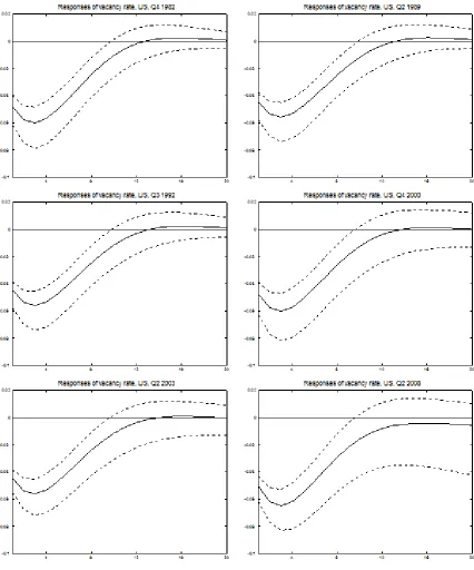
Figures 5 through 8 present impulse responses for the US data with Figures 9

through 12 repeating the analysis for the Canadian data. All of these …gures are

responses to the aggregate shock identi…ed using the sign restrictions. The four

…gures for each country are responses of four variables (in‡ow hazard, out‡ow

hazard, unemployment rate and vacancy rate) to this shock at the time periods

speci…ed above. In all these …gures the solid line is the posterior median and

the dashed lines are the 16th and 84th percentiles of the posteriors. We present

results only for the heteroskedastic TVP-VAR, but occasionally refer to results

for other models. These latter results are available in the online appendix.

US Results

The response of the in‡ow hazard to the aggregate shock dies o¤ steadily

and fairly quickly (in about 8 quarters). In contrast, the out‡ow hazard,

unem-ployment and vacancy variables exhibit hump-shaped patterns. These impulse

responses tend to be near zero after about 3 or 4 years. These general

homoskedastic TVP-VAR.

The sign of the response for all the series we consider are unambiguous

(i.e. they never ‡ip from being positive at some horizons and negative at

oth-ers), which provides support for the restrictions we use in the data. In other

words, despite using weak restrictions we observe some features of the

adjust-ment process in the US labor market quite clearly. The in‡ow hazard

(sep-aration rate) reaches its peak quickly and then declines slowly. The out‡ow

hazard (job …nding rate) and vacancies take a few quarters to reach the trough

before starting to fade. The patterns in these series are like those in Fujita

(2011). Moreover, they also support the conclusions in Elsby et al (2009) and

Fujita and Ramey (2009) that unemployment dynamics in the US are driven by

‡uctuations in both the in‡ow and out‡ow hazard.

Overall, the di¤erences across time periods do not appear to be too great.

However, there are some variations over time and di¤erences with standard VAR

results which are worth noting.

For the in‡ow hazard, the impact impulse response found using the

het-eroskedastic TVP-VAR is larger than what is provided by the VAR. In addition,

the impulse responses in 2000Q4 and 2008Q2 begin at a higher level and die

away more steeply than for the other time periods.

For the out‡ow hazard, the point estimate for the impulse responses is

sim-ilar in each time period, but the credible interval between the 16th and 84th

percentiles becomes wider over time, with the 2008Q2 interval being very wide.

The wider credible interval in 2008Q2 is also found for the unemployment

rate impulse response function. For this variable, the impulse responses exhibit

the most variation over time. In particular, the responses to the negative

aggre-gate shock in the peak years of 1989Q2 and 2000Q4 are smaller than in other

is particularly large. And in 2008Q2 the e¤ect of a shock takes much longer to

die away.

For the vacancy rate, this pattern of wide credible interval in 2008Q2 and a

tendency of the impulse response function to take a long time to move towards

zero, is also found. Other than this, impulse responses for this variable are quite

similar in each time period and similar to what is found for the standard VAR

or homoskedastic TVP-VAR.

The time variation in impulse responses is most visible in the impulse

re-sponses for 2008Q2. Elsby et al (2010a) noted that there was an increase in

the half-life of a deviation from steady state unemployment during the Great

Recession relative to estimates of the half-life of a deviation from steady state

unemployment obtained with data before the Great Recession (see also Elsby

et al 2009; Elsby et al, 2010b). In addition, Elsby et al (2010a) also highlight

that there was an overall slowdown in the rate of exit from unemployment

dur-ing the Great Recession resultdur-ing in an accumulation of long-term unemployed

persons. This accumulation of the long-term unemployed reduced the ability of

the out‡ow hazard in the US to rebound. Our impulse response functions for

the out‡ow hazard from 2008Q2 are consistent with these observations. More

speci…cally, while the impulse responses for the out‡ow hazard for most of the

periods we consider fade to zero, the impulse responses for 2008Q2 are still fairly

large after 20 quarters. The impulse response for the in‡ow hazard 2008Q2 also

tends to be larger than that for earlier periods and also takes longer to fade

away. Elsby et al (2010a) also found some evidence of elevated levels of job

loss, relative to earlier recessions, during the Great Recession. In particular,

they found evidence of more separations due to layo¤s during the Great

Reces-sion. Our impulse responses for 2008Q2 would be consistent with this changed

The online appendix presents results for various priors and di¤erent choices

forkand these are found to be of the same pattern as those presented here.

Figure 8. Impulse responses of vacancies -Hete TVP-VAR, US

The general patterns found in the impulse responses using the Canadian

data are somewhat di¤erent than US patterns. Impulse responses for the in‡ow

hazard do indeed die o¤ in a similar manner as we found for the US. But for the

other variables, the hump-shaped US impulse responses are replaced by a more

oscillatory response. The previous statement holds for the point estimates of the

impulse response, although the credible intervals are fairly wide and include the

hump-shaped pattern. The oscillation in the impulse response for the out‡ow

hazard, relative to the US, is interesting in the context of the di¤erence in

unemployment rates that has existed between the two countries since the

early-1980s (Riddell 2005). For most of the period we are considering the Canadian

unemployment rate was higher than the US unemployment rate. The impulse

responses for Canada, relative to the US, suggest that there could be lower exits

from unemployment at longer horizons. This is consistent with the observations

made in Campolieti (2010), who found that changes in the out‡ow hazard were

responsible for a large part of the Canada-US unemployment rate gap.

In general, with Canadian data there is less evidence of time-variation in

impulse responses. For the in‡ow and out‡ow hazards and the vacancy rate,

there is little evidence of change over time in the impulse response functions.

Although, for the in‡ow hazard, there is some weak evidence that the e¤ect

of the negative aggregate shock is getting weaker over time. That is, impact

responses are slightly less in 2002Q1 and 2003Q1 than in earlier years.

The similarity of the impulse responses for the periods we consider is like

the pattern we observe in the US, except for 2008Q2.6 _{The Canadian estimates,}

like the US ones, suggest that response to a shock is similar across time and the

business cycle. Also, like the US, the in‡ow (job separation rate) and out‡ow

(job …nding rate) hazards both play an important role in the adjustment of the

6_{Remember that our Canadian data ends in 2003Q1 so we are not able to investigate the}

labor market.

However, for the unemployment rate, the impulse response in 1992Q4 is

substantially di¤erent than other years. The impact and maximum responses are

higher in this trough year than at other periods. While 1992Q4 is contained in

the 1990-1992 recession, the period covered by the time horizon for the impulse

responses corresponds to the period referred to as the ‘The Great Canadian

Slump’ (Fortin 1996), which was a prolonged period of slow growth for the

Canadian economy that extended into the mid-1990s following the end of the

1990-1992 recession.

Results using di¤erent values for k are similar those presented here.

How-ever, results using the VAR or homoskedastic TVP-VARs do di¤er from those

presented here in some minor ways (e.g. the VAR results do not exhibit the

same oscillatory responses noted above). Furthermore, results are more

sensi-tive to prior than was found with the US data (although this is not unexpected

due to the shorter data span). The reader is referred to the online appendix for

4

Conclusions

In this paper, we have built on the existing literature which uses VAR methods

for investigating the relationship between in‡ow and out‡ows into

unemploy-ment by using TVP-VAR methods. We also use both Canadian and US data.

This allows us to see whether these relationships are changing over time. We

…nd, particularly for the US, some interesting intertemporal changes. In

par-ticular, we …nd that responses of the in‡ow and out‡ow hazard during 2008Q2,

which is during the US Great Recession, di¤er from those in the other periods

we consider. More speci…cally, the in‡ow hazard (job separation rate) responds

more strongly initially to a shock and takes longer to decay than the impulse

responses for the other periods we consider. Likewise, the out‡ow hazard (job

…nding rate) also responds more strongly to a shock and does not decay as

quickly or to the same level as the impulse responses for the other periods we

consider. These …ndings suggest that unemployment dynamics and labour

mar-ket adjustment during the US Great Recession di¤er from those in the other

periods we consider. In contrast, the estimates from Canada indicate that the

response to a shock does not vary a great deal over time or the business cycle

and suggests that labor market adjustment occurs in a similar fashion during

all the periods we consider in Canada.

Fujita (2011) concluded based on his …ndings from the VAR that models of

the labor market should consider endogenous separations and the development

of models that can replicate the hump shaped response in the out‡ow hazard

References

Campolieti, M. (2010). “The Canada-US unemployment rate gap:

Decom-posing cross-country di¤erences in unemployment rates using in‡ow and out‡ow

hazards,”Centre for Industrial Relations and Human Resources, University of

Toronto, unpublished manuscript.

Campolieti, M. (2011). “The ins and outs of unemployment in Canada,

1976-2008,”Canadian Journal of Economics, forthcoming.

Carlin, B. and Louis, T. (2000). Bayes and Empirical Bayes Methods for

Data Analysis, second edition. Boca Raton: Chapman and Hall.

Carter, C. and Kohn, R. (1994). “On Gibbs sampling for state space

mod-els,”Biometrika, 81, 541–553.

Cogley, T., Morozov, S. and Sargent, T. (2005). “Bayesian fan charts for

U.K. in‡ation: Forecasting and sources of uncertainty in an evolving monetary

system,”Journal of Economic Dynamics and Control, 29, 1893-1925.

Cogley, T. and Sargent, T. (2001). “Evolving post World War II in‡ation

dynamics,”NBER Macroeconomics Annual, 16, 331-373.

Cogley, T. and Sargent, T. (2005). “Drifts and volatilities: Monetary policies

and outcomes in the post WWII U.S.,”Review of Economic Dynamics, 8,

262-302.

D’Agostino, A., Gambetti, L. and Giannone, D. (2009). “Macroeconomic

forecasting and structural change,”ECARES working paper 2009-020.

Darby, M., Haltiwanger, J. and Plant, M. (1986). “The ins and outs of

unemployment: The ins win,”National Bureau of Economic Research, working

paper 1997.

Elsby, M., Michaels, R. and Solon, G. (2009). “The ins and outs of cyclical

unemployment,”American Economic Journal: Macroeconomics, 1, 84-110.

recession,”Brookings Papers on Economic Activity, Spring, 1-48.

Elsby, M., Hobijn, B. and Sahin, A. (2010b). “Unemployment dynamics in

the OECD,”National Bureau of Economic Research,working paper 14617.

Fortin, P. (1996). “The Great Canadian Slump,”Canadian Journal of

Eco-nomics, 29, 761-787.

Fujita, S. (2011). “Dynamics of worker ‡ows and vacancies: Evidence from

the sign restriction approach,”Journal of Applied Econometrics, 26, 89-121.

Fujita, S. and Ramey, G. (2006). “The cyclicality of job loss and hiring,”

Federal Reserve Bank of Philadelphia, working paper #06-17.

Fujita, S. and Ramey, G. (2009). “The cyclicality of separation and job

…nding rates,”International Economic Review, 50, 415-430.

Hall, R. (2005). “Employment e¢ ciency and sticky wages: Evidence from

‡ows in the labor market,”Review of Economics and Statistics, 87, 397-407.

Kim, S., Shephard, N. and Chib, S. (1998). “Stochastic volatility: likelihood

inference and comparison with ARCH models,”Review of Economic Studies, 65,

361-93.

Koop, G. and Potter, S. (1999). “Dynamic asymmetries in U.S.

unemploy-ment,”Journal of Business and Economic Statistics, 17, 298-312.

Koop, G., and Korobilis, D. (2009). “Bayesian multivariate time series

meth-ods for empirical macroeconomics,”Foundations and Trends in Econometrics,

3, 267-358.

Koop, G., Leon-Gonzalez, R. and Strachan, R. (2009). “On the evolution of

the monetary policy transmission mechanism,”Journal of Economic Dynamics

and Control, 33, 997-1017.

Macklem, T. and Barillas, F. (2005). “Recent developments in the

Canada-US unemployment rate gap: Changing patterns in unemployment incidence and

Primiceri, G. (2005). “Time varying structural vector autoregressions and

monetary policy,”Review of Economic Studies, 72, 821-852.

Riddell, W. (2005). “Why is Canada’s unemployment rate persistently

higher than in the United States,”Canadian Public Policy/Analyse de

Poli-tiques, 31, 93-100.

Shimer, R. (2007). “Reassessing the ins and outs of unemployment,”

Na-tional Bureau of Economic Research, working paper 13421.

Skalin, J. and Teräsvirta, T (2002). “Modeling asymmetries and moving

equilibria in unemployment rates,”Macroeconomic Dynamics,6, 202-241.

Sims, C. (1980). “Macroeconomics and reality,”Econometrica, 48, 1-48.

Stock, J. and Watson, M. (1996). “Evidence on structural instability in

macroeconomic time series relations, ”Journal of Business and Economic

Sta-tistics, 14, 11-30.

Sunter, D., Kinack, M., Akyeampong, E. and Charette, D. (1997). “The

Labour Force Survey: Development of a new questionnaire for 1997,”Statistics

Canada: Household Surveys Division.

Uhlig, H. (2005). “What are the E¤ects of Monetary Policy on Output?

Results from an Agnostic Identi…cation Procedure,”Journal of Monetary

Technical Appendix

Bayesian Econometric Methods

In this section we provide additional details about our estimation of the VAR

and heteroskedastic TVP-VAR. The homoskedastic TVP-VAR is the same as the

heteroskedastic TVP-VAR except the treatment of its error covariance matrix

model is the same as the VAR. Complete details on posterior inference in all

those models is given in, among other places, Koop and Korobilis (2009).

The VAR given in (1) can be rewritten as:

Y =X +E

whereE= ("1; "2; :::; "T) 0

is theT nmatrix of error terms,Y = (y1; y2; :::; yT)

0

is theT n matrix of observations, X be aT (np+ 1) matrix withtth _row

containing an intercept andp lags of each of then dependent variables. is

the matrix of VAR coe¢ cients withvec( ) = .

In this model, with a noninformative prior, the posterior forH 1_{is Wishart:}

W(Hb 1_{=T; T) with E(H} 1_{) = H}b 1_{. The posterior for conditional on H is}

N(b; H (X0X) 1)where

b = (X0X) 1X0Y; Hb = 1

T(Y Xb)

0

(Y Xb)

For the TVP-VAR de…ned by (2), (3), (5) and (6), MCMC methods are

required. We use the same MCMC algorithm as Primiceri (2005) and the reader

is referred to his paper for complete details. Brie‡y, conditional on all the other

parameters, we draw from the posterior for t (fort = 1; ::; T) using standard

Bayesian methods for state space models. We use the algorithm of Carter and

Kohn (1994). The same algorithm is used to draw at. The algorithm of Kim,

The covariance matrices of the errors in the state equations, Q, W andC

are drawn from inverse-Wishart distributions (see Koop and Korobilis, 2009,

Section 3.2 for precise formulae). As in Primiceri (2005), we assume C to be

block diagonal with blocksC1 andC2.

We also using training sample priors as in Primiceri (2005) to initialize the

states in the state equations and provide priors forQ,W andC. In particular,

OLS estimates from a constant coe¢ cient VAR using an initial training sample

of size are used to calibrate the prior. Let bOLS and V(bOLS) be the OLS

estimate and its covariance matrix for the VAR coe¢ cients. Similarly, the OLS

estimate of the error covariance matrix can be decomposed as in (6) to provide

us with_bOLS,AbOLS andV(AbOLS). Primiceri (2005) uses the following prior

0 N(bOLS;4:V(bOLS))

A0 N(AbOLS;4:V(AbOLS))

log( 0) N(log(b0); I3)

Q IW(k2_Q V(bOLS); )

W IW(4k2_WI3;4)

C1 IW(2kC2V(Ab1;OLS);2)

C2 IW(3kC2V(Ab2;OLS);3)

whereAb1;OLS andAb2;OLS are the blocks ofAbOLScorresponding to the blocking

ofCintoC1andC2. With this setup, the complicated prior elicitation procedure

for the high-dimensional TVP-VAR is reduced to the choice of and the scalars

kQ, kC and kW. Following Primceri (2005), the main results in our paper set

use the initial 5 years of data, = 20. In a prior sensitivity analysis, available in

the online appendix, we investigate the sensitivity of the prior to these choices.

For the homoskedastic TVP-VAR, we require a prior forH. Given the scale of

the data the following choice is centered in a sensible region, but is relatively

noninformative:

H IW(Hb0;4):

whereHb0is the OLS estimate of the error covariance matrix using the training

sample.

Impulse Response Analysis Using Sign Restrictions

To estimate the impulse responses, we extend the sign restriction approach

of Uhlig (2005) which was developed for the VAR to the TVP-VAR framework.

Basically, the approach of Uhlig (2005) involves repeatedly simulating impulse

responses from the VAR, but omitting draws which violate the sign restrictions.

With the TVP-VAR we implement this approach by calculating sign-restricted

impulse responses at timetusing the VAR coe¢ cients and VAR error covariance

matrix which hold at timet (i.e. tandHt). With the TVP-VAR the impulse

response simulation must be done within a posterior simulation algorithm which

can be computationally costly. Accordingly, we calculate sign restricted impulse

responses at a few selected time periods, rather than for allt. Precise details

are provided in the remainder of this section.

Suppose that!tis ann 1vector of mutually independent structural

inno-vations withE(!t!

0

t) =In. The relationship between"tand!tcan be written

as "t =Gt!t, with the only restriction that GtG 0

t =Ht. Thus, if!t+1 = ej,

withej be ann 1vector with zeros everywhere except for thejthentry equal

1, we have"t+1=Gtej =gt;j, withgt;j be thejth column ofGt. Similarly, we

can computerh

ej, asrehj;o;t= (

h

tgj;t)o, where gj;t= (g

0

j;t;01;p(l 1))0, and

t= 0 B B B B B B B B B B @

B1;t B2;t ::: Bl 1;t Bl;t

In 0 ::: 0 0

0 In ::: 0 0

::: ::: :::

0 0 ::: In 0

1 C C C C C C C C C C A

with the n n matrix Bi;t, whose elements are contained in t, being the

parameter matrix corresponding to the ith _{lagged dependent variables in the}

TVP-VARs.

Following Uhlig (2005), we decompose Ht into Gt=Xt

1 2

tFt, where Xt is

ann northogonal matrix whose columns are the orthonormal eigenvectors of

Ht, t=diag( 1;t; 2;t; :::; n;t)is the corresponding eigenvalues matrix of t,

andFtis ann northogonal matrix (i.e.,FtF

0

t =In). Then an impulse vector

gtcan be constructed as following:

gt=Xt

1 2

tft (7)

where ft is an orthonormal vector uniformly drawn from a unit sphere. Let

gt = (g 0

t;01;p(l 1))

0

, with l being the lag length of the TVP-VARs. We can

calculate the impact responses of variableoat horizonhto a shock at timetas

rh

o;t = ( htgt)k. By repeatedly generating a large number of gtand imposing a

set of inequality constraints onrh

o, the impulse responses are obtained.

The sign restriction approach is incorporated in our TVP-VAR MCMC

al-gorithm. We generate 1000 impulse response vectors,gt, at each MCMC draw.

The posteriors for our impulse responses are based only on those draws that