University of Southern Queensland
Faculty of Engineering and Surveying
Evolutionary Structural Optimization for Multi
component Structural Systems
A dissertation submitted by
Chuah Yew Pin
In fulfillment of the requirements of
Courses ENG4111 and 4112 Research Project
Towards the degree of
Certification
I certify that the ideas, designs and experimental work, results, analyses and conclusions set out in this dissertation are entirely my own effort, except where otherwise indicated and acknowledged.
I further certify that the work is original and has not been previously submitted for assessment in any other course or institution, except where specifically stated.
Chuah Yew Pin
Student Number: W0050027400
Signature
Acknowledgement
This thesis was completed within the School of Engineering, Department of Mechanical Engineering at University of Southern Queensland, under the joint supervision of Dr Wenyi Yan and Dr Sai-Cheong Fok. I would like to express my sincere thanks to Dr Wenyi Yan and Dr Sai-Cheong Fok for their kind assistance and advice with guidance throughout this thesis.
ABSTRACT
Engineering design problems involve multiple components or structure elements for the consideration of manufacturing, transportation, storage and maintenance. Therefore, it is necessary to develop a design optimization procedure for multi-component structural systems. Several factors like convention, experience and manufacturing play a dominant role in determining the type, positioning and proportioning in the design of a connection pattern. An optimization of interconnection is of great practical significance and capablity to provide reliable solutions to the design of an entire multi-component system. Evolutionary Structural Optimization (ESO) technique has been extensively researched; relatively it proves effective in dealing with a variety of design criteria with single component systems. In this study, the extension of ESO method to the multi-component system with a range of design criteria as minimum utilization of interconnection elements and, maximum overall stiffness will be developed. In other words, ESO is based on the simple idea that the optimal structure (maximum stiffness, minimum weight) can be produced by gradually removing the ineffectively used material from the design domain.
Table of Content
Limitation of Use………...i
Certification……….…..ii
Acknowledgement……….…iii
Abstract………..…....iv
Contents………..v
List of figures……….vii
List of Symbols………ix
Chapter 1 Introduction 1.1 Introduction 1
1.2 Objective 2 1.3 Project Methodology 2
Chapter 2 Literature Review 5
2.1 Background Information 5
2.1.1 Physical Concept of ESO 5
2.1.2 Modelling 6 2.1.3 The Main Steps of the Basic Algorithm 7 2.1.3.1 Geometry Definition 7
2.1.3.2 Boundary Element model 8 2.1.3.3 Removal and addition of material 8 Chapters 3 Optimization of Interconnection Elements under Single Load Cases 3.1 Summary 10 3.2 Introduction 10
3.3 Stiffness Design Criterion 12
3.4 Evolutionary Structure Optimization Procedure 13
3.5 Design Example 15
3.5.3 L-shaped Connection Case 21 3.5.4 T-shaped Connection Case 23 3.5.5 U-shaped Connection Case 26
Chapter 4 Optimization of Interconnection Elements under Multi-Load Cases
4.1 Summary 30
4.2 Introduction 30
4.3 Stiffness Design Criterion 31 4.4 Evolutionary Structural Optimization Procedures 33
4.5 Design Examples 34
4.5.1 L-Shaped Connection Case 34 4.5.2 T-Shaped Connection Case 37 4.5.3 U-Shaped Connection Case 40
Chapter 5 Conclusion 46
References 47
List of Figures
[image:7.612.87.502.90.726.2]Figures: Page Numbers:
Figure 1 Project Methodology 5
Figure 3.1 The initial model of straight overlapped connection 18
Figure 3.2 ESO connection patterns in the straight joint 19
Figure 3.3 The evolution history of strain energy levels of the
straight joint optimization 19
Figure 3.4 The initial model for the cross overlapped connection 20 Figure 3.5 ESO connection patterns in the crossover joint 21 Figure 3.6 The evolution history of strain energy levels of the
crossover joint optimization 21
Figure 3.7 The initial model for the L-shape overlapped connection 22 Figure 3.8 ESO connection patterns in the L-shaped joint 23 Figure 3.9 The evolution history of strain energy levels of the
L-Shaped joint optimization 24
Figure 3.10 The initial model for the T-shape overlapped
Connection 25
Figure 3.11 ESO solutions for T-connection patterns 26 Figure 3.12 The evolution history of strain energy levels of the
T-Shaped joint optimization 26
Figure 3.13 The initial model for the U-shape overlapped
connection of three components 28
Figure 3.14 ESO solutions for U-joint patterns 29 Figure 3.15 The evolution history of strain energy levels of the
U-Shaped joint optimization 30
Figure 4.1 The initial models of L-shaped joint 35 Figure 4.2 ESO solutions for L-shaped connection patterns 36 Figure 4.3 The evolution history of strain energy levels of the
Figure 4.5 ESO solutions for T-shaped connection patterns 39 Figure 4.6 The evolution history of strain energy levels of the
T-shaped joint optimization 40
Figure 4.7 The initial models of U-shaped joint 41 Figure 4.8 ESO solutions for U-shaped connection patterns 44 Figure 4.9 The evolution history of strain energy levels of the
U-shaped joint optimization 45
List of Symbols
σ
p Von Mises stressσ
max Maximum von Mises stressRRss Rejection Ratio
SS Addition ratio
ER evolutionary rate [K] global stiffness matrix {u} nodal displacement vector {P} nodal load vector.
C mean compliance
[
K*
]
stiffness matrix[
K
i]
stiffness matrix of the i th elementChapter 1
Introduction
1.1
Introduction
The physical concept behind Evolutionary Structural Optimization (ESO) method is intuitive and simple. The main objective of applying ESO method is to produce an optimum connection of the structure or elements. This objective can be achieved by progressively removing a certain amount of under-utilized material or adding some material to over-utilized regions until the structure evolves towards an optimum. Next few chapters develop a systematic procedure for the positioning of fasteners within the connection design space. At the same time as considering fastener location, the conventional ESO process can be applied to the components being connected, thereby producing an overall approach to the topology optimization of a multi-component structure.
Locations and patterns of connections in a structural system that consists of multiple components strongly affect the performance of the whole structure of design. Hence, it is important in designing the position and patterns of the connections in the system. There are mainly two approaches for topology optimization of continuum structures, namely, homogenization and density methods. The premise of the homogenization method is to compute an optimal distribution of microstructures in a given design domain. Then, the premise of density method is to compute an optimal distribution of an isotropic material.
University of Southern Queensland
Faculty of Engineering and Surveying
ENG4111 & ENG4112
Research Project
Limitations of Use
The Council of the University of Southern Queensland, its Faculty of Engineering and Surveying, and the staff of the University of Southern Queensland, do not accept any responsibility for the truth, accuracy or completeness of material contained within or associated with this dissertation.
Persons using all or any part of this material do so at their own risk, and not at the risk of the Council of the University of Southern Queensland, its Faculty of Engineering and Surveying or the staff of the University of Southern Queensland.
This dissertation reports an educational exercise and has no purpose or validity beyond this exercise. The sole purpose of the course pair entitled "Research Project" is to contribute to the overall education within the student’s chosen degree program. This document, the associated hardware, software, drawings, and other material set out in the associated appendices should not be used for any other purpose: if they are so used, it is entirely at the risk of the user.
Prof G Baker
Dean
1.2 Objective
Evolutionary Structural Optimization (ESO) technique proves effective in dealing with a variety of design criteria with single component systems. The primary goal of this study is to extend the ESO method to multi-component system with a range of design criteria.
As specified in the Project Specification under Appendix A, the sub-objectives are as follows
1. Research the background information relating to ESO in the generic design problems of connection topology.
2. Construct the methodology of ESO and evaluate the solutions.
3. Analyse a typical optimum interconnection and the simultaneous optimization of the project.
4. Give some examples of the application of ESO in the industry areas like Middle Pillar to Rocker Joint Design and Hat section Design.
5. Analyse the optimization of interconnection elements under single load cases and multiple load cases
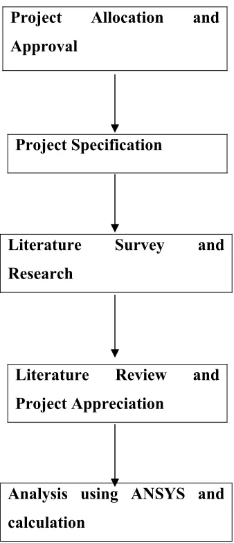
1.3 Project Methodology
The execution of the research project is planned in several stages. After the project is allocated and approved by the examiner and staff of ENG4111, the next step is to specify the details of the project such as the objectives, the requirements and the plan for the project workload. At the same time, research and literature survey are carried out to find the background of the evolutionary structural optimization and other information related to the project.
review summarize the ESO method to multi-component system with a range of design criteria as (1) minimum utilization of materials, (2) maximum overall stiffness, (3) minimum stress and (4) control of natural frequency. Besides that, information on the industrial applications of ESO is equally important to make use of their advantages to the design project.
Thirdly, Modeling of the inter-connection of the analysis is set as a reference for the application of Evolutionary Structural Optimization method. Other than that, it is necessary to have a methodology that can address the design of multi-component systems and generate designs for the optimal layouts of individual structures and locations for interconnections. This is because structural optimization methods for continuum structures consider the design of mainly single structural components. However, in most real life engineering design problems involve multiple components or structures; it is a subject of great relevance. In general, the designs of the individual components are usually coupled. The changes made in the design of one component may influence the design of a multi-component system into design of single components.
For the calculation and analysis part, software ANSYS is used to assist in the calculation of the connected structure analysis. An Evolutionary Structural Optimization (ESO) has been developed and implemented to provide the engineering design community with an alternative optimization technique whereby traditional mathematical programming based optimal processes is replaced by a simple heuristic approach. By progressively eliminating certain amount of under-utilized connection elements to the over-utilized regions, the structures evolve towards an optimum. The ESO method provides significant simplicity in its computer implementation such as ANSYS programming. A great number of numerical examples in a wide range of engineering and physical disciplines have demonstrated the ESO method to be very effective and robust.
In this project the analysis of this method will be carried out to apply on the interconnection of various shapes that stated. To prove the effective in dealing with a variety of design criteria, this technique will be applied on the design of middle pillar to rocker joint to demonstrate the industrial applications.
Stiffness is one of the key factors that need to be taken into account in the design of structures. It is often required that a structure be stiff enough so that the maximum deflection is within a prescribed limit. Hence, this method involves a single cycle of a finite element analysis and continued with a rule driven element removal process without sacrificing the structural performance of the joint to lead the optimal interconnection elements as close to a uniform performance as possible. This reduction of spot-welds has a significant effect on the design considering each spot-weld can cost several thousands of dollars in an assembly line each year.
The order methodology of this project as explained above is illustrated in the schematic diagram, Figure 1
[image:14.612.196.365.295.686.2]Project Allocation and Approval
Figure 1 – Project Methodology Project Specification
Literature Survey and Research
Literature Review and Project Appreciation
Chapter 2
LITERATURE REVIEW
2.1 Background Information
2.1.1 Physical Concept of ESO
Evolutionary structural optimization (ESO) is the method to produce optimal structure by progressively removing a certain amount of under-utilized material from regions of low stress or adding some material to over-utilized regions by a mesh of finite elements. This chapter develops a systematic procedure for the positioning of fasteners within the connection design space which is constructed by the finite element method (FE). At the same time as considering fastener location, the conventional ESO process can be applied to the components being connected, thereby producing an overall approach to the topology optimization of a multi-component structure.
Locations and patterns of connections in a structural system that consists of multiple components can strongly affect its performance. There are mainly two approaches for topology optimization of continuum structures, namely, homogenization and density method (Jiang and Chirehdast, 1997). The premise of the homogenization method is to compute an optimal distribution of microstructures in a given design domain. In other words, the main idea of the homogenization method is to replace the difficult “layout” problem of material distribution by a much easier “sizing” problem for the density and effective properties of a perforated composite material obtained by cutting small holes in the original homogeneous material. The premise of density method is to compute an optimal distribution of an isotropic material where the material densities are treated as design variables. The density method is used to formulate the topology optimization problem for connections. Almost the entire work in the area of topology optimization, however, has been for a single component.
connections. In order to extend the usage life and performance of a structure, it is significant to make sure that the loads borne by the connections are distributed as uniformly as possible.
Presently, structural optimization methods for continuum structures consider the design of mainly single structural components. However, most real life engineering design problems involve multiple components or structures. For present investigation, finite element based optimization of structural systems is proposed and performed in a single structural components or multiple components of trusses, beams and frames. A single changes made in the design of one component may influence the design of a multi-component system or the whole structure of design. Therefore, it is necessary to have a methodology that can address the design of multi-component systems and generate designs for the optimal layouts of individual structures and locations for interconnections.
Choosing a topology is the first step in structural design; it is therefore the layout optimization that is important in the optimal design of structures. It should be connected to one or more redesigned polygon-shaped components to maximize the stiffness of the entire ensemble. One of the methods used is called the homogenization-based design method. It has the ability to change the topology smoothly with a fixed reference domain. A number of objective criteria including stiffness, strength, natural frequency, flexibility, dynamic response, and stability have been used in the application of this method to structural optimization. Besides, an optimality criteria method combined with the steepest descent method also was used to minimize the mean compliance to obtain the stiffest structure for a given volume of material for the connecting structure.
2.1.2 Modeling
The optimization approach is stress-based selecting low and high stressed regions as the areas to be modified. In other words, the connection failure may be caused by an excessive of stress or strain, and an inappropriate allocation of interconnections. In a multi-component system, it is frequently found that failure occurs either at the connection itself or around the attachment regions in the connected components. It may reflect an inefficient use of the connection material, when the low stress or strain is applied.
both, standard analytical shapes and free form shapes. Furthermore, it provides the flexibility to design a large variety of shapes which can be evaluated reasonably fast by numerically stable and accurate algorithms. NURBS are defined by control points which become the design variables of the problem.
The main steps of the basic algorithm are summaries as follows:
Step 1 : The shape or geometry of the structure is defined with load and constraints application.
Step 2 : A boundary element analysis (BEA) is carried out.
Step 3 : Material removal process is performed by selecting the least stressed nodes within the boundary mesh and effectively moving the control points nearest to those nodes. At the same time, material addition is carried out if a node is found with a stress higher than the yield stress or a certain maximum stress
criterion. This satisfies the objective of this project where to remove a certain amount of under-utilized material from regions of low stress or adding some
material to over-utilized regions by a mesh of finite elements.
Step 4 : Finally, such a procedure is repeated, from Step 2, until the evolution of the objective function shows no improvements.
2.1.3 The main steps of the basic algorithm
2.1.3.1 Geometry Definition
intermediate step between design and non-design domain. These three types of lines maybe defined as the intersection between analytical shapes (planes, spheres, cylinders or cones) or grouped together to form combined lines. Furthermore, these lines can be split (or joined) using the cursor and defined as a fillet between 2 existing lines.
2.1.3.2 Boundary element model
The boundary element method is derived through the discretisation of an integral equation that is mathematically equivalent to the original partial differential equation. The boundary surface is divided into elements, thus the essential re-formulation of the partial differential equations that underlies the BEM consists of an integral equation that is defined on the boundary of the domain and an integral that relates the boundary solution to the solution at points in the domain. The advantage of this method relates to the mesh since only the surface of the structure needs to be discretised.
2.1.3.3Removal and addition of material
If the efficiency of a connection element is lower than a threshold level or a so-called removal ratio RR then this connection element is considered to be relatively structurally less efficient. Therefore, it should be removed from the specific connection region. The material can be removed from the structure if any node p satisfies
σ
p≤RR
σ
max (1)and added to the structure if any node p satisfies
σ
p≥σ
y ORσ
p≥AR
σ
max (2)where
σ
p is the node von Mises stress or any other selected criterion,σ
max is the maximumvon Mises stress or any other selected criterion, which varies as the optimization progresses. Is the yield stress or any other maximum tress criterion and AR is the addition ration (0 ≤
RR, AR ≤ 1).
When the removal cycle is repeated by using the same value of RRss, an ESO steady state
that can be removed. An ESO steady state means the lowest efficiency within a specific connection region has become higher than a certain percentage of RRss. To advance such as
optimization process, an evolutionary rate (ER) is introduced and added to RRas
RR
ss+1 =RR
ss +ER
(3)Chapter 3 Optimization of Interconnection Elements under
Single Load Cases
3.1 Summary
Nowadays many engineering design problems involve multiple components or structures, but in this chapter there are only involves to the single load cases. The component interconnections such as rivets, bolts, springs, spot-welds and others may be used in this design system. It is known that the allocation and design of component interconnections play a crucial role in the entire design system. In this chapter, the evolutionary structural optimization method has been extended to develop connect design problems. This method involves a single cycle of a finite element analysis and continued with a rule driven element removal process. The maximum strain energy has been adopted as the design criterion to lead the optimal interconnection elements as close to a uniform performance as possible. In this chapter, the ANSYS program has been implemented to model and solve the design problems. To demonstrate the capabilities of the proposed procedure, a number of design examples are presented herein.
3.2 Introduction
In past few decades, the design refinement and structural optimization for systems made of single components have been focused. Because there is no determinist process for the design refinement, the traditional method of design is to:
· Start with some initial geometry and material,
· Check it against the functional criteria obtained using deterministic processes, · Update the design until it fulfils those criteria.
This method of control of the design system is driven by a non-deterministic process and will produce a design satisfying the functional criteria. However it may not be so good when measured in commercial terms. It is not unusual for a design to reach the detailed phase before any stress analysis is performed. The resulting iterative cycle of detail drawing and analysis is then extremely laborious and time consuming.
position of the support points and the magnitude of the load cases need to be carefully determined in advance. Obviously, this procedure is useable only when the connection patterns between the components can be identified. As a result, a single component design is really an optimum if the fastener locations and sizes have been decided at the outset of the analysis.
Even though highly efficient mathematical programming and analysis capabilities are available to the designer, the widespread use of structural optimization methods to practical engineering problems is still not a reality. Moreover, most engineering structures consist of more than one component part. In various engineering applications, there are a large number of multi-component design examples such as aircraft structures, machine tools, frames of car bodies, computer cases, and pin joint trusses.
Several aspects such as convention, experience and manufacturing factors play an important role in determining the fastener type, positioning, and proportioning, when tried to design a connection pattern. To achieve a best possible structural performance within the manufacturing constraints, an optimization of interconnection is of great practical significance and is also capable of providing a more reliable solution to the entire multi-component system.
An Evolutionary Structural Optimization (ESO) has been developed and implemented to provide the engineering design community with an alternative optimization technique. By progressively eliminating certain amount of under-utilized connection elements to the over-utilized regions, the structures evolve towards an optimum. The ESO method provides significant simplicity in its computer implementation such as ANSYS programming. A great number of numerical examples in a wide range of engineering and physical disciplines have demonstrated the ESO method to be very effective.
The importance of strain energy can be described in terms of the structural load paths in the vibration mode. When a particular vibration mode stores a large amount of strain energy in a particular structural load path, the frequency and displacement shape of that mode are highly sensitive to changes in the impedance of that load path. Thus, strain energy is a logical choice of criteria in model update mode selection. In the case of structures with dominant global behavior, such as a cantilevered beam, the lowest frequency modes may also contain the best overall distributions of structural strain energy.
The results will show that it is better to choose those modes that store the highest level of total structural strain energy over the entire structure, and specifically those modes that store the highest level of strain energy. This is because by using the highest strain energy as the design criterion, the under utilized material (lower strain energy) can be removed from time to time.
This chapter also develops a systematic procedure for the positioning of fasteners within the connection design space. To consider the fastener locations, the conventional ESO process can be applied to the components being connected, hence the evolutionary design optimization for a single component structure can be produced. Several design examples are presented to demonstrate the efficacy and capabilities of the proposed methodology.
3.3
Stiffness Design Criterion
Stiffness is one of the key factors that need to be taken into account in the design of structures. It is often required that a structure be stiff enough so that the maximum deflection is within a prescribed limit. In this section, it describes the evolutionary structural optimization procedures for the multi-component connections with the stiffness criterion.
In finite element analysis (FEA), the static behavior of a structure is represented by the following equilibrium equation:
[
K] {
u} ={
P}
(3.1)The strain energy of the structure, which is defined as
C = ½
{
P}
T{
u}
(3.2)This equation is commonly used as the inverse measure of the overall stiffness of the structure. C is also known as the mean compliance. It is obvious that maximizing the overall stiffness is the same as minimizing the strain energy.
Consider the removal of the i th element from a structure comprising n finite elements. The stiffness matrix will change by
∆ [
K
] = [
K
*] - [
K
] = - [
K
t]
(3.3)Where
[
K*
]
is the stiffness matrix of the resulting structure after the element removal and[
K
t]
is the stiffness matrix of the i th element. It is assumed that the removal of the element has no effect on the load vector{
P
}.
By ignoring a higher order term, we obtain the change of the displacement vector from Equation (3.1) as{
∆
u}
= - [
K
]
-1∆ [
K
]
{
u}
(3.4)From Equations (3.3) and (3.4) then,
∆C
=½
{
P}
T{
u}
= -
½
{
P}
T[
K
]
-1∆ [
K
]
{
u}
=
½
{
ui}
T[
K
i]
{
ui}
Where
{
ui}
is the displacement vector of the i th element. Thus defineε
i=
½
{
ui}
T[
K
i]
{
ui}
(3.5)noted, in fact, that
εi
is the element strain energy and therefore is always positive. This sensitivity number indicates the change in the strain energy as a result of removing the ith element. In general, each element's contribution to the stiffness of a structure varies from location to location. To achieve a more uniform design of stiffness, the material which contributes the least to the overall stiffness should be removed from the structure.3.4 Evolutionary Structural Optimization Procedure
In a traditional ESO, the optimization starts from a more conservative design, where the fasteners are initially allocated over all possible positions. To achieve the optimal connection pattern, those lowly energy stored (under-utilized) connection elements are gradually removed. Therefore, the relative strain energy of the remaining interconnections becomes more uniform. The relative efficiency of connection elements is given as:
α
i =ε
i/
ε
max (3.6)where
ε
max is the highest strain energy over the connection domain. To eliminate those under-utilized connection elements, the ESO algorithm introduces a simple rejection formula which already stated in chapter 2. If the strain energy of a connection element is lower than a threshold level or a so-called rejection ratio (RR) which is:α
i ≤RR
ss (3.7)This connection element is considered to be relatively less efficient (or underutilized. Therefore, should be eliminated from the specific connection region. To comply with the equation above, a removal cycle is repeated using the same value of
RR
ss , until there are no more interconnection that can be removed. This means that an ESO steady state (SS) has been reached, and the lowest efficiency within a specific connection region has become higher than a certain percentage ofRR
ss. For further step of the optimization process, an evolutionary rate (ER) is introduced and added into RR aswith the increased rejection rate, the iterations take place again until a new steady state is achieved.
In the followings, a detailed optimization procedure can be re-organized for the design optimization of connections:
Step 1: Discrete the component system using an appropriate dense finite element mesh, assign the property type of connection and component elements to a number greater than 0.01, define ESO parameter
ER, RR
0and setSS
= 0.Step 2: Perform a FEA to determine the relative efficiency factor α i =
ε
i/
ε
max of all candidate connection elements as Equations (3.1) to (3.6).Step 3: For all candidate elements, if their relative efficiency satisfies Equation (3.7) then assign their property type to zero, and it will be removed from the system.
Step 4: If the steady state is reached,
RR
ss has to increase byER
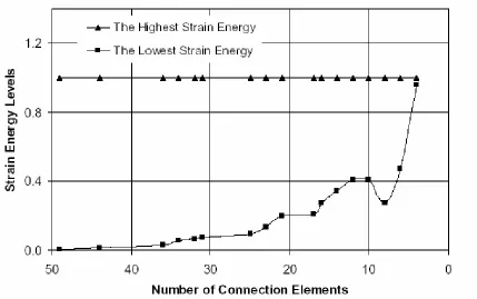
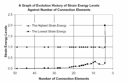
, as in Equation (3.8), and set SS = SS + 1, repeat Step 3; or else, repeat Steps 2 to 3 until the optimal connection pattern is achieved.Besides, the optimal connection patterns also can be determined by plotting a graph of strain energy levels against number of connection elements. The difference of strain energy levels are represented by the highest and the lowest strain energy, in which it can be readily find out by using Equation (3.6). ANSYS program has been used to contribute to the three dimensional finite element analysis for the entire evolution process.
3.5 Design Example
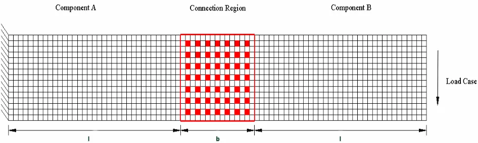
a 15 x 15 grid as shown in Figure 3.1, where the b and l are the dimensions of 150mm and 350mm respectively. 7 x 7 candidate interconnections are modeled by eight-node brick with 30 percent of the thickness and 210GPa of the Young’s modulus of the plates. In all the evolutionary optimization processes of the design cases, an initial rejection ratio of RR0 = 0 and an evolution rate of ER = 1% have been adopted.
3.5.1 Straight Connection Case
In this design example, two components A and B is connected together as in a straight direction. Figure 3.1 shows the initial model of straight overlapped connection, in which the load case is applied in the lower corner of the free end. Figures 3.2 (a) to (p) show the different connection patterns in each iteration of ESO steady state in the evolution process. As the rejection ratio (RR) increases iteration by iteration, the interconnection elements are removed from the candidate location. At the fifth iteration (also the steady state) of the evolution process, there are eighteen interconnection elements removed as shown in Figure 3.2 (f). There are sixteen interconnection elements left when the evolution process reached at tenth iteration as shown in Figure 3.2 (k). It can be found that, by the end of the evolutionary process or at the fifteenth iteration, the optimal interconnection elements are allocated at the four outmost corners of the overlapping square as shown in Figure 3.2 (p). This result could be adopted as a form of validation of ESO process used in connection optimization design problems.
Figure 3.2 ESO connection patterns in the straight joint
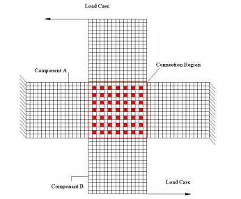
[image:28.612.93.522.428.697.2]3.5.2 Crossover Connection Case
[image:29.612.128.474.389.675.2]Figure 3.5 ESO connection patterns in the crossover joint
[image:30.612.98.527.353.636.2]3.5.3 L- Shaped Connection Case
[image:31.612.129.422.427.692.2]Figure 3.9 The evolution history of strain energy levels of the L-Shaped joint optimization
3.5.4 T-Shaped Connection Case
shows in Figure 3.12 demonstrates that the optimal interconnection occurred at the number of connection element equal to four, in which the highest strain energy levels approach to the lowest strain energy levels.
Figure 3.11 ESO solutions for T-connection patterns
[image:35.612.91.516.306.550.2]3.5.5. U-Shaped Connection
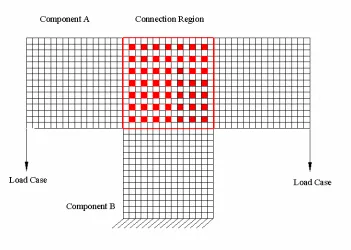
This design example consists of three components A, B, and C, and two groups of fasteners, in which two connection regions are optimized simultaneously. Forty nine connection elements have been used to connect each of the connections AB and BC.
A single load case is applied to the upper right end of the component C, and the entire structure is supported by component A as shown in Figure 3.13. There are several connection patterns achieved at different ESO steady state as in Figures 3.14 (a) to (g). For example, at the third iteration, the connection elements reduced to twenty three at the first connection region and twenty six at the second connection region as in Figure 3.14 (b). At the fifteenth iteration, thirty five connection elements at the first connection region and thirty six connection elements at the second connection region have been removed as shown in Figure 3.14 (d). It is found that the optimal connection pattern of this joint element consists of three interconnection elements in each connection region as in Figure 3.14 (g). The positions of the interconnection elements of both the connection regions are different, this may cause by a vary load case applied at different direction.
Chapter 4 Optimization of Interconnection Elements under Multi
Load Cases
4.1 Summary
Engineering design problems involve multiple components or structures. Moreover, there are more than single load applied on the designed components of the structure. In this chapter, two load cases have been applied to the design examples, and the evolutionary structural optimization method also has been extended to develop for such multiple load cases design problems. Hence, most of the procedures are similar to the previous chapter. Maximum strain energy also has been adopted as a design criterion to have the interconnection elements as close to a uniform load as possible. To achieve the optimal connection patterns, the ANSYS program has been implemented. Some examples are demonstrated in the following.
4.2 Introduction
In recent years, structural optimization has become the focus of the structural design community and has been researched and applied widely both in academia and industry. However, most engineering structures consist of more than one component or structural part. Traditionally, multi-component systems with multiple load cases are usually analyzed at the level of individual components in order to simplify the modeling and design process. In that analysis, the interconnections are treated as some form of sub-boundaries with appropriate load transfer. In this chapter, however, multiple load cases have been taken into account seek for the optimization of interconnection elements. The position of the support points and the magnitude of the load cases also need to be carefully determined in advance for multi-component analyses.
An Evolutionary Structural Optimization (ESO) also has been developed and implemented to provide the engineering design community with an alternative optimization technique whereby traditional mathematical programming based optimal processes is replaced by a simple heuristic approach. By progressively removing a certain amount of under-utilized material or adding some material to over-utilized regions, the structure evolves towards an optimum. Similarly to previous structural optimization methods, this chapter considers multiple load cases instead of single load cases to the entire design examples. A strain energy based approach is proposed to design a fastener layout that achieves an almost uniform strain energy level in each interconnection element. With the ESO method, the connection element itself, rather than its associated physical parameters, such as the stiffness, is treated as the design variable. Three design examples are presented to demonstrate the capabilities and efficacy of the proposed methodology.
4.3 Stiffness Design Criterion
Stiffness design criterion for multi-load cases is similar to the previous single load case. It is often required that a structure is stiff enough so that the maximum deflection is within a prescribed limit. This chapter also describes the evolutionary structural optimization procedures for the component connection with the stiffness criterion, in which multi-load cases are involved.
At a more complex but realistic level, where the multi-component system may be operated under circumstances involving multiple load cases, as governed by the finite element equation:
[K] {
u
k} = {
P
k} ( k = 1,2,….LCN)
(4.1)
the relative efficiency under all the load cases can be estimated by a weighted average scheme as:
or by an extreme value scheme as:
(4.3)
where, LCN denoted the total number of load cases, { P k } ( k = 1,2,….LCN) the vector of
the kth load case,
ε
i C (Pk) the von Mises strain energy of the ith connection element underthe kth load case, w(Pk) gives the weighting factor for the kth load case, calculates
the highest strain energy level of the ith connection under all load cases and calculates the highest strain energy level at all load cases LCN over all interconnections Mt in the tth connection region. For convenience, the former is termed as the
overall efficiency and the latter is named as the extreme efficiency. The efficiency factor provides a criterion to justify which connection elements should remain and which ones should be eliminated.
The formulations in Equations (4.1)-(4.3) could treat various connection regions differently. This means that the goal of equal efficiency can be sought in individual connection regions. This provides a way of dealing with different connection types and sizes. On other hand, if the desired connection type and size among all connection regions are the same, the global maximum strain of all regions
(4.4)
4.4 Evolutionary Structural Optimization Procedures
Similarly to the previous chapter of single load cases, to achieve the optimal connection pattern, those inefficiency connection elements are gradually removed. It is therefore, the relative efficiencies of the remaining interconnections become more uniform. Hence, the ESO algorithm introduces a simple rejection formula to eliminate those under-utilized connection elements. If the relative strain energy of a connection element is lower than a threshold level or a so-called rejection ratio (RR), which is:
α
i ≤RR
ss(
i =
1,2….., M) ( t = 1,2,….T)
(4.5)
then this connection element is considered to be relatively less efficient, and therefore, should be eliminated from the specific connection region t, To comply with the equation above, a removal cycle is repeated using the same value of
RR
ss until there are no more interconnection that can be removed. This means that an ESO steady state (SS) has been reached, and the lowest efficiency within a specific connection region has become higher than a certain percentage ofRR
ss. For further step of the optimization process, an evolutionary rate (ER) is introduced and added into RR asRR
ss +1=RR
ss+ ER
(4.6)
with the increased of rejection rate, the iterations take place again until a new steady state is achieved.
The following optimization procedures can be determined for the design of\ connections for multi load cases as well:
Step 1: Discrete the component system using an appropriate dense finite element mesh define ESO parameter ER, RR0 and set SS = 0.
Step 2: Perform a FEA to determine the relative efficiency factor of all candidate connection elements as Equations (4.2) to (4.4).
Step 4: If the steady state is reached,
RR
ss has to increase by ER, as in Equation(4.6), and set SS = SS + 1, repeat Step 3; or else, repeat Steps 2 to 3 until the optimal connection pattern is achieved.
Basically, the difference in this chapter compare with the previous chapter is that the average of the highest strain energy on both design structures with the different load cases direction have been taken to solve for the entire process, and the rest of the procedures is similar.
4.5 Design Examples
In this chapter, several typical connection designs are investigated. Such as an L-shaped connection case, T-L-shaped connection case, and U-L-shaped connection case are demonstrate at the following paragraphs. Although these several design examples are similar compared to the previous chapter, multi-load cases have been used instead of a single load case. Two or three components can be connected in a connection region by using either threaded fasteners, rivets, pins or spot welds. These connection elements can be represented by brick elements, in which it is meshed with a 15 x 15 grid as shown in Figure 4.1, where the b and l are the dimensions of 150mm and 450mm respectively. There are 7 x 7 candidate interconnections are modeled by eight-node brick with 30 percent of the thickness and 210GPa of the Young modulus of the plate. In all evolutionary optimization processes of the design cases, an initial rejection ratio of RR0 =0 and an evolution rate of ER = 1 percent have
been adopted.
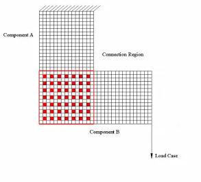
4.5.1 L-Shaped Connection Case
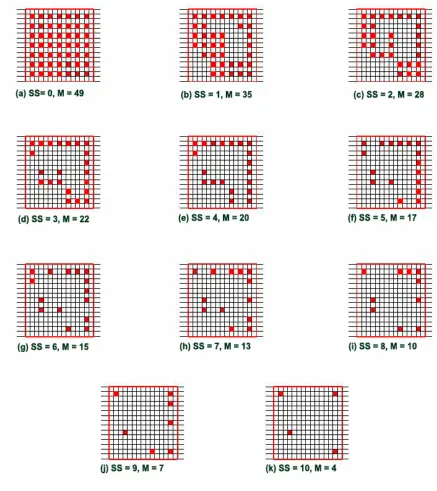
inefficient connection elements are removed from candidate locations. Figures 4.2 (d), (e), and (f) show that the major number of inefficient connection elements eliminated are allocated at the lower right corner of the connection region. There are only eleven connection elements left at sixteenth iteration, and reduced to six when twentieth iteration is reached as shown in Figures 4.2 (i) and (k) respectively. It is found that the optimal connection pattern at ESO steady state is achieved at SS = 17, and there are only four connection elements left as illustrated in Figure 4.2 (l). This result could be argued to be some form of validation of the ESO process implemented in connection optimization problem.
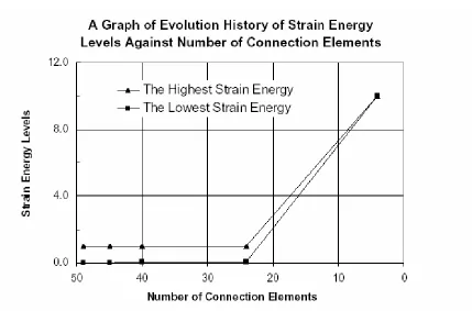
Again, the evolution process can be monitored by plotting a graph of strain energy levels against number of connection elements as shown in Figure 3.3. From the evolution history curves, the point of the highest strain energy approaches to the lowest strain energy during optimization process. The highest and the lowest strain energy in the surviving connection elements become smaller and smaller with the evolution process, which reflects a path approaching a fully strain energy design.
[image:45.612.71.584.381.626.2]Figure 4.3 The evolution history of strain energy levels of the L-shaped joint optimization
4.5.2 T-Shaped Connection Case
There is only eight connection elements left at eleventh steady state as in Figure 4.5 (l). It demonstrates that when the steady state is increased more and more, the number of connection elements will be eliminated. However, the optimal connection pattern is achieved at the twelfth iteration, which the last survived connection elements locate at the four outmost corners of the overlapping square as shown in Figure 4.5 (m). It is found that the allocation of eight connection elements around the edges of the connection domain does not offer the optimum in the connection pattern.
From the evolution histories of strain energy deviation, one can identify the optimal connection patterns. It can readily find out that the minimum difference between the highest and the lowest strain energy points occur at four interconnections from Figure 4.6. This explores that the connection pattern M is the best strength efficiency performance compared with the performances of eight and ten connection elements.
[image:48.612.61.589.366.568.2](a) Load case acted on left direction (b) Load case acted on right direction
Figure 4.6 The evolution history of strain energy levels of the T-shaped joint optimization
4.5.3 U-Shaped Connection Case
The third design example is a U-shaped connection case. This connection case consists of three plates A, B and C as illustrated in Figure 4.7, in which two connection regions are optimized simultaneously. Basically, this design example is similar to L-shaped connection case; the only difference is that another connection region is added (M1 = M2 =
(a) Load case acted on right direction
[image:51.612.111.513.73.337.2]Figure 4.8 shows the ESO solution connection patterns at different steady states. At the first iteration, it could be seen there is more inefficient connection elements are eliminated start from the end corner of each connection region as in Figure 4.8 (b). To due with multi-load cases, the inefficient connection elements in both connection regions removed simultaneously. In Figure 4.8 (d), twenty one connection elements are removed in each connection regions at the sixth iteration. When the ESO steady state reached the twelfth, more inefficient connection elements have been eliminated, in which only seventeen connection elements are left in each connection regions as shown in Figure 4.8 (f). There are only six connection elements left in both connection regions when the ESO steady state increases to twenty-first as shown in Figure 4.8 (i). The optimal connection pattern for the U shaped connection case is shown in Figure 4.8 (j), in which the number of last survived connection elements equal to four in each connection regions. This indicates the surviving interconnections have both higher extreme efficiency and the higher over all efficiency for these two load cases.
Chapter 5 Conclusion
Up to this stage of the analysis, results show that the importance of Evolutionary Structural Optimization in the industrial area and every engineering discipline. By following the ESO procedure, the inefficient elements are gradually removed from the regions which are in lower stress and it will be improve by distributing the strain energy as uniform as possible at the region of the interconnection. From the strain energy deviation graph which is showing the history of evolution of strain energy levels of the every joint optimization. The result of the deviation graph is able to tell whether the solution that obtained is accepted.
In the analysis of optimization, highest strain energy has been adopted as the design criterion as what has been discussed in the earlier chapter. There are several researches on the Evolutionary Structural Optimization where the stress level of the interconnection has been assigned as the design criterion. In comparing these two methods of optimization, these two methods give more or less the same results for the interconnections that analyzed in this project.
This paper extends the evolutionary structural optimization method to the design of multi-component systems, which involves both single load cases and multiple load cases. To have the interconnection elements carry as uniform strain energy as possible, strain energy levels of all candidate connection elements are employed to estimate the relative performance. The absence and presence of an interconnection is determined in terms of its relative performance of stiffness by complying with this concept. In the optimization process, those inefficient connection elements are gradually removed from the structural system by following the evolutionary structural optimization procedures. This significantly simplifies the optimization process and makes the algorithm easy to be applied into different design problems.
REFERENCES AND FURTHER READING
1. Bendsoe, M.P., Kikuchi, N. (1998). Generating optimal topologies in structural design using a homogenization method. Computer Methods in Applied Mechanics and Engineering 71:197-224.
2. Chickermane, H. and Gea, H.C. (1997), Design of multi-component structural systems for optimal layout topology and joint locations, Engineering with Computers, Vol. 13, pp. 235-43.
3. Chickermane, H., Gea, H.C., Yang, R.J. and Chung, C.H. (1999), Optimal fastener pattern design considering bearing loads, Structural Optimization, Vol. 17 pp. 140-6
4. David Roylance. (2001), Finite Element Analysis, Department of Materials Science and Engineering, Massachusetts Institute of Technology Cambridge, MA 02139 5. E. Cervera, J. Trevelyan. (2005), Evolutionary structural optimization based on
boundary representation of NURBS. Part I: 2D algorithms, Computers and Structures 83 1902–1916
6. E. Cervera, J. Trevelyan. (2005), Evolutionary structural optimization based on boundary representation of NURBS. Part II: 3D algorithms, Computers and Structures 83 1917–1929
7. Jiang, T. and Chirehdast, M. (1997, A system approach to structural topology optimization: designing optimal connections, ASME Transactions: Journal of Mechanical Design, Vol.119, pp.40-7.
8. John Barlow. (2000), Structural Design Optimization In The Real Engineering World, PTC.
9. L. Fryba and J. Naprstek (Eds.); A.A. Balkema, Rotterdam. (1999), Structural Dynamics EURODYN’99, Engineering Structure, pp 1224–1226
10.Li, Q., Steven, G.P. and Xie, Y.M. (2001), Evolutionary structural optimization for connection topology design of multi-component systems, to appear in Structural Optimization.
11.Pasi Tanskanen, (2002), The evolutionary structural optimization method: theoretical aspects, Computer. Methods in Applied in Mechanical and Engineering. pp.5485– 5498
13.Xie, Y.M. and Steven, G.P. (1994), optimal design of multiple load case structures using an evolutionary procedure, Engineering Computations, Vol. 11. pp. 295-302. 14.Xie, Y.M. and Steven, G.P. (1997), Evolutionary Structural Optimization,
Springer-Verlag, Berlin.
Appendix
ANSYS GUI Program
To build a structure design: (straight connection case)
Start with new Analysis Preferences
Click Structural OK
Pre-processor
Element type
Add/Edit/Delete Add
(Solid) & (Brick & node 185) CLOSE
Material Props
Material Models
Material Model number 1 Structural Linear Elastic Isotropic
EX = 210E9 PRXY = 0.3 OK
Edit
Copy OK
Material Model number 2 Linear Isotropic
EX = IE + 011 PRXY = 0.3 OK
X Exit
Modelling Create
Volumes
Block By dimensions
X1 , X2 = 0, 0.45
Y1 , Y2 = 0, 0.15 - APPLY
X1 , X2 = 0.3 , 0.45
Y1 , Y2 = 0 , 0.15 - APPLY
Z1 , Z2 = 0.01 , 0.015
X1, X2 = 0.3 , 0.75
Y1, Y2 = 0 , 0.15 - OK
Z1 , Z2 = 0.015 , 0.025
Operate
Booleans Glue
Volumes 9 Pick All
Plot Operate
Specified Entities Volume 1, 4, 1
OK
Create
Volumes
Block By dimensions
X1 , X2= 0.3 , 0.31
Y1 , Y2 = 0 , 0.15 - APPLY
Z1 , Z2 = 0.01 , 0.015
X1 , X2= 0.3 , 0.45
Y1 , Y2 = 0.14 , 0.15 - OK
Z1 , Z2 = 0.01 , 0.015
Copy
Volume Pick horizontal OK
8, 0.02, 0, 0 no. of copies, DX, DY, D OK
Copy
Volume Pick vertical OK
8, 0,-0.02, 0 OK
Operate
Booleans
Pick all &
OK
Glue
Volumes Pick all
Meshing
Mesh tool Element Atrriutes : Volumes SET 6 Pick 1&2 plates
OK
Material number = 1 Apply
Pick all elements OK
Material number = 2 OK
Mesh tool size controls: Global SET
Size element = 0.01 No. of element = 0
OK
Lines SET
Pick DY for 1 & 2 place OK
Size element = 0.01 No. of elements =15 Size , NOIV = NO
APPLY
Pick DX for 1&2 place OK
Size element = 0.01 No. of elements = 45 SIZE, NOIV = NO APPLY
Pick DE for 1 & 2 place OK
Mesh tool
Mesh : volumes
Shape : HEX/Wedge :Sweep SWEEP
Pick for 1&2 place OK
Plot
Specified Entities Volume 1, 68, 1 Mesh tool
Lines SET
Pick all DX, DY for all elements OK
Size element = 0.01 No. of elements = 45 SIZE, NOIV = NO
APPLY
Pick DZ for all element OK
Size element = 0.005 No. of elements = 1 SIZE, NOIV = NO
OK
Mesh tool
Mesh : volumes Shape : HEX/Wedge :Sweep
SWEEP
Pick all elements OK
To apply load cases: Solutions
Define loads
Apply Structural Displacement
On areas Pick boundary condition in 1 place OK
DOF1 = All DOF Displacement Value =0
OK Directions = FY Value = -150
OK
(Warning _ CLOSE)
To solve the structure: Solve
Current LS
OK 2 Warning ± CLOSE X exit
General Postproc Plot results
Contour plot
Item be contoured = stress : Von Mises SEQV OK
List Results
Element solution
Energy : strain energy SENE OK
To copy into Excel:
Copy the results from table from 1350 to 1399 Paste in notepad
Open excel
Open the Notepad file Save in excel _ 2 rows
Next
V space
FINISH
From table remove 1372 - 1366
- 1384 - 1360 - 1370
Removing elements Pre-processor
Meshing Clear
Volumes Pick the elements that want to be removed OK
Modelling _ Delete
Volumes only Pick the element that want to be removed OK
PLOT 3 Replot 4)
Solution _ solve
Currene LS _ warning CLOSE X exit
General postproc _ list results
Element solution _ energy : strain energy SENE OK
FEA diagrams haven been taken using ANSYS program Single load case design example for Straight Connection Case At the initial state
At Isometric View
Multiple load cases design example for L-shaped Connection Cases At the initial state
a. The force applied to downward direction
At Oblique View
a. The force applied to downward direction
At Front View
b. The force applied to upward direction
At the final state
a. The force applied to downward direction b. The force applied to upward direction At Oblique View