Daily streamflow analysis based on a two-scaled gamma pulse model

This is a repository copy of

Daily streamflow analysis based on a two-scaled gamma pulse

model

.

White Rose Research Online URL for this paper:

http://eprints.whiterose.ac.uk/78943/

Article:

Muneepeerakul, R, Azaele, S, Botter, G et al. (2 more authors) (2010) Daily streamflow

analysis based on a two-scaled gamma pulse model. Water Resources Research, 46 (11).

W11546. ISSN 0043-1397

https://doi.org/10.1029/2010WR009286

[email protected] https://eprints.whiterose.ac.uk/

Reuse See Attached

Takedown

If you consider content in White Rose Research Online to be in breach of UK law, please notify us by

Daily streamflow analysis based on a two

‐

scaled gamma

pulse model

Rachata Muneepeerakul,

Sandro Azaele,

Gianluca Botter,

Andrea Rinaldo,

and Ignacio Rodriguez

‐

Iturbe

Received 10 March 2010; accepted 13 August 2010; published 23 November 2010.

[1]

In this paper, we develop a simple analysis method to infer some properties of the

watershed processes from daily streamflow data. The method is built on a simple streamflow

model with a link to rainfall stochasticity, which characterizes the streamflow as a series of

overlapping gamma distribution

‐

shaped pulses. The key premise of the method is that the

complex streamflow processes can be effectively captured by simply dividing streamflow

into two regimes. Specifically in this method, the gamma pulse model is applied separately to

low

‐

and high

‐

flow regimes. We demonstrate the application of the method to five

watersheds and show that it is capable of capturing at least two important statistical

properties of streamflow, namely the probability density function and the autocorrelation

function for wide ranges of values (i.e., from low to large flows and time lags, respectively).

Citation: Muneepeerakul, R., S. Azaele, G. Botter, A. Rinaldo, and I. Rodriguez‐Iturbe (2010), Daily streamflow analysis based on a two_‐scaled gamma pulse model,Water Resour. Res.,46, W11546, doi:10.1029/2010WR009286.

1.

Introduction

[2] Streamflow is one of the most influential hydrological

phenomena affecting human well‐being. It provides the most easily accessible source of water, but it can also produce severe damages via flooding. Less directly but importantly, it governs functions and services of numerous types of ecosystems upon which human rely. Scientifically, it poses fascinating questions because it results from various hydro-logical processes operating at a wide range of spatial and temporal scales [e.g.,Bras and Rodriguez‐Iturbe, 1993;Xu et al., 2002;Van de Griend et al., 2002;Farmer et al., 2003; Kirchner, 2009; Botter et al., 2009]. Deservedly, there is a long history of studies of the dynamics governing streamflow fluctuations [e.g.,Weiss, 1977;Rodriguez‐Iturbe and Valdes, 1979;Bras and Rodriguez‐Iturbe, 1993;Beven, 2001; Xu et al., 2002; Claps et al., 2005;Kirchner, 2006, 2009; Botter et al., 2007a, 2009]. Many models that are devised to link rainfall to streamflow, e.g., traditional rainfall‐ runoff models, do so through a case‐by‐case type of rep-resentation with a large number of parameters and the corresponding calibration. While extremely useful for their purposes, most of these models may not lend themselves to general conclusions applicable to a number of ecosystems

closely connected to streamflow, e.g., riparian zones and certain classes of wetlands [see, e.g.,Camporeale and Ridolfi, 2006;Muneepeerakul et al., 2007;Perona et al., 2009].

[3] Central to this paper are two important issues in

studying streamflow. First, we address the issue of the probabilistic structure of streamflow time series with an explicit link to rainfall stochasticity. It is worth noting that this issue has in fact been partially addressed in the studies byBotter et al.[2007a] andBotter et al.[2009], where the probability density function (pdf ) of the slow, subsurface component of the streamflow, i.e., base flow, was derived. The key assumption in these works is that the streamflow is a unique function, either linear [e.g.,Botter et al., 2007a] or nonlinear [e.g.,Kirchner, 2009;Botter et al., 2009], of the water storage in the watershed. Indeed,Botter et al.[2007b, 2009] show that when the base flow constitutes a major contribution of the overall streamflow, the derived pdf pro-vides a good approximation of the streamflow pdf over the low‐flow range.

[4] Here, we consider an alternative approach, namely to

represent the streamflow time series by a series of over-lapping gamma‐shaped pulses [see, e.g.,Xu et al., 2002]. The use of overlapping pulses to represent a stochastic phenom-enon has previously been employed for rainfall dynamics [Rodriguez‐Iturbe et al., 1984, 1987, 1988]. Therein, the pulses took a simple rectangular shape and many important properties of the rainfall dynamics were analytically derived. As will be shown later, an important advantage of this for-mulation is that it enables us to study another crucial aspect of the streamflow probabilistic structure, namely its autocorre-lation function.

[5] Second, we investigate the issue of time scale

differ-ence in processes contributing the streamflow. As mentioned above, streamflow results from a suite of complex watershed processes operating at very different spatial and temporal scales, ranging from very slow groundwater flows to fast floods. As such, models or analyses that are built to capture 1_{Department of Civil and Environmental Engineering,}

Princeton University, Princeton, New Jersey, USA.

2_{Now at School of Sustainabilty, Arizona State University, Tempe,} Arizona, USA.

3_{Now at Institute of Integrative and Comparative Biology,} University of Leeds, UK.

4_{Dipartimento di Ingegneria Idraulica, Marittima, Ambientale e} Geotecnica, and Centro Internazionale di Idrologia “Dino Tonini,” Università di Padova, Padua, Italy.

5_{Laboratory of Ecohydrology, Faculte´ ENAC, Ecole Polytechnique} Federale,Lausanne, Switzerland.

processes of a single time scale have a serious disadvantage in adequately representing the entire streamflow process. Indeed, the time scale separation and other complexity in watershed processes continue to fascinate hydrologists and provide a fertile ground for hydrological research [e.g., Xu et al., 2002;Farmer et al., 2003;Kirchner, 2006, 2009; Botter et al., 2009]. Here, we develop a simple application‐ oriented analysis method to address this issue. While it does not deal with the time scale separation mechanistically, the method can be used to extract meaningful insights from streamflow data, which can be used in developing more process‐based and sophisticated models. Let us emphasize here that the method is developed to provide a framework in which one can quantitatively infer various components of streamflow processes from daily streamflow data, not to make predictions; such tasks call for more process‐based models.

[6] The paper is organized as follows. In section 2, we

construct the gamma pulse model for streamflow in a generic way. In section 3, a method is built on the pulse model and its application to empirical daily streamflow data is demon-strated; in brief, the pulse model is applied to two different flow regimes of very different time scales, yielding very satisfactory overall results. Conclusions, discussion, and final remarks are presented in section 4.

2.

Gamma Pulse Model for Streamflow

[7] We approximate the watershed response, h(u), of a

watershed by a gamma distribution [see, e.g.,Nash, 1957]. h(u) is the response, i.e., streamflow, of a watershed to a unit volume of water input applied uniformly and instanta-neously over the watershed. It is conceptually very similar to the familiar instantaneous unit hydrograph. However, the unit hydrograph is typically used to describe only the

sur-face runoff component of the streamflow. We thus avoid the use of the term and potential confusion.

[8] A gamma‐shapedh(u) can be expressed as:

h uð Þ ¼ b

Gð Þa ð Þbu

a 1

e bu;u0_{; ð}1_Þ

where u is the time after the arrival of a streamflow‐ generating rainfall event; a and b are the shape and scale parameters of the gamma distribution, respectively; andG(·) represents the gamma function. Equation (1) satisfies the conditionR

0

∞_{h(u)du= 1. Accordingly, the time to peak of}

h(u),tp= (a−1)/bwhena> 1 and 0 otherwise. Note that the time scale of the observed streamflow data is critical to the interpretation oftp.

[9] Under this formulation, the streamflow is simply a

result of overlapping gamma pulses, each of which is trig-gered by a streamflow‐generating rainfall event. Now, it has been shown that at a daily time scale, the rainfall dynamics can be properly modeled as a marked Poisson process [e.g., Rodriguez‐Iturbe and Porporato, 2004]: specifically, the arrival of rainfall events may be assumed a Poisson process with ratelPand the daily rainfall depth being an exponen-tially distributed random variable with the mean depthmP. The analysis of rainfall data used in this study confirms the validity of this assumption (results not shown).In addition, since not all rainfall events generate streamflow, we assume that only those with depths larger than a thresholdDdo so. Note that under the current framework,Dis assumed fixed and can be thought of as a long‐term average value since we are considering the statistical properties of long stream-flow time series, not of a single event (but see also, e.g., Botter et al. [2007a, 2007b] and discussion in section 4). Consequently, the arrival of streamflow‐generating rainfall events can be modeled as a Poisson process with ratel=

lP exp(−D/mP) with the depth of each event remaining exponentially distributed with the same meanmP[Rodriguez‐ Iturbe et al., 1999;Rodriguez‐Iturbe and Porporato, 2004]. [10] Let Q(t) be the streamflow at time t, which can be

written as [see, e.g.,Cox and Isham, 1980;Rodriguez‐Iturbe et al., 1987]:

Q tð Þ ¼ Z t

1

h tð zÞV zð ÞdN zð Þ; ð2_Þ

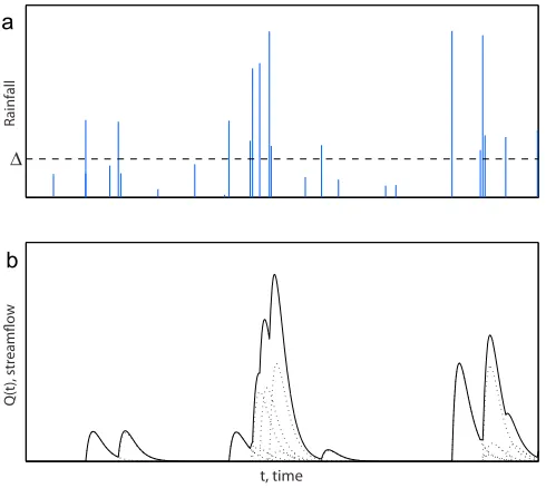
where V(z) is the random streamflow volume generated by a rainfall event arriving at time z and {N(z)} counts the occurrences of the Poisson process representing the arrivals of streamflow‐generating rainfall events. Note that equation 2 is dimensionally consistent as the dimensions ofQ,h, andV are [L3/T], [1/T], and [L3], respectively. Based on the above formulation, V is exponentially distributed with the mean volume mV = mPA, where A is the drainage area of the watershed under consideration. The illustration of Q(t) and its relation to the rainfall process is shown in Figure 1.

[11] We then derive the meanmQand variancesQ2 of the

processQ(t) as:

Q¼EfVg Z 1

0

h uð Þdu¼V; ð3Þ

2_Q¼EfV2g Z 1

0

h2ð Þudu¼2_V b

G að Þ; ð4Þ Figure 1. Illustration of a series of overlapping gamma

pulses representing streamflow: (a) rainfall and (b) stream-flow. In Figure 1b, the dotted lines represent the gamma‐ shaped pulses generated by rainfall events in Figure 1a that are larger thanD, and the solid line represents the resulting streamflow, which is the sum of all dotted lines.

MUNEEPEERAKUL ET AL.: GAMMA PULSE STREAMFLOW ANALYSIS W11546 W11546

where,

G að Þ ¼4 a 1

G_{ð Þ}a2

G_ð2_a 1_Þ; ð5Þ

andE{·} stands for the expectation operator. Another impor-tant property of Q(t) is its autocorrelation as a function of lagt,r(t), which is derived as:

ð Þ ¼CQð Þ 2

Q ¼

R1

0 h uð Þh uð þÞdu

R1

0 h 2

u ð Þdu

¼ ffiffiffiGð Þa

p

G_ð2_a 1_Þð2bÞ a 1

2_K

a 1

2ð Þb ; ð

6_Þ

where CQ(t) = E{(Q(t)− mQ)(Q(t+ t)−mQ)} is the auto-covariance of the streamflow process Q(t) and Kn(·) rep-resents the modified Bessel function of the second kind. Note that due to the independence among rainfall events associated with the Poisson characterization,r(t) depends only onaand b, which specify the shape ofh(u), and not onlandmV.

[12] Finally, while we have not analytically derived the

exact expression of the probability density function (pdf ) of Q,p(q), simulation results suggest that a gamma distri-bution whose mean and variance coincide with equations 3 and 4, respectively, provides an excellent approximation for a wide parameter range. That is,p(q) can be written as:

p qð Þ c

Gð Þ ð Þcq

1

e cq;q0_{; ð}7_Þ

where and care the shape and scale parameters of this gamma approximation of the pdf (not to be confused witha and bassociated withh(u) in equation 1). Rearranging and grouping terms, we writeandcas:

_¼G að Þ

b ; ð8Þ

c¼ 1 V

G a_{ð Þ}

b : ð9Þ

In the special case ofa = 1,h(u) takes an exponential form and = l/b; this is equivalent to the criterion used in the studies by Botter et al.[2007a, 2007b] to classify dry/wet conditions of rivers. In many watersheds, however, gamma distributions withagreater than 1 have been shown to yield reasonable representation of the IUHs; for example, when a = 2, becomes 2l/b. This simply shows that is also closely tied to the shape of h(u).

3.

Analysis Method for Daily Streamflow

Time Series

[14] In section 2, we developed the gamma pulse model for

streamflow in a generic way. To apply it to real data, one must recognize that streamflow results from a suite of complex watershed processes operating at very different spatial and temporal scales. As such, this simple model described above should not be applied directly to the overall streamflow because such a gamma‐shaped pulse only captures processes of a single time scale. We now describe step‐by‐step a simple analysis method, with the gamma pulse model as building

blocks. It is essentially based on a simple premise that dividing streamflows into only two regimes, low‐and high‐ flow, is sufficient to effectively capture the overall process. Note that this method is application‐oriented and approxi-mate in nature, with the focus on practicality and usefulness, and does not mechanistically address the problem of time scale separation. In particular, we will show that it can capture the probability density function (pdf ) and autocorrelation function of the overall streamflow and can subsequently be used to infer relevant information regarding the watershed processes.

[15] The required parameters can be estimated as follows:

[16] Infer the watershed responses responsible for the low_‐ and high‐flow regimes from the autocorrelation function. We first make the following approximate categorization: the low flows determine, by definition, the shape of the low‐ flow part of the streamflow pdf, and more importantly, pre-dominantly contribute to the autocorrelation at large time lags. On the other hand, the high flows determine the tail structure of the streamflow pdf and control the autocorrela-tion at short time lags. Because the difference in time scales between the two flow regimes is generally large, the gamma pulse model is applied to them separately as follows. Note that in many cases, the distinction between the two regimes is quite noticeable in both the pdf and autocorrelation. Here, use is made of the fact thatr(t) (equation (6)) depends solely on the watershed response (i.e., throughaandb). LetaLandbL denote the shape and scale parameters ofhL(u), the watershed response associated with the low‐flow regime; they are esti-mated by finding the values that best fit the empiricalr(t) whentis large, say, larger than 4–6 days. Similarly, letaH andbHdenote the shape and scale parameters ofhH(u), the watershed response associated with the high‐flow regime; they are estimated by finding the values that best fit the empiricalr(t) whentis small, say, within 2 or 3 days.

[17] Separate the two flow regimes. We now determine the

thresholdq*, the threshold streamflow dividing the low‐and high‐flow regimes. Based on equations 3 and 4, the variance‐ to‐mean ratio, or the so‐called Fano factor, of the low flows FLismVbL/G(aL). We simply tuneq*such that the empirical FLmeets this constraint.

[18] Estimate mV and D. mV can be estimated directly from the rainfall data from rain gages in the watershed via the relationshipmV =mPA(section 2). Dcan be estimated by substituting the empirical mean streamflow for lmV (equation (3)) in the following relationship:D=mPln(lPmV/

lmV) (see section 2 and also Botter et al. [2007b, 2008, 2009]).

[19] With these parameters determined, we can compute

other quantities of interest. In particular, with q* and mV known, equation 3 is used for the conditional mean flows to compute the conditional Poisson arrival rates associated with the low‐ and high‐flow regimes, denoted by lL and

lH, respectively. The overall arrival rate of streamflow‐ generating rainfall events, l, can be computed by either applying equation 3 to the mean overall streamflow or using the following relationship:l=fLl′L+ (1−fL)l′H, wherefL= P[Q < q*] is the fraction of time the streamflow process spends in the low‐flow regime. Then, the pdf of overall streamflow can be approximated by:

wherepL(q) andpH(q) are the approximate pdf’s of the low‐ and high‐flow regimes, respectively, which can be expressed as in equation 7 with regime‐specificlr, ar, and br where subscriptris eitherLorH.

[20] We now demonstrate the application of this method

to daily streamflow data from several relatively small water-sheds with different climates and seasonality patterns; their relevant information is reported in Table 1. The fitted param-eters are summarized in Table 2 and the results illustrated in Figures 2–6. The results show that the proposed method can indeed capture both autocorrelation and pdf over entire ranges, except the probability of the extreme high flows in some cases. This suggests that simply dividing streamflow into two regimes is sufficient to effectively capture this com-plex process.

[21] It is important to note that the studied periods were

selected such that there were no strong trends or abrupt changes in the daily streamflow time series and no significant snowfall. The first condition is imposed to be consistent with the assumption of temporal stationarity embedded in the model, while the second is imposed simply because the streamflow generated by snowmelt processes is not captured in the model. Interestingly, the results suggest that the method performs well even when some seasonality, i.e., non-stationarity, exists. Here, we use the coefficient of variation of monthly rainfall, CVMR, to measure the degree of seasonality.

Figures 2–4, along with Table 1, show that the pdf and autocorrelation are well captured when CVMR is as high as

0.37. Furthermore, in the very dry climate of the Californian watershed (Figure 5), the performance is still robust even with CVMR of 1.03. However, the method seems to fail (e.g.,

giving some insensible values) when applied to the entire streamflow time series at sites in a wet climate with pro-nounced seasonality, e.g., the Oregonian watershed in this study, although it still yields good results when applied only to the dry season (Figure 6).

[22] The key contribution of this method is that it allows us

to gain some insights in watershed processes through study-ing the resultstudy-ing parameters. For example, 1/bLand 1/bHcan be interpreted as the characteristic time scales of the low and

high flows, respectively. The huge difference between them, approximately two orders of magnitude in most cases (see Table 2), justifies our scale separation procedure: 1/bHcan be as small as less than a day, while 1/bLcan be close to a year. Clearly, models with a single characteristic scale are not adequate for the streamflow process in these settings. Con-versely, the method can help us identify circumstances under which a simpler single‐scaled approach may be adequate. For example, consider the case of the Oregonian watershed dur-ing the dry season in which the scale and shape parameters of the low‐flow and high‐flow responses are more similar than other case studies. When a single‐regime response (a= 0.889, 1/b = 7.4 days) is employed (results not shown), the auto-correlation and pdf are still captured reasonably well, except that the probability of flow larger than 1 cm/d is more severely underestimated.

[23] The shape parameter of the high‐flow response, aH,

seems to vary within a reasonable range, whereas its low‐flow counterpart,aL, seems to oftentimes be between 0.5 and 0.6. Based on the discussion in section 2, the range of aLmay translate to the interpretation that the time to peak of the low‐flow watershed response is close to zero, i.e., it peaks instantaneously and monotonically decreases afterward. Here, a caveat is in order. Recall that the observed data are at a daily time scale, and thus an important implication is that the rise ofh(u) with tp1 day is likely not captured and only its recession is. This condition is likely the case for these relatively small watersheds. Accordingly, one should only interpret the low values of a as that the watershed response peaks quickly—significantly less than 1 day—but not necessarily instantaneously.

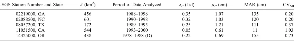
[24] Additionally, the values offLin Table 2 suggest that, while the streamflow processes in these particular examples of small watersheds are in the low‐flow regime for the majority of the time, the infrequent high‐flow regime strongly controls the autocorrelation over short time lags and the tail structure of the streamflow pdf. Finally, D, the threshold beyond which a rainfall event generates streamflow, offers a simple way to collectively characterize and compare streamflow production processes of different watersheds; it Table 1. Summary of Relevant Characteristics of the Two Watersheds Under Considerationa

USGS Station Number and State A(km2) Period of Data Analyzed lP(1/d) mP(cm) MAR (cm) CVMR

02219000, GA 456 1988–1998 0.35 1.07 135 0.20

02088500, NC 601 1990–1998 0.32 1.03 120 0.20

08057200, TX 172 1989–1995 0.25 1.21 111 0.37

11051500, CA 544 1993–2000 0.05 0.61 11 1.03

14325000, OR 438 1978–1988 (D) 0.22 0.69 155 0.73

a_{Note that the periods of analysis were selected such that there were no trends or abrupt changes in the streamflow time series and no significant snowfall} (see text). Daily streamflow data were obtained from U.S. Geological Survey (USGS) at http://waterdata.usgs.gov. Daily precipitation data were obtained from the National Climatic Data Center at http://cdo.ncdc.noaa.gov. D, dry season only; MAR, mean annual rainfall; CVMR, coefficient of variation of the average monthly rainfall (based on all 12 months).

Table 2. Summary of Parameters of the Two Case Studies

USGS Station Number and State l(1/d) D(cm) fL aL 1/bL(day) fLl′L(1/d) aH 1/bH(day) (1‐fL)l′H(1/d)

02219000, GA 0.132 1.03 0.937 0.527 331 0.089 2.23 0.95 0.043

02088500, NC 0.099 1.21 0.941 0.600 46 0.064 2.00 2.12 0.036

08057200, TX 0.178 0.42 0.975 0.504 99 0.082 0.803 0.90 0.096

11051500, CA 0.045 0.065 0.856 0.560 255 0.010 1.05 3.26 0.034

14325000, OR 0.142 0.30 0.969 0.777 9.5 0.100 1.32 2.98 0.041

MUNEEPEERAKUL ET AL.: GAMMA PULSE STREAMFLOW ANALYSIS W11546 W11546

combines various watershed characteristics affecting the streamflow production, e.g., land use/land cover and soil types [see, e.g.,Botter et al., 2007a, 2007b].

4.

Conclusions, Discussion, and Final Remarks

[25] In this paper, a new method is developed for analyzing

daily streamflow data, which is built on a gamma pulse model for streamflow with a link to rainfall stochasticity. An important result of the model is the expression forr(t), which allows us to infer the watershed responses from the empirical autocorrelation. The results show that this simple method, in which the gamma pulse model is applied to the low‐and high‐flow regimes separately, is capable of cap-turing two important statistical properties of streamflow,

namely the autocorrelation and probability density function (pdf ). By recognizing that processes of at least two dis-tinctly different time scales govern streamflow, the method reproduces the empirical autocorrelation for both short and long time lags and the pdf’s for entire ranges of streamflow values, except the extreme high flows. Importantly, it pro-vides a tool to analyze and extract additional insights on watershed processes from the streamflow data.

[26] It is always important to recognize the limitations of

one’s method. In this case, the application of the method should be limited to relatively small watersheds. This is because as watersheds become larger, the spatial heteroge-neity of rainfall fields becomes increasingly significant and, as a result, invalidates the use of the simple marked Poisson process to represent the rainfall and the use of a fixed function h(u) to represent the watershed response. Furthermore, the model is not appropriate for watersheds whose hydrology is significantly influenced by snow; the snowmelt component of the streamflow presents an entirely different dynamic oper-ating at yet another different time scale. It is also not clear whether this method can be effectively applied to highly

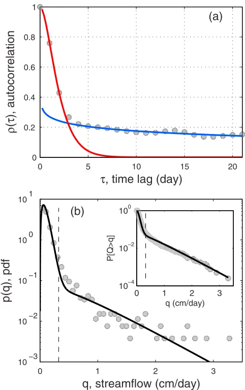
Figure 2. Statistical properties of daily streamflow of a watershed in Georgia, USA: (a) autocorrelation and (b) prob-ability density function (pdf ) and exceedance probprob-ability (inset). The dots and lines represents the empirical and mod-eled patterns, respectively; in Figure 2a, the red line repre-sents the model result associated with the high‐flow regime, and the blue line represents the low‐flow regime. The vertical dashed line represents the thresholdq*. The significant scat-ter in the empirical frequencies in the high‐flow range likely stems from the reduced statistical reliability inherent in sam-pling these infrequent events.

intermittent streams. Finally, as the results suggest, we expect the method’s performance to be limited in addressing extreme streamflows. This limitation likely stems from the fact extreme daily rainfall events are not well captured by the exponential distribution.

[27] Let us emphasize here that the key purpose of this

paper is to introduce and demonstrate some applications of this method. Accordingly, the goal of some of the discussion in the preceding section was not meant to be conclusive but rather to offer some ideas regarding the potential analyses accompanying the method. In this light, we now briefly dis-cuss some possible avenues of research linking the model parameters to relevant physical processes.

[28] The high‐flow response is likely related to the

tradi-tional instantaneous unit hydrograph, which can be derived from the drainage structure and the width function of the watershed [see, e.g., Rodriguez‐Iturbe and Valdes, 1979; Rodriguez‐Iturbe and Rinaldo, 1997]. As such, it may be possible to estimateaHandbHdirectly from the width func-tion of the watershed, thereby more directly linking its geo-morphological structure to the autocorrelation function.

[29] The low_‐flow response, which is related to

subsur-face flows and characterized byaLand bL, depends on the geology, subsurface architecture, and topography of the watershed. As is true for parameters characterizing many sub-surface processes, estimatingaLand bL directly from these underground features is difficult, especially for routine anal-ysis. The capability to estimate them from the more readily available autocorrelation function is indeed one of the key contributions of this method. Here, a potential future research direction is to apply the method to many watersheds with different geological settings and under different climates and examine the relationships between bL and these environ-mental factors.

[30] It is worth noting that some values ofaLandaHin the case studies significantly differ from 1, which corresponds to the exponential‐decay response in models based on the linear reservoir concept [e.g.,Botter et al., 2007a].This result lends support to the more recent research, which attempts to char-acterize streamflow as nonlinear functions of water storage in the system (i.e., nonlinear reservoirs) [e.g.,Kirchner, 2009; Botter et al., 2009].

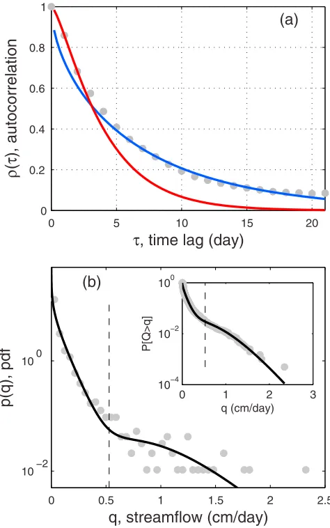
Figure 4. Statistical properties of daily streamflow of a watershed in Texas, USA: (a) autocorrelation and (b) proba-bility density function (pdf ) and exceedance probaproba-bility (inset). The legend is the same as in Figure 2.

Figure 5. Statistical properties of daily streamflow of a watershed in California, USA: (a) autocorrelation and (b) probability density function (pdf ) and exceedance prob-ability (inset). The legend is the same as in Figure 2.

MUNEEPEERAKUL ET AL.: GAMMA PULSE STREAMFLOW ANALYSIS W11546 W11546

[31] In this method, the frequencies and contributions to

the overall streamflow of the two flow regimes are rep-resented byfL,l′Land l′H. They result from the interplay between the rainfall stochasticity and soil moisture dynamics. This calls for the type of analysis presented in the studies byLaio et al. [2001] andRodriguez‐Iturbe and Porporato [2004]. Indeed, Botter et al. [2007a] have performed such analysis with the focus on the slow component. One aspect of the soil moisture dynamics that is particularly important to the high‐flow regime is the antecedent condition when a new rainfall event arrives. The antecedent condition directly controls D, which determines both the frequency and the amount of excess rainfall that eventually becomes stream-flow. Incorporating this dynamical aspect of D poses a challenge for future research [see alsoVan de Griend et al., 2002; Botter et al., 2007a]. Importantly, once the relative contributions of the two flow regimes can be made explicit functions of rainfall stochasticity, we will be in a much better position to predict changes in streamflow patterns under changing environments such as those resulting from global climate change.

[32] The present method has been developed in an

application‐oriented manner. While it offers an effective practical tool to analyze and gain understanding from empir-ical streamflow data, we are currently pursuing a more mathematically rigorous and theoretically satisfying devel-opment of the same concepts. This will enable us to derive other important properties of streamflow, such as crossing properties, which are directly relevant to flooding and water inputs into riparian zones and wetlands.

[33] Acknowledgments. R. M. and I. R.‐I. gratefully acknowledge the support from the James S. McDonnell Foundation through a grant for Studying Complex Systems (220020138). S. A. acknowledges the support from Princeton Environmental Institute.

References

Beven, K. J. (2001),Rainfall‐Runoff Modelling: The Primer, John Wiley, New York.

Botter, G., A. Porporato, I. Rodriguez‐Iturbe, and A. Rinaldo (2007a), Basin‐scale soil moisture dynamics and the probabilistic characterization of carrier hydrological flows: Slow, leaching‐prone components of the hydrologic response,Water Resour. Res.,43, W02417, doi:10.1029/ 2006WR005043.

Botter, G., F. Peratoner, A. Porporato, I. Rodriguez‐Iturbe, and A. Rinaldo (2007b), Signatures of large‐scale soil moisture dynamics on streamflow statistics across U.S. climate regimes,Water Resour. Res.,43, W11413, doi:10.1029/2007WR006162.

Botter, G., S. Sanardo, A. Porporato, I. Rodriguez‐Iturbe, and A. Rinaldo (2008), Ecohydrological model of flow duration curves and annual min-ima,Water Resour. Res.,44, W08418, doi:10.1029/2008WR006814. Botter, G., A. Porporato, I. Rodriguez‐Iturbe, and A. Rinaldo (2009),

Non-linear storage‐discharge relations and catchment streamflow regimes,

Water Resour. Res.,45, W10427, doi:10.1029/2008WR007658. Bras, R. L., and I. Rodriguez‐Iturbe (1993),Random Functions and

Hydrology, Dover, New York.

Camporeale, C., and L. Ridolfi (2006), Riparian vegetation distribution induced by river flow variability: A stochastic approach,Water Resour. Res.,42, W10415, doi:10.1029/2006WR004933.

Claps, P., A. Giordano, and F. Laio (2005), Advances in shot noise mod-eling of daily streamflows,Adv. Water Resour.,28, 992–1000, doi:10.1016/j.advwatres.2005.03.008.

Cox, D. R., and V. Isham (1980),Point Processes, Chapman Hall, Boca Raton, Fla.

Farmer, D., M. Sivapalan, and C. Jothityangkoon (2003), Climate, soil, and vegetation controls upon the variability of water balance in temperate and semiarid landscapes: Downward approach to water balance analysis,

Water Resour. Res.,39(2), 1035, doi:10.1029/2001WR000328. Kirchner, J. W. (2006), Getting the right answers for the right reasons:

Linking measurements, analyses, and models to advance the science of hydrology,Water Resour. Res., 42, W03S04, doi:10.1029/ 2005WR004362.

Kirchner, J. W. (2009), Catchments as simple dynamical systems: Catch-ment characterization, rainfall‐runoff modeling, and doing hydrology b a c k w a r d , W a t e r R e s o u r . R e s ., 4 5, W 0 2 4 2 9 , d o i : 1 0 . 1 0 2 9 / 2008WR006912.

Laio, F., A. Porporato, L. Ridolfi, and I. Rodriguez‐Iturbe (2001), Plant in water‐controlled ecosystems: Active role in hydrologic processes and response to water stress—II,Adv. Water Resour.,24, 707–723. Muneepeerakul, R., A. Rinaldo, and I. Rodriguez‐Iturbe (2007), Effects of

river flow scaling properties on riparian width and vegetation biomass,

Water Resour. Res.,43, W12406, doi:10.1029/2007WR006100. Nash, J. E. (1957), The form of the instantaneous unit hydrograph,IASH

Publ.,45, 114–121.

Perona, P., C. Camporeale, E. Perucca, M. Savina, P. Molnar, P. Burlando, and L. Ridolfi (2009), Modelling river and riparian vegetation interac-tions and related importance for sustainable ecosystem management,

Aquat. Sci.,71(3), doi:10.1007/s00027-009-9215-1.

Rodriguez‐Iturbe, I., and A. Porporato (2004),Ecohydrology of Water‐

Controlled Ecosystems: Soil Moisture and Plant Dynamics, Cambridge Univ. Press, Cambridge, U. K.

Rodriguez‐Iturbe, I., and A. Rinaldo (1997),Fractal River Basins: Chance and Self‐Organization, Cambridge Univ. Press, Cambridge, U. K.

Rodriguez‐Iturbe, I., and J. B. Valdes (1979), The geomorphologic struc-ture of hydrologic response,Water Resour. Res.,15(6), 1409–1420, doi:10.1029/WR015i006p01409.

Rodriguez‐Iturbe, I., V. K. Gupta, and E. Waywire (1984), Scale considera-tions in the modeling of temporal rainfall,Water Resour. Res.,20(11), 1611–1619, doi:10.1029/WR020i011p01611.

Rodriguez‐Iturbe, I., D. R. Cox, and V. Isham (1987), Some models for rainfall based on stochastic point processes,Proc. R. Soc. London, Ser. A,410(1839), 269–288.

Rodriguez‐Iturbe, I., D. R. Cox, and V. Isham (1988), A point process model for rainfall: Further developments,Proc. R. Soc. London, Ser. A,

417(1853), 283–298.

Rodriguez‐Iturbe, I., A. Porporato, L. Ridolfi, V. Isham, and D. R. Cox (1999), Probabilistic modelling of water balance at a point: The role of climate, soil and vegetation,Proc. Roy. Soc. London, Ser. A,455, 3789–3805.

Van de Griend, A. A., J. J. De Vries, and E. Seyhan (2002), Ground-water discharge from areas with a variable specific drainage resistance,

J. Hydrol.,259, 203–220.

Weiss, G. (1977), Shot noise models for the generation of synthetic stream-flow data, Water Resour. Res., 13(1), 101–108, doi:10.1029/ WR013i001p00101.

Xu, Z. X., G. A. Schultz, and A. Schumann (2002), A conceptually based stochastic point process model for daily streamflow generation,Hydrol. Process.,16, 3003–3017, doi:10.1002/hyp.1085.

S. Azaele, Institute of Integrative and Comparative Biology, University of Leeds, Miall Bldg., Leeds LS2 9JT, UK.

G. Botter, Dipartimento di Ingegneria Idraulica, Marittima, Ambientale e Geotecnica, Università di Padova, via Loredan 20, I‐35131, Padua, Italy.

R. Muneepeerakul, School of Sustainability, Arizona State University, PO Box 875502, Tempe, AZ 85287‐5502, USA. (rachata.muneepeerakul@ asu.edu)

I. Rodriguez‐Iturbe, Department of Civil and Environmental Engineering, Princeton University, E‐Quad, Princeton, NJ 08544, USA. A. Rinaldo, Laboratory of Ecohydrology, Faculté ENAC, Ecole Polytechnique Federale, Lausanne, CH‐1015, Switzerland.

MUNEEPEERAKUL ET AL.: GAMMA PULSE STREAMFLOW ANALYSIS W11546 W11546