Published By:
Abstract, This work deals with the analytical solution of the rise temperature history on the back face of the unfired clay bricks related to the theoretical model of flash method, was calculated using Duhamel theorem. The local sensitivity analysis of the obtained solution shown that the sensitivity coefficients related to the thermal diffusivity and the adiabatic limit temperature meets the beck criterion for low time range, so these tow parameters can be simultaneously estimated with a good accuracy in this time range. Due to the slow convergence of the analytical solution in short times, the procedure for estimating the thermophysical properties is relatively slow. The theoretical analytical solution has therefore been replaced by an equivalent solution whose convergence speed was improved using the Wynn Epsilon method. The apparent thermal diffusivity and the adiabatic limit temperature of samples were then estimated by fitting measured rise temperature with the equivalent analytical solution. It is interesting to note the good agreement between the theoretical model with predicted values of parameters and the experimental data.
Keywords : Thermophysical properties, The flash method, Analytical solution; Numerical solution; Earthen materials.
I. INTRODUCTION
At the international level, the building sector is one of the main energy consumers with around 28% of final energy consumption [1] and contributes around a third of CO2 emissions [1]. As a result, reducing energy costs in this sector is a major challenge to energy strategies in many countries.
In the following, we present a brief survey of studies published in recent years concerning the measurement of the thermophysical properties of building materials, with a special attention put on methods for the thermal diffusivity identification from flash method. Chihab et al [2] investigated the adiabatic limit temperature and the thermal diffusivity of unfired clay brick by using a numerical inverse estimation. In this study a global minimization algorithm is used and the theoretical model of flash method is calculated using a semi analytical solution. In the work of Michele Dondi et al [3] the thermal conductivity of clay brick was determined and correlated with the compositional, physical and microstructural properties of the raw materials. El Azhary et al [4] tried to valorize
Revised Manuscript Received on September 07, 2019. * Correspondence Author
Yassine Chihab*, Mohammed V University in Rabat, Materials, Energy and Acoustics TEAM, Morocco.
Mohammed Garoum, Mohammed V University in Rabat, Materials, Energy and Acoustics TEAM, Morocco
Najma Laaroussi, Mohammed V University in Rabat, Materials, Energy and Acoustics TEAM, Morocco
agricultural residues such as wheat straw in the manufacture of construction materials. In particular they showed that the addition of straw improve significantly the thermal properties of unfired clay brick. Stefania Liuzzi et al [5]-[6] examined the improvement of the thermal properties of earthen brick mixed with olive fibers. Chihab et al [7] studied the effect of clay consistency on the thermal properties of the composite material clay_straw.
The majority of studies concerning the thermal diffusivity estimation are investigated using a numerical theoretical solution. In this research, The thermal diffusivity is estimated by solving analytically the transient heat conduction equation using Duhamel theorem under time-dependent convection boundary conditions of flash model.
The present work deals with the study of thermophysical properties of raw brick walls made from earth collected in three different sites in Morocco.
II. EXPERIMENTALAPPROACH
A. Samples preparation
Three different raw clays extracted from three Moroccan sites (clay of Marrakech (CM), clay of Tamansourt (CT) and clay of Essaouira (CE)) were studied.
The Atterberg limit test and particle size analysis were carried out to determine the geotechnical and the physical properties of the raw material. Particle size distribution was determined using a sieving test according to standard NF P 94-056[8]. Figure 3 shows the grain size distribution for the clay used. Consistency limits were determined using a standard method NF P94-052.1[9] and NF P94-051[9] for measuring liquid and plastic limits, respectively. Table 1 illustrates the Atterberg limits obtained for raw clay. Plasticity index was also reported on this table.
Table-I: The Atterberg limits of the three raw clays used
sample
Atterberg Limits Liquidity
Limit(%)
Plasticity Limit(%)
Plasticity Index(%)
Clay (CM) 37 23 14
Clay (CT) 65 25 40
Clay (CE) 46 26 20
The mineralogy of each clay was characterized using X-Ray Diffraction analysis. The results are in figure 1. The samples are generally composed
of: quatrz, calcite,
Thermophysical Characterization of Earthen
Materials Using the Flash Method
dolomite and clay minerals (Kaolinite, Illite, and Vermiculite).
[image:2.595.313.547.75.175.2].
Fig. 1. X-Ray Diffraction of raw clay (a: CM),(b: CT),(c: CE)
Three samples were then prepared ( Fig 2). The water to clay ratio was kept equal to 28%.The samples were then dried in an oven at 70°C during three days and packed in plastic films to avoid any moisture contamination.
[image:2.595.50.276.105.365.2]
Fig. 2.Studied samples (a) CT, (b) CE, (c) CM
[image:2.595.309.468.301.490.2]
Fig. 3.Grain size curves of the three clays
III. THERMALDIFFUSIVTY ESTIMATION BY
THEFLASHMETHOD
This method is mainly used to estimate the thermal diffusivity of materials. Its basic principle is described in the Figure 4. The front face of the sample is exposed to a strong heat pulse and the variation of the rise temperature with time is measured at the rear face. Temperature with time is
[image:2.595.71.271.469.513.2]measured at the rear face using a thermocouple type K.
Fig. 4.Schematic of the flash method A. Mathematical model
In order to have one dimension heat conduction across the sample, its lateral sides were isolated. We assume that the absorbed energy at the front face is uniform and the initial temperature T0 is equal to the ambient one. The rise temperature T is then governed by the following system (1).
2T x ,t 1 T a t 2
x
h
T x ,t 1 .T 0 ,t g t x 0
x
h T x ,t 2 .T e ,t
x e x
T x ,0 0 (1)
.
d d
d 0
0 g
t
t Q f
1
, t . t
With f (t)
0 , t t
t.
[image:2.595.65.277.544.665.2]Published By:
t 0T x ,t R x ,t , d
t (2)
Where R (x, t, μ) is the solution of the auxiliary system (3) and is a parameter.
2 2 1 x 0 2 x eR x, t, 1
R x, t,
.
a t
x
R x, t, h
.R 0, t, g . x
R x, t, h
.R e, t, . x
R x,0, 0
(3) The system (3) can be reduced to a problem with
homogeneous boundary conditions by assuming that R(x, t, μ) has the following from:
R x, t, U x, t, M x, t, (4) Where U(x, t, μ) is an arbitrary function satisfying the
two boundary conditions (5):
1 x 0 2 x eU x, t, h
.U 0, t, g .
x
U x, t, h
.U e, t, . x (5)
We take for U(x,t,μ) the following form :
x
xU x, t, A t . 1 B t .
e e
(6)
A and B can be calculated using the boundary conditions (5)
For x=0:
22 1 2 1
2 1 2 1
e.h
(1 ).e.g
A
e.h e.h e.h e.h
.
e.g
B .
e.h e.h e.h e.h
.
We have :
2 2
R x, t, 1
R x, t,
. a t x
(7)
Replacing Eq. (4) in (7) conduct to :
2 2
2 2
U x,
M x, t,
1
1
U x,
M x, t,
.
.
a
t
a
t
x
x
With :
2 2 U x, 0 x U x, 0 t
2 2M x, t, 1
M x, t,
. a t x (8) Then the function M(x, t, μ) must be the solution of the
problem:
2 2 1 x 0 2 x eM x, t, 1
M x, t,
.
a t
x
M x, t, h
.M 0, t, .
x
M x, t, h
.M e, t, .
x
M x, 0, U x,
(9) Resolution of system (9) by the Variable Separation
Method:
M x ,t , A x , C t (10)
Replacing Eq.(10) in the system (9) leads to the following equations:
2A x,
2 1
C t
C t . A x, .
a t x
2 2 2 C t1 A x, 1
f .
A x, x a.C t t
f is a constant because the two functions A(x,μ) and C(t) depend on one of x, μ and the other on t.
2 2 f .a.t 2 2 2 C ta.f C t 0 t
C t c.e
A x,
f .A x, 0 x
A x, a.Cos f .x b.Sin f .x
The superposition principle allows to write the general solution of equation (8) in the
n n n 0
M x ,t , C t A x ,
With :
n n n n n
A x, a .Cos f .x b .Sin f .x
(11) For x=0:
n 1 1
x 0 n n n n
A x h h
.A 0 b f a
x n n n 1
a
f
b
h
(12) elacing Eq. (A.12) in (A.11) conduct to :
1
n n n n
n
h
A x a Cos f .x .Sin f .x
.f
(13)
For x=e
n 2
x e n
A x h
.A e x
1 2 n n2 1 2
n
h h
f Tan f .e
h h f (14) an can be calculated by using orthogonality properties of
the normalized eigenfunctions An(x) Eq.(15):
e
n m
0
0 si n m.
A x, A x, dx
1 si n m.
(15)
2e
2 1
n n n
n 0
h
a Cos f .x .Sin f .x dx 1 .f
n 2 e 1 n n n 0 1 a hCos f .x .Sin f .x dx .f
We obtain:
n 1 n 2n n n
n
n 1 1 n
.f h a
Sin 2f .e .f Sin 2f .e
e e
Sin f .e
2 4f h h 2 4f
(16)
Using Eq .(12) bn can be written as :
n
2
n n n
n
n 1 1 n
1 b
Sin 2f .e .f Sin 2f .e
e e
Sin f .e
2 4f h h 2 4f
(17)
cn can be calculated using the initial condition :
n n n 0
M x ,0 , c A x , at t 0
Assuming the uniform convergence and the orthogonality of the normalized eigenfunction An(x, µ)
n
n
n
n
n 0
A
x ,
M x ,0 ,
A
x ,
c
A
x ,
e e
n n n n
n 0
0 0
A x , M x ,0 , dx A x , c A x ,
e
n n
0
c A x , M x ,0 , dx
(18)
We develop the calculation of integral in Eq.(18) we obtain :
n n n n
c R L K (19) With :
2n n n
n n n
2 1 2 1 n n n
2
n
n n 2 n 2
2 1 2 1 n n n
2 n
2 1
e.h
(1 ).e.g
a b b
R Sin f .e Cos f .e .
e.h e.h e.h e.h f f f
.
e.h
( ).g Cos f .e
e 1
L .a Sin f .e .
e.h e.h e.h e.h f f f
.
e.h
( ).g
K
e.h e.h e.
n
nn 2
2 1 n n
e.Cos f .e Sin f .e
.b .
h e.h f f
.
Assuming a square shape of the heat pulse g(t), the temperature on the back side of the sample is finally given by the following new expression :
. . . . . .. os . . in . .
. . . . . 2 2 n d n 2 ma i 2 d th n 1
f a t t f a t
i 1 2 2 n 4 2 n n n n n e T 2 b t a K T b C f e
e f f e D f e
e e f S f e e
(20)
WWWWWW
WWWWW
i 1 i 2 i 2 i 1 i 1 i
2 2 2 2
2 2
2
i 1 i 2 i 1 i 2
b b b b b b
b b b b
k D
e is the thickness of the sample, 0 ma
Q T
ce
is the adiabatic limit temperature, c is the specific heat , ρ is the density, 1
i1 h e
b
i2 2 h e
, b
Published By:
Where the eigenvalues fn are solutions of the
transcendental equation:
n i1 i2
n 2
n i1 i2
e.f b b
Tan f .e
e.f b b
B. Local sensitivity analysis
Four unknown parameters are involved in the theoretical model namely Tma, a, bi1 and bi2.
The four parameters will be estimated simultaneously from measured and theoretical model of flash method.
The theoretical involves four unknown parameters namely Tma, a, bi1 and bi2. These parameters will be estimated. However, the analysis of their sensitivities coefficients must be carried out before, in order to identify which parameters can be simultaneously predicted with a reasonable accuracy. The main condition to estimate simultaneously all parameters is that their sensibility coefficients must be different from zero and linearly independent ( Beck criteria[11]). Moreover the central idea, beyond the sensitivity analysis, is to determine the time interval in which the model is very sensitive to a small change of the parameter to be inferred.
For a given parameter the relative coefficients of sensitivity is defined as:
With 1, 2, 3, 4
k k h k
T
k
Where ηk is the unknown parameters (η1=a, η2=Tma ,η3=bi1,η4=bi2). All of the above derivatives was performed analytically using Mathematica 11.3 language.
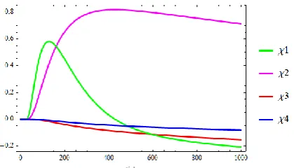
[image:5.595.57.267.515.635.2]Figure 5 shows an example of the variation of the relative coefficients of sensitivity with time.
Fig. 5. Relative coefficients sensitivity curves (bi1=0.2 bi2=0.1 e=0.01m a=10-7m2/s Tma=1°C) We can see that the model is more sensitive to the change in a and Tma . Their sensitivity coefficients meets the beck criteria[11] for low time range (t<350s). So a and Tma can be simultaneously determined with a good accuracy in this time range. We also notice that the model is very weakly sensitive to bi1 and bi2.Their sensitivity coefficients are both very small and correlated over most of the time interval. As a result, these tow later parameters cannot be estimated with a good accuracy.
The analytical series solution converges very slowly especially at low times making the estimation procedure of parameters very time consuming. To improve the convergence, the original solution was transformed using the speeding technique of Wynn's Epsilon [12].
The method provides an efficient algorithm for implementing transformations of the form:
1 21 2 1
n n n
n
n n n
S S S T S
S S S
(21) Where :
0
n
n k
k
S a
(22) is the partial sum of a sequence
ak k
that is useful for improving series convergence.
With :
2 2 2
2
. . 1
2 2
4 2
.
2 . .
.
. os . . in
.
. . .
. . .
k d k
ma i d
f a t t f a t k k
k k
k i
k k
e f a
f e D f e
e e T
b t a
K
f b
C f e S f e e e
(23)
The basic definitions of the Epsilon algorithm are given as follows:
1 0
0
n n
n
S
(24)For j = 1,2,. . . then we calculate the new estimates by:
1
1 1 1
1
,
n n
k k n n
k k
k n
N
(25)
Fig. 6. Comparison between the analytical solution with and without convergence acceleration (bi1=0.0007
[image:6.595.45.276.419.628.2]bi2=0.0007 e=0.02m a=8×10⁻⁷m2/s Tma=1.3°C)
Fig. 7.comparison between the analytical solution with and without convergence acceleration (bi1=1 bi2=1.5
e=0.02m a=3×10⁻⁷m2/s Tma=1.3°C)
C. Comparison with solution derived from the Laplace transform technique
The validation of the analytical solution has been carried out with a semi analytical solution using numerical inversion of Laplace transform.
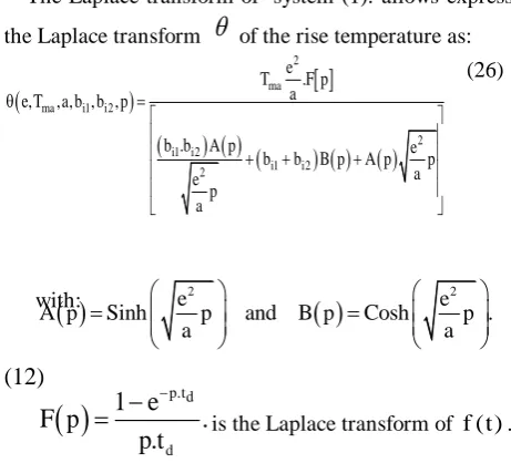
The Laplace transform of system (1). allows expressing the Laplace transform
of the rise temperature as:
ma i1 i2
2 ma
2 i1 i2
i1 i2 2
e T .F p
a
b .b A p e
b b B p A p e,T ,a,b ,
p e
b ,p
a p
a
(26)
(12)
with:
e2
e2A p Sinh p and B p Cosh p .
a a
p.tdd
1 e
F p
.
p.t
is the Laplace transform of f (t) .Gaver -Stehfest’s algorithm [13] approximates the solution in the reel space using the following equation :
Fig. 8.Comparison between the analytical and numerical solutions (bi1=3.34 bi2=3 e=0.02m
a=5×10⁻⁷m2/s Tma=1.2°C)
1 2 2
1
1
( , , , , , ) ln(2) . , , , , ,ln(2). n
th ma i i j th ma i i
j
T e T a b b t V e a b j
t T b t
(27) The coefficients Vj are given by the relation :( , ) ( 1)
2 2
( ) 2
1 2
( ) (2 )!
( 1)
( )!( )!( )!(2 1)!
2
n n
Min j n
j j
j k
k k
V
n
k k i k k
(28)The figures 8 and 9 show the curves given by the new analytical solution and the solution obtained by numerical inversion using Gaver -Stehfest method. As we can see there is a good agreement between the two solutions.
D. Local Minimization Procedure
The optimal values of the Tma, a bi1 and bi2 are sought so as to minimize the quadratic distance M between Tth and the experimental thermogram Eq.(29)
N 2ma i1 i2 exp j th ma i1 i2 j
( j 1)
e,T ,a,b ,b T (t ) T (e,T ,a,b ,b ,t )
(29)A local minimization can be used to estimate the unknown parameters. The Principal Axis Algorithm of Brent) [14] was then chosen. It is derivative-free algorithm and it needs two distinct starting conditions for each parameters.
For the thermal diffusivity, the starting conditions are calculated using the Parker’s formula (Eq.30). [15]
Par ker
Par kera
a
,1.1 a
While the starting conditions of the adiabatic limit temperature (Tma) are calculated by
ma max ex max ex
T
T
,1.1 T
Where
2
Par ker
1 / 2 e a 0.1388
t (30)
e is the sample thickness and t1/2 is the time up to reaching half of the maximum Tmaxex of the experimental
thermogramTex on the rear face.
It is worth mentioning that for a model with heat loss at rear and front faces of sample (bi1≠0 and bi2≠0) we have
ma max imum
T
T
[image:6.595.59.259.681.796.2]Published By:
discussed in order to compare a local minimization (Principal axis method of Brent algorithm) [14] with a global minimization (Nelder Mead ) [16] used in previous work [2].
IV. RESULTANDDISCUSSION
It is noticed that the thermal diffusivity and the adiabatic limit temperature in table II were estimated using the analytical solution combined with Wynn's Epsilon method to calculate the theoretical model of flash method and a local minimization procedure (Principal axis method of Brent).
The experiment has been repeated three times on the same sample for flash method and hot steady plate in order to determine the experimental relative measurement deviation, and then to take the mean value from the three experiments as result of the thermal properties characterization.
The relative measurement deviation is defined as:
m
m
E E
100 E
WhereEm is the average value of the thermal properties
and Eis the estimated value of the thermal properties. The deviation gives quite acceptable results. (maximum deviation of about 2% for the thermal diffusivity). The apparent densities are easily calculated knowing the dimensions and masses of the dry samples. As evident from Table 1 that the clay (CM) has the highest density of 1890.256kg/m3.While,the clay (CE) has the lowest ones.
According to the results of Table II, it is noticed that the adiabatic limit temperature increases with the decrease of density. In addition, the clay (CM) has the lowest value of the adiabatic limit temperature which means that it has the highest value of volumetric capacity (ρ.c).
Table- II: The thermal diffusivity and the adiabatic limit temperature of the two types of unfired clay brick Sample Test
Estimated diffusivity a×10-7[m2.s-1]
Measurement deviation (%)
Estimated Tma
[°C] ρ [kg/m3]
Clay (CT)
1 3.290 1.300 1.036
1616.83
2 3.261 0.300 1.004
3 3.194 1.720 0.989
Mean
value 3.250 _ 1.009
Clay (CE)
1 3.013 0.060 1.049
1616.16
2 3.020 0.160 1.041
3 3.014 0.030 1.082
Mean
value 3.015 _ 1.060
Clay (CM)
1 3.641 1.470 0.970
1890.25
2 3.618 0.800 0.913
3 3.506 2.000 0.964
Mean
value 3.588 _ 0.949
Table- III: Comparison between local and global minimization algorithms Sample Test
Local minimization Present work a×10-7[m2.s-1]
Gocal minimization
[2] a×10-7[m2.s-1]
Deviation [%]
Local minimization Present work
Tma [°C]
Gocal minimization
[2] Tma [°C]
Deviation [%]
Clay (CT)
1 3.290 3.284 0.18 1.036 1.034 0.19
2 3.261 3.264 0.09 1.004 1.000 0.39
3 3.194 3.197 0.09 0.989 0.985 0.4
Clay (CE)
1 3.013 3.005 0.26 1.049 1.0468 0.2
2 3.020 3.009 0.36 1.041 1.041 0
3 3.014 3.003 0.37 1.081 1.081 0
Clay (CM)
1 3.641 3.659 0.49 0.970 0.964 0.62
2 3.618 3.625 0.19 0.913 0.908 0.5
Table III presents a comparison between local and global minimization algorithms to estimate the thermal diffusivity and the adiabatic limit temperature of the two types of unfired clay bricks. It can be readily shown in table III that the two algorithms give similar results but the global minimization algorithm converge more slowly. Regarding the computational efficiency as manifested by the needed CPU times of the two algorithms in table IV we can see that (CPU) time consumed is very long for the global minimization algorithm (CPU t=40.177s) compared with CPU time consumed for the local minimization algorithm (only CPU t=1.737s). We can conclude that the local minimization procedure is more interesting for our problem (flash method) because it is can give a similar results as the global minimization and it is can be converge very quickly.
Table-IV: The computational efficiency of several estimation procedures of flash method Sample Test
Local minimization Present work CPU time(sec)
Global minimization
[2] CPU time(sec) Clay
(CT)
1 1.825 39.561
2 1.716 38.129
3 1.872 38.501
Clay (CE)
1 2.010 38.137
2 1.669 39.855
3 1.622 41.820
Clay (CM)
1 1.684 41.917
2 1.622 42.120
3 1.620 41.558
_ Mean
value 1.737 40.177
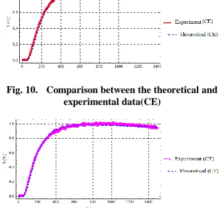
The estimated parameters are then injected into the theoretical model in order to compare it with the experimental data. Figures 9,10 and 11 present the predicted and measured temperature at rear face for the three types of unfired clay brick. It is interesting to note the good agreement between the theoretical model with predicted values of parameters and experimental data.
Fig. 9.Comparison between the theoretical and experimental data(CM)
[image:8.595.72.266.265.465.2]Fig. 10. Comparison between the theoretical and experimental data(CE)
Fig. 11. Comparison between the theoretical and experimental data(CT)
V. CONCLUSION
This work presents theoretical and experimental investigations to evaluate the thermophysical properties of earthen walls mad from three types of unfired clay bricks. From the results, it can be noted the conclusions below : 1) .An analytical solution is used to estimate the thermal diffusivity and the adiabatic limit temperature.
2). Whynn's Epsilon method improves significantly the computational efficiency and the numerical integration speed of the analytical solution of flash model with almost similar accuracy.
3). A local minimization is more interesting as a global minimization to estimate a and Tma from the flash method. 4). Increases in density causes an increase in the thermal diffusivity of samples
ACKNOWLEDGMENT
The present research study is part of the λ@DB project which aims to develop a national database of the thermophysical properties of the main local building materials in Morocco, supported by the German International Cooperation (GIZ).
REFERENCES
1. Moroccan Agency for the Energy Efficiency (AMEE).Règlement Thermique de Construction au Maroc. 2014. www.amee.ma.
2. Chihab, Yassine, et al. "Numerical inverse estimation of the thermal diffusivity and the adiabatic limit temperature of three types of unfired clay bricks using flash method and global minimization algorithm." IOP Conference Series: Materials Science and Engineering. Vol. 446. No. 1. IOP Publishing, 2018.
3. Dondi, M., Mazzanti, F., Principi, P., Raimondo, M., & Zanarini, G.(2004).Thermal conductivity of clay bricks. Journal of materials in civil engineering, 16(1), 8-14.
[image:8.595.58.279.568.660.2]Published By:
Author-1 Photo
Author-2 Photo
Author-3 Photo
Material Clay-straw. Energy Procedia. 141. 160-164.
5. Liuzzi, S., Rubino, C., & Stefanizzi, P. (2017). Use of clay and olive pruning waste for building materials with high hygrothermal performances. Energy Procedia, 126, 234-241.
6. Liuzzi, S., Rubino, C., Stefanizzi, P., Petrella, A., Boghetich, A., Casavola, C., & Pappalettera, G. (2018). Hygrothermal properties of clayey plasters with olive fibers. Construction and Building Materials, 158, 24-32. 7. Chihab, Yassine, et al. "The Effect of Clay Consistency on the
Thermophysical Properties of Composite Material Clay-straw." 2018 6th International Renewable and Sustainable Energy Conference (IRSEC). IEEE, 2019.
8. AFNOR, N. (1995). 94-056: Sols: reconnaissance et essais. Analyse granulométrique: méthode par tamisage à sec après lavage. Normalisation Française.
9. AFNOR. (1993). NF P94-051 Sols: reconnaissance et essais; Détermination des limites d’Atterberg–Limite de liquidité à la coupelle-Limite de plasticité au rouleau [Soil: Investigation and testing. Determination of Atterberg’s limits. Liquid limit test using cassa grande apparatus. Plastic limit test on rolled thread].
10.Laaroussi, N., et al. "Measurement of thermal properties of brick materials based on clay mixtures." Construction and Building Materials 70 (2014): 351-361.
11.Beck.J.V. Parameters estimation in engineering and science. Wiley& sons. USA. 1989.
12.P. Wynn The epsilon algorithm and operational formulas of numerical analysis Math. Comp., 15 (1961), pp. 151-158.
13.Stehfest. Numerical inversion of Laplace transforms.Communications of the Association for Computing Machinery. 1970.
14.Brent, Richard P. Algorithms for minimization without derivatives. Courier Corporation, 2013
15.Parker, W. J., et al. "Flash method of determining thermal diffusivity, heat capacity, and thermal conductivity." Journal of applied physics 32.9 (1961): 1679-1684.
16.J. A. Nelder and R. Mead, A simplex method for function minimization, Computer Journal 7 (1965), 308–31
AUTHORSPROFILE
Yassine CHIHAB has an engineer's Degree in civil engineering in 2016 from Cadi Ayyad University, Marrakech. His fields of interest include materials and building energy efficiency, thermal characterization, simulation of thermophysical properties of building and construction materials, numerical inverse estimation based gradient and global algorithms.
Mohammed GAROUM is currently Professor at the Higher School of Technology of Salé (ESTS), University Mohammed V of Rabat, Morocco since 1995. In 1991 he received his first PH.D in acoustics from the Ecole Central de Lyon France. In 1997 his was awarded his second State Doctorate in Photoconductivity of semiconductor from the Institute of Sciences of Engineering and Scientific Development at Claude Bernard University Lyon I and Faculty of Sciences of Cadi Ayyad University, Marrakech. Prof M.GAROUM is the author and co-author of more than 50 scientific publications and communications mainly related to materials and building energy efficiency, experimental characterization and simulation of thermophysical and acoustical properties of building and construction materials, numerical inverse estimation of thermal and acoustical parameters based gradient and global algorithms.