HYD Verifications Using Numerical Methods

This is a repository copy of HYD Verifications Using Numerical Methods. White Rose Research Online URL for this paper:

http://eprints.whiterose.ac.uk/109832/ Version: Accepted Version

Article:

Katsigiannis, G, Ferreira, P and Fuentes, R orcid.org/0000-0001-8617-7381 (2018) HYD Verifications Using Numerical Methods. Georisk, 12 (1). pp. 45-59. ISSN 1749-9526 https://doi.org/10.1080/17499518.2016.1269182

© 2017 Informa UK Limited, trading as Taylor & Francis Group. This is an Accepted Manuscript of an article published by Taylor & Francis in Georisk on 18 January 2017, available online: http://dx.doi.org/10.1080/17499518.2016.1269182

[email protected] https://eprints.whiterose.ac.uk/

Reuse

Items deposited in White Rose Research Online are protected by copyright, with all rights reserved unless indicated otherwise. They may be downloaded and/or printed for private study, or other acts as permitted by national copyright laws. The publisher or other rights holders may allow further reproduction and re-use of the full text version. This is indicated by the licence information on the White Rose Research Online record for the item.

Takedown

If you consider content in White Rose Research Online to be in breach of UK law, please notify us by

HYD Verifications Using Numerical Methods

Georgios Katsigiannis

Civil, Environmental and Geomatic Engineering Department, University College

London, London, United Kingdom

[email protected]

00447543621448

Pedro Ferreira

Civil, Environmental and Geomatic Engineering Department, University College

London, London, United Kingdom

[email protected]

Raul Fuentes

School of Civil Engineering, University of Leeds, Leeds, United Kingdom

HYD Verifications Using Numerical Methods

HYD, as described in Eurocode 7, is related to the upward flow of water through

the soil towards a free surface, such as in front of a retaining wall or in the base

of an excavation. The HYD verification, using numerical analysis, can be

performed with two different approaches. The first approach is the conventional

soil block approach where safety may be checked by calculating the equilibrium

of a rectangular block of soil. The second approach is the integration point

approach where stability can be verified at every integration point in the

numerical analysis by checking that the equilibrium is satisfied for a soil column

of negligible width above each point. In this paper, the two approaches are

described and their advantages and disadvantages are discussed. Comparisons

made using benchmark geometries, extensively studied and discussed between

the members of the EC7 Evolution Group 9, on Water Pressures, illustrate that

the HYD verification using numerical methods seems very promising. Thorough

comparisons between the factors from the two approaches, allow designers to

better understand the benefits of using more advanced and robust approaches for

such stability verifications.

Keywords: HYD; hydraulic heave; Eurocode 7; water pressures

Introduction

The HYD limit state is described in Eurocode 7 (EC7) in relation to the hydraulic

heave, internal erosion and piping in the ground, caused by hydraulic gradients (BS

EN 1997-1, 2004). This covers a wide range of situations related to stability problems

caused by hydraulic gradients. McNamee (1949) made a distinction between two types

of failure relating to water pressures; piping that usually initiates locally and heave

which involves a greater soil mass.

This paper focuses on part of the EC7 definition, hydraulic heave, which is

illustrated in EC7 and shown here as Figure 1. Hydraulic heave relates to the ground

movement of a free surface caused by a vertical upward flow of water. Requirements

heave shall be checked in terms of seepage forces and buoyant weights, or in terms of

total stresses and pore-water pressures. A particular case where hydraulic heave is

relevant is in front of a retaining wall. It represents an Ultimate Limit State, potentially

resulting in sudden failure with serious consequences for people and structures.

Simpson et al. (1987) discussed problems caused by water pressures due to rising water

levels while Stroud (1987) referred to a number of situations where unforeseen water

pressures led to critical failures. Other authors have also discussed similar issues related

to safety considerations in relation to the ground water pressures (e.g. Orr 2005;

Simpson et al. 2009; Simpson 2011).

In recent years, with the advances in software and hardware, more designers are

willing to use Finite Element (FE) methods, to verify safety against hydraulic heave.

The HYD verification using FEM can be performed with two different approaches,

namely the soil block approach and the integration point approach (Evolution Group 9 -

Water Pressures, 2014).

The first approach is the conventional approach where safety may be checked by

studying the equilibrium of a rectangular block of soil. In the integration point

approach, stability can be verified at every integration point by checking the equilibrium

of a soil column of negligible width. The results are plotted as contours, rendering the

checks of whether the equilibrium is fulfilled at every integration point an easy task. In

this chapter, the two approaches are described and their advantages and disadvantages

are discussed.

Eurocode 7 requirements

Safety against failure by hydraulic heave can be verified with Equations 1 or 2 as given

by EC7 (BS EN 1997-1, 2004), where stability shall be checked in terms of seepage

Equation 1 (2.9a as referred to in BS EN1997-1, 2004) requires the design pore water

pressure, at the bottom of a relevant soil column to be less than the design total

vertical stress, . Equation 2 (2.9b as referred to in BS EN1997-1, 2004) requires

the design seepage force caused by the excess pore water pressures, to be less

than the design buoyant weight of the column,

(1)

(2)

Both equations already incorporate safety using design values (subscript d),

without further factors being shown in the requirements. The subscripts dst and stb

refer to destabilising and stabilising effects respectively.

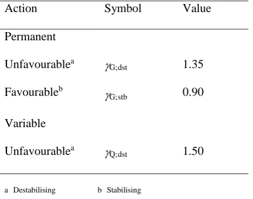
For the HYD Limit State, the typical partial factors are specified withG;dst =1.35

for permanent unfavourable actions, G;stb =0.9 for permanent favourable actions and

Q;dst =1.5 for variable unfavourable actions (see Table 1). However, EC7 does not state

precisely how these factors are to be applied in Equations 1 or 2.

Some designers apply the partial factors to the characteristic values of the

stabilising and destabilising parameters, misinterpreting the Equations 1 and 2 to mean:

(3)

(4)

Here, the subscript k refers to characteristic values of the parameters. Orr (2005)

pointed out that if the two equations are used in this way they can lead to markedly

different results for the same values of partial factors. Simpson (2012) argues that this is

a misunderstanding of the code requirement, and in particular of the concept of design

should be applied to the excess water pressures only, not to the hydrostatic component.

Orr (2005) also concluded that the partial actions factors should only be applied to the

excess pore water pressure and not the hydrostatic pressure.

EC7 notes that the load factors might not be always appropriate for ground water

pressures and allows for direct assessment of the design value or application of a safety

margin to the characteristic ground water table. Thus, by allowing three alternative

approaches, the UK National Annex leaves much of the responsibility for calculation of

the design value of water pressures with the designers (Simpson et al. 2011). Simpson

and Katsigiannis (2015) argue that factoring water pressures should generally be

avoided and favour the direct assessment of the design water pressures or the design

water table level.

Methodology

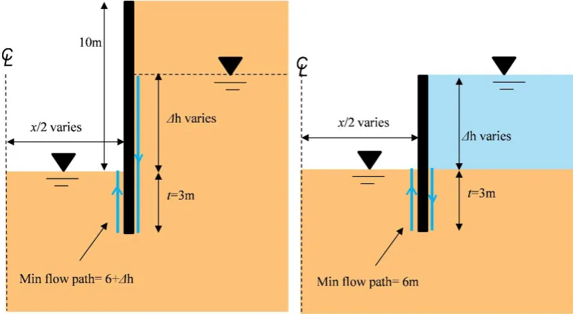
The two approaches for HYD verification using FE methods, are now illustrated for the

two simple problems presented in Figure 2, a 10m excavation and a cofferdam

geometry. The software used is Plaxis 2015.02 and the following assumptions were

made in the model:

 The wall is wished-in-place, impermeable and not allowed to deform in any

direction.

 Only half of the excavation width is modelled due to symmetry.

 The calculations are performed assuming steady state conditions while the soil is

considered fully drained; constant hydraulic head is used by specifying a fixed

water table level behind the retaining wall. In front of the wall, the water level is

defined in the formation level, at the end of the excavation.

 The side and bottom model boundaries are considered to be impermeable.

 The side model boundaries are fixed in the x direction while the bottom model boundary is fixed in both x and y directions.

 Initial stress field conditions are based on hydrostatic water pressures and K0

=1-sin ’.

 Interface elements are used between the soil and the wall with tan = 0.5tan ’,

where is the soil/wall friction angle.

The properties of the soil are given in Table 2 for an elastic-perfectly plastic soil

model such as the Mohr-Coulomb. The stiffness of the soil, which varies with depth,

has no effect on this problem. The Finite Element mesh used for the simulations, which

consists of 4332 15-node triangular elements, is given in Figure 3 for the 10m deep

excavation case. The current mesh size is adequate for this type of problem.

The Soil Block Approach

The Terzaghi’s criterion

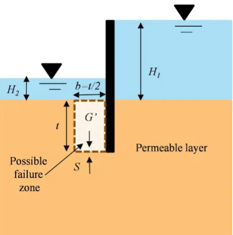
According to experimental evidence for isotropic and uniform soils, it is sufficient to

check the stability of a rectangular soil block of dimensions b=t/2, where b is the

block’s width and t the embedment depth (Terzaghi 1922, 1943), by ensuring that the

buoyant weight of the block is greater than the seepage force (see Figure 4). The friction

on both sides of the block is not taken into account. Terzaghi proposed that a factor of

safety should be calculated as FT = G'/S, where G' is the buoyant weight of the block

and S is the upwards seepage force. Other authors also presented results from tests on

homogeneous sands. Marsland (1953) also observed that the soil fails as a block while

Davidenkoff (1954) highlighted that the shear forces on the sides of the block should be

ignored.

Although Terzaghi et al. (1996), gives a worked example in which the

acceptable factor required is FT=2.5, no direct recommendation from Terzaghi has been

found, in previous publications, with the specification of a minimum factor of safety.

diagram, are summarised in Table 3 (Simpson and Katsigiannis, 2015). The values for

the required factor of safety shown in Table 3, range from 1.42 to 5. While some

authorities require larger factors for finer soils than for coarser soils, no explanation of

this range has been given by the above mentioned authors.

Skempton and Brogan (1994) illustrated the significance of the grading curves

of the materials in relation to safety considerations in the presence of hydraulic

gradients. Even if water pressures are known with confidence, the achieved levels of

safety highly depend on the grading curve of the material, with poorly graded materials

generally tolerating lower hydraulic gradients. This is because, in poorly graded

materials, the effective stress may vary locally over distances of the order of a few soil

particles, leaving some particles at much lower stresses than normally calculated from

the depth of overburden.

Similarly, the German guide on erosion (BAW, 2013) makes a distinction

between poorly graded soils that are internally unstable and well graded soils where the

soil particle mixtures are internally stable.The critical failure mechanism depends on

the grading curve with internal erosion and particularly suffusion (migration of fines

due to seepage forces through the pores of a coarse particles structure) being critical for

poorly graded soils and hydraulic heave for well graded soils.

This variability of the grading curves and the governing failure mechanisms

among different soils, may explain why different authors have proposed quite different

values for the Terzaghi’s factor with higher values typically suggested as an empirical

way to account for the anomalies in grading curve or internally unstable soils.

The Soil Block approach with FEM

The Soil Block approach is based on the conventional Terzaghi’s approach where safety

block approach, the Terzaghi’s factor (FT) at steady state directly relates to the dst/ stb

ratio where dst is the partial factorapplied to the destabilising seepage force and stb the

partial factor applied to the stabilisingbuoyant weight of the block. Expressing the

partial factors as a ratio enables comparisons with the global safety factor values

traditionally used for similar problems in a number of countries and for a range of

different materials.

Calculating the Terzaghi’s factor (FT) with FE methods is straightforward. The

definition of the factor is given in Equation 5, where W is the weight of the soil block, H

is the force on the base of the block due to hydrostatic pressure, U is the water force on

the base of the block, W-H is the buoyant weight and U-H is the seepage force.

(5)

The weight of the soil block W and the hydrostatic force on the base of the

block H, and hence the buoyant weight of the block W-H, can be easily calculated as the

unit weight of the soil and the water are known. The water force on the soil block U is

obtained from the output of the FE analysis.

As mentioned before, Terzaghi recommended that a column of width b=t/2

should be used in the calculations of the factor of safety, taking no account of friction

forces on its vertical sides. It could be that Terzaghi considered that a narrower column

is unlikely to fail given that the friction forces acting on the sides of the block would

become significant. The reason for this, however, is unclear, therefore for this study, all

the soil block calculations are based on the Terzaghi’s block dimensions, where the

As the buoyant weight, which is a stabilising force, only depends on the unit

weight of the soil, , and can be easily calculated for the Terzaghi’s block as defined in

Figure 4. The Terzaghi’s factor is more sensitive to variations of the destabilising force

which is the seepage force caused by the pore water pressures. The effects of different

parameters on the pore water pressures and hence the Terzaghi’s factor, are investigated

in this study.

Effect of h/t

In this section, the effect of varying the ratio h/t on the calculated Terzaghi’s factor is

investigated for the 10m excavation and cofferdam reference geometries (see Figure 2).

In the cofferdam case, there is no excavation of the soil so that the ground surface is at

the same level on both sides of the wall and the water flows around the wall because of

the difference in the hydraulic head.

By gradually increasing the h/t ratio, both analyses were driven to failure.

Different hydraulic heads were used by specifying different water table levels behind

the retaining wall. At the end of each analysis, the Terzaghi’s factor was calculated by

integrating the pore water pressures acting along the base of the soil block, from the

output of the calculations.

In Figure 5, the calculated Terzaghi’s factor is plotted against the ratio h/t. It

can be seen that, in both cases, the factor decreases with increasing h/t with the factor

values being consistently higher for the 10m deep excavation case. Moreover, the

cofferdam and excavation problems become unstable, i.e. FT=1, for a ratio of h/t equal

to 2.25 and h/t=3.3 respectively. In both cases, the pore pressures become high,

reducing the effective stresses, and making the values of wall friction insignificant.

Simpson and Katsigiannis (2015), considering a 10m deep excavation, wide

of safety becomes, as expected, lower as the difference in the hydraulic head becomes

higher. It was observed that the FE analysis becomes unstable for a h/t ratio in excess

of 3.3 which is consistent with this study.

Effect of minimum flow path

The reason that in Figure 5, the 10m deep excavation case gives higher values of the

Terzaghi’s factor than the cofferdam case for the same ratios of h/t, is that the

minimum flow paths are different. The minimum flow path which can be defined as the

shortest subsurface path a water particle would follow, in a given groundwater regime,

is equal to the sum of the distance from the tip of the wall to the groundwater table level

in front of the wall, and the distance from the tip of the wall to the groundwater table

level behind the wall. This means that for a given ratio of h/t, the minimum flow path

relates directly to the height of the retained soil behind of the wall.

In Figure 2, the minimum flow paths are illustrated with the light solid lines

around the wall for the 10m excavation and the cofferdam problem respectively. For

example, for h/t=1.5, the minimum flow path is 6m for the cofferdam case and 10.5m

for the 10m deep excavation case. Longer flow paths for the same h/t, indicate higher

loss of energy through the voids formed by the soil particles and hence relief in the pore

water pressures acting at the bottom of the soil block.

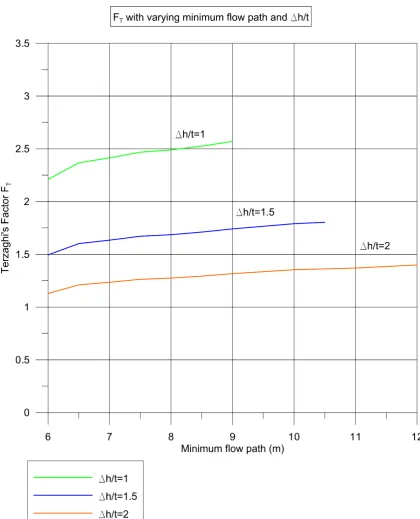
To better illustrate this effect, the analyses were repeated for variations in the

minimum flow paths, achieved by increasing gradually the height of the soil retained

behind the retaining wall. The calculated values of Terzaghi’s factor are plotted in

Figure 6 against the minimum flow path for the different ratios of h/t. It can be seen

that the minimum flow path is 6m for the cofferdam case, regardless of the level of the

water behind the wall, while for the 10m deep excavation, the minimum flow path was

Moreover, for the same h/t, the Terzaghi’s factor becomes lower as the minimum flow

path decreases with the cofferdam case being the most critical.

Effect of excavation width

In this section, the effect of varying the excavation width on the calculated Terzaghi’s

factor is investigated for the two reference geometries in Figure 2.

Figure 7 shows head equipotential lines for three cases: (a) a wide excavation

(width x=12t), (b) a narrow trench (x=t), and (c) a circular excavation (diameter d=t). In

all cases, the seepage is generated from a side boundary located at 18m (6t) from the

wall, where a constant head is applied. For h=1.5t, the Terzaghi’s factor of safety FT

is: (a) 2.89; (b) 1.33 and (c) 0.97, respectively (Simpson and Katsigiannis 2015).

Similarly, Aulbach and Ziegler (2013) found that when water is flowing

upwards, beneath a narrow excavation, the upward hydraulic gradients are higher than

in the cases of wider excavations with little or no lateral restraint.

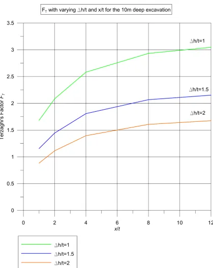
To better illustrate this effect, the analysis is repeated for different x/t ratios

where x is the excavation width in the horizontal direction (only half the excavation is

modelled due to symmetry) and t is the embedment depth in the vertical direction while

the rest of the model parameters remain the same. More specifically, 5 different cases

were considered for plain strain conditions: x/t=12, 8, 4, 2 and 1. At the end of each

analysis, the Terzaghi’s factor was calculated using the values of the pore water

pressures acting at the bottom of the soil block from the output of the calculations. This

study includes 10 different geometries each simulated using three different values of

h/t, totalling 30 analyses.

In Figure 8, the Terzaghi’s factor is plotted against the ratio x/t for h/t=1.5. It

can be seen that, the narrower the excavation is, the lower the factor of safety becomes.

geometries. Figure 9 presents the values of the Terzaghi’s factor for different values of

x/t and h/t for the excavation case. Again, it can be seen that the factor of safety drops

significantly as the excavation becomes narrower.

Discussion

It can be concluded that the use of the Soil Block approach with FE methods is

straightforward, requiring only the pore water pressure from the numerical analysis for

the calculation of the Terzaghi’s factor of safety. The calculated Terzaghi’s factor

directly depends on the upstream and downstream groundwater levels as specified by

the ratio h/t. It was also noted that for a given difference in the hydraulic head, the

system becomes more critical for shorter minimum flow paths and narrow excavations,

where confined spaces result in an increase in the groundwater pressures.

The obvious disadvantage of the Soil Block Approach is that it provides no

useful information about the critical failure mechanism and it is only applicable to very

specific situations of upward flow towards a horizontal surface. In practice, more

complex situations are encountered, including flow beneath sloping surfaces in

embankments and cuttings.

The Integration Point Approach

The second approach for verifying stability against HYD using FEM, is the integration

point approach which can be expressed in two different forms, depending on how

safety is introduced into the calculations. According to EC7, design ground-water

pressures may be derived either by applying partial factors to characteristic water

pressures or by applying a safety margin to the characteristic water level (BS EN1997-1

In the first form of the Integration Point Approach, safety is verified at every

integration point for a given set of partial load factors applied to the destabilising and

stabilising actions. Hence, the design water pressures are calculated after applying the

corresponding factor to their characteristic values, derived from the output of the FE

calculations.

In the second form, no factors are applied to the water pressures but their design

values are derived by directly assessing the design water table which is input in the

numerical calculations. Thus, the values derived from the output of the FE analysis are

already design values and no further factors need to be applied. Afterwards, the

stabilising and destabilising pressures are combined at every integration point to give

the achieved factor of safety as an estimate of the level of safety and economy.

In both cases, as outputs of the numerical analysis are used for the safety

verification, care must be taken when selecting the appropriate boundary conditions and

mesh coarseness as these will affect the calculated values.

Apply partial factors to the excess pore water pressures

In the first form of the approach, stability is verified at every integration point by

checking that a relevant criterion with a given combination of partial factors, is fulfilled

for a soil column of negligible width above each point. Then contours of the criterion

values can be plotted downstream, in front of the wall, to check whether the criterion is

fulfilled.

Simpson (2012) shows that when water pressures have to be factored, dst should

be applied to the excess pore water pressure because the destabilizing seepage force is

only caused due to the excess pore water and not the hydrostatic component of the water

pressure. Similarly, the stabilising factor, stb should be applied to the buoyant density of

criteria, namely the and , defined in Equations 6 and 7 respectively. The values of

the partial factors and , used in both Equations, correspond to the values

required by EC7 and are given in Table 2.

(6)

(7)

The difference between the two criteria is that in , the total vertical stress, v

is equal to , while in the v value is taken from the output of the numerical

analysis (i.e. it includes other elements such as friction). No evidence is presented in the

literature on which criterion is more suitable. Stelzer and Odenwald (2015) used the

criterion (referred to as simply D in their paper) for verifying safety against HYD for a

cofferdam geometry as a way to take into consideration the stress redistribution and the

friction. However, a thorough comparison of the two criteria is needed to better

understand their advantages and limitations.

In Figures 10 to 13, the contours of the and criteriaare presented for the

two extreme cases considered in section 4: the 10m deep excavation and the cofferdam

case with x/t=4. For illustration purposes, only the contours for the cases that

correspond to a Terzaghi’s factor equal to 1.5 are presented here. It can be seen in

Figure 6, that the Terzaghi’s factor becomes 1.5 for h/t=1.8 and h/t=1.5 for the 10m

excavation and the cofferdam case respectively. This is because the minimum flow path

is shorter for the cofferdam geometry and hence the hydraulic heave problem becomes

Note that the contours are only plotted for the area of interest in front of the

wall, where the vertical dimension of the area in the y axis direction, is twice the

embedment depth and the horizontal dimension in the x axis direction is half the

excavation width.

It can be seen from Figure 10 and Figure 11 that while both cases correspond to

a value of Terzaghi’s factor equal to 1.5, when the contours of are plottedusing the

partial factors required by EC7 (where dst/ stb=1.5), there is an area close to the wall

where the safety criterion is not fulfilled (zone with negative values).

In Figures 12 and 13, the contours of are plotted using again the EC7 partial

factors and the effect of using the v values from the output of the FE analysis instead of

z, is illustrated. For the 10m excavation case, it can be seen from Figure 12 that the

contours of are everywhere positive and the criterion everywhere fulfilled. This

means that using v instead of z to calculate the stabilizing stresses has a significantly

favourable effect. On the other hand, for the cofferdam case, when the contours of

are plotted (Figure 13), it is observed that while the negative area is smaller compared

to the contours of in Figure 11, the criterion is still not fulfilled everywhere. It is

obvious that while z is uniquely defined, v variesand can have a favourable effect

when being used instead of z.

Please note that negative values of either D or D relate to a local failure at the

specific integration point and not to the global failure of the soil in the area in front of

the wall. That is why an essential part of the HYD verification using the Integration

Point approach is the contour plotting of the criteria values.

Direct assessment of the design water table

pressures (Evolution Group 9 - Water Pressures, 2014). The members of EG9 have

recommended that in situations of this type, partial safety factors should not be applied

to water pressures or to forces derived from water pressures, such as the seepage force

S. Instead, engineers must take an appropriately cautious view of the piezometric water

table level and the water pressures that could occur in the ground. According to EG9,

the characteristic piezometric water levels and accordingly the characteristic values of

water pressures shall correspond to a return period at least equal to the duration of the

design life span of the structure (e.g. 100 years) while the ultimate limit state

piezometric water levels and accordingly the ultimate limit state values of water

pressures shall have a rare probability (e.g. 1%) of occurrence in the duration of the

design situation of the structure. This also implies that a careful review of the possible

range of distributions of permeability must be undertaken (e.g. even thin layers of lower

permeability can cause the generation of high water pressures)and the design must be

based on the worst that is credible.Afterwards, the code requirement is simply to prove

that equilibrium exists under those design conditions.

An alternative form of the integration point approach, described previously, can

be used in combination with such directly specified design water table, to give an

estimate of the achieved level of safety at every integration point of the FE mesh in the

area in front of the wall. Based on the definitions of and (Equations 6 and 7), the

integration point approach factors of safety, namely and are defined in

Equations 8 and 9.

(8)

According to these definitions, and are equal to the ratio dst/ stb when

the criteria D and D respectively, are equal to zero. Hence, the contours of and

, provide the safety factor value achieved at each integration point. Again, the two

Equations differ in the way they include the total vertical stress in the calculations.

Equation 8 ignores the mobilised friction effects whilst Equation 9 introduces v directly

from the output of the FE analysis, hence accounting for the friction developed along

the soil/wall interface.

In Figures 14 and 15, the contours of are plotted for the 10m deep

excavation and the cofferdam case for a ratio of h/t equal to 1.8 and 1.5 respectively. It

can be seen that, in both cases, a minimum value of equal approximately to 1.3 is

achieved. The lowest value of the factor of safety is close to the toe of the wall where

the excess pore water pressures have their highest values.

Similarly, in Figures 16 and 17, the contours of are plotted for the same

cases. However, the calculated values of the safety factor are now different for the two

problems. For the 10m excavation case, the minimum factor is 1.8 (see Figure 16) while

for the cofferdam case it is 1.4 (see Figure 17). Both values are higher than the

corresponding minimum value observed in Figure 14 and 15 for the same h/t.

However, is much higher for the 10m excavation than the cofferdam case because

of the favourable effect of the mobilised friction.

Comparison of the factors

It was observed above that for cases corresponding to a Terzaghi’s factor of 1.5,

there is an area close to the wall where is less than 1.5, while when calculating the

values, it was observed that the factor varies depending on the effect of the

between the calculated values of the safety factors from the Soil Block and the

Integration Point approaches, together with a better understanding of the resulting

differences.

In this section, the minimum integration point factors and (i.e. close to

the toe of the wall) are plotted against the Terzaghi’s factor FT for the 10m excavation

and cofferdam cases with varying x/t, h/t and the soil/wall interface friction angle . In

Figure 18, the relationship between and FT is presented. As can be seen, the points

follow a linear trend, where FT = 1.15 , with an R2 value of 0.98. Since friction is not

considered, only one line defines the relationship between the two factors. According to

their definition, both factors are calculated using z as the stabilizing stress. However, as

the factor is calculated at every integration point of the FE mesh, instead of a soil

block, a value of 1.0 is only related to a very local failure at the specific integration

point and not the global failure of the soil in the area in front of the wall.

In Figure 19, the relationships are given between the Terzaghi’s factor FT and

the integration point approach factor, for both geometries. Straight lines are a good

approximation (with R2 values between 0.89 and 0.98). However, due to the presence of

friction, the relation is not unique. is higher for the 10m excavation case than the

cofferdam case as the friction effect is more significant. When tan increases from

0.5tan ’ to tan ’, both lines move to the right as values increase (dashed lines).

The reason for this is that the effective horizontal stresses acting on the wall, and

therefore, the mobilised friction, are different. While the earth coefficient at rest is the

same and equal to 1-sin ’, the initial effective horizontal stresses are different as they

are calculated at different depths. Since the initial stresses are calculated before the

excavation is made, the toe of the wall is 13m and 3m below the ground level for the

of soil, the horizontal effective stresses are ‘locked-in’. They don’t completely

disappear when the loading is removed.

To illustrate this effect, Figure 20 presents the effective horizontal stress profiles

in front of the wall and the resultant forces for all cases. It can be noted, that the

effective horizontal stresses are much higher for the 10m excavation than the cofferdam

case. Moreover, when tan increases from 0.5tan ’ to tan ’, the total force increases

from 13.1kN/m to 21.8kN/m in the case of the cofferdam and from 69.4kN/m to

137.5kN/m in the case of the 10m deep excavation. This increase in horizontal stresses

is directly proportional to the friction between soil and wall. The findings agree with the

results of Benmebarek et al. (2005) who carried out parametric analysis to investigate

the effect of wall friction for a similar problem and Stelzer and Odenwald (2015) who

observed a higher effect of friction in a supported excavation, when compared to a

cofferdam geometry, resulting in higher stresses in the proximity of the wall.

The analysis was also repeated for a weaker soil to investigate the effect of the

soil strength parameters on the calculated values of and and the relationship

with FT. The new soil has an angle of shearing resistance equal to ’=25 while the rest

of the soil parameters, listed in Table 2, remain the same. The analysis is repeated for

both the 10m excavation and the cofferdam case with varying h/t, x/t and .

Since is not related to the friction angle but to the unit weight of the soil,

the relationship determined in Figure 18 can be used for this soil. However, as

illustrated in Figure 21, the effect is significant for . It can be seen that the solid

lines for the 10m excavation and the cofferdam case, have moved to the left of the

graph and hence the values have decreased when compared to Figure 19. The

decrease in the angle of shearing resistance and hence the decrease in soil/wall friction

effect on the calculated values. It is worth noting that when tan increases from

0.5tan ’ to tan ’, both lines move to the right as values increase (dashed lines).

The effect is again particularly significant for the 10m excavation case where v is much

higher than z due to the friction component. It is important to mention that all the other

geometries considered, for the minimum flow path parametric analysis, yielded values

that fell between the lines in Figures 19 and 21.

In all cases considered, for the same FT value, the calculated values of are

higher than the corresponding values of , meaning, in principle, that v> z. As the

effect of friction becomes more significant, either by increased effective horizontal

stresses or soil/wall interface friction angle , v becomes much higher than z and

hence is muchhigher than .

However, it is interesting that the range of values, from all cases considered,

narrows down for lower values of FT (especially lower than 1.5) and also their values

become closer to the corresponding values. In fact, they almost have a common

point at = =1, FT =1.15.At this point, friction against the wall is destroyed by

water pressure.

Discussion

The results show that there is a unique and simple relationship between FT and FD,

proportional to the unit weight of the soil. With regards to the calculations using

two extreme geometries, two different angles of shearing resistance ’ and soil/wall

interface friction angles , have shown that the range of relationships between the

factors is broad and very sensitive to effect of friction along the wall.

Moreover, the values are lower than those of for all cases considered

when pore water pressures rise, the effective stresses decrease and the friction effect is

lost. In this instance, the HYD Limit State becomes more critical and all the lines

tend to converge towards the line.

The use of the factor of safety presents advantages over the use of the

factoras, in general, designers should not just rely on the favourable friction effect to

verify stability against HYD. Remote from the limit state, wall friction appears to

enhance safety, increasing . But at the limit state, this is no longer so because the

water pressure destroys the friction. This illustrates the fact that carrying out

calculations for conditions remote from the limit state and then relying on a factor of

safety can be misleading.

Concluding remarks

The verification of stability against HYD using FE methods is straightforward and

seems very promising. While designers might be more familiar with the Soil Block

approach and the Terzaghi’s calculation, the more advanced Integration Point approach

has the advantage that it is readily applicable not only to the simple cases considered

here, but also to more complicated situations such as water approaching sloping ground

surfaces. Moreover, it provides insights about the stability of the soil at a very local

level, instead of assuming a pre-defined failure mechanism (e.g. a block of soil mass

with specific dimensions).

There are two ways to introduce design values of the destabilising pore water

pressures into the Integration Point approach calculations; either by applying the HYD

partial load factors suggested by EC7 to the characteristic values or by directly

assessing the design water table. As it is very likely, based on the suggestions of the

7, due in 2020, will move away from factoring the pore water pressures, the calculation

of the integration point factors, based on a direct assessment of the groundwater

conditions, might become more relevant in the future compared to the verification using

the and criteria, which involve the application of partial factors. Moreover, the

integration point approach criteria and factors of safety are calculated based on the

excess pore water pressures. Therefore, the Integration Point approach addresses the

misinterpretation mentioned above regarding which component of the pore water

pressure needs to be factored.

The use of the safety factor to get an estimate of the safety margin has

significant advantages, in the opinion of the authors, since there is no friction available

at the limit state.

Further research

This paper presents a comprehensive study on the subject focusing on plain strain

two dimensional problems. Further studies need to address the applicability of the

conclusions for axi-symmetry problems (e.g. circular excavations). Moreover, Aulbach

and Ziegler (2014) have investigated that hydraulic heave is most critical in the corners

of excavation pits. Therefore, a further study should also examine whether the

conclusions are also applicable for 3D problems.

Acknowledgements

The authors gratefully acknowledge the support of the project partners, EPSRC and

Arup. Special thanks are extended to Brian Simpson from Arup Geotechnics and the other

References

Aulbach, B., and Ziegler, M. 2013. Simplified design of excavation support and shafts

for safety against hydraulic heave. Geotechnics and Tunnelling, 362-374.

Aulbach, B., Ziegler, M. 2014. Versagensform und Nachweisform beim hydraulischen

Grundbruch – Plädoyer für den Terzaghi-Körper, Geotechnik, 6-18.

BAW. 2013. Code of Practice: Internal Erosion (MMB). German Federal Waterways

Engineering and Research Institute, Karlsruhe

Benmebarek, N., Benmebarek, S., and Kastner, R. 2005. Numerical studies of seepage

failure of sand within a cofferdam. Computers and Geotechnics, 264-273.

BS EN1997-1, Eurocode 7 – Geotechnical design, Part 1 – general rules. 2004. London:

British Standards Institution.

Das, B. 1983. Advanced Soil Mechanics. McGraw-Hill.

Davidenkoff, R.N. 1954. Zur berechnung des hydraulischen grundbruches.

Wasserwirtschaft 1954(46):298–307.

Evolution Group 9 - Water Pressures. 2014. Final report to TC250/SC7 Evolution of

Eurocode 7 Part 1. July 2014.

Harr, M. 1962. Groundwater and Seepage. McGraw-Hill.

Kashef, A. 1986. Groundwater Engineering. McGraw Hill.

Marsland, A. 1953. Model experiments to study the influence of seepage on the stability

of a sheeted excavation in sand. Géotechnique. The Institution of Civil Engineers.

London 1953; 4(7):223–41.

McNamee, J. 1949. Seepage into a sheeted excavation. Géotechnique. The Institution of

Civil Engineers. London 1949; 4(1):229–41.

Odenwald, B., and Stelzer, O. 2013. Nachweis gegen hydraulischen Grundbruch mit

FEM auf Grundlage des EC 7. Workshop Bemessen mit numerischen Methoden (pp.

88-110). Veröffentlichungen des Institutes Geotechnik und Baubetrieb TU Hamburg

Orr, T. 2005. Model Solutions for Eurocode 7 Workshop Examples. Dublin: Trinity

College.

Ryner, A., Fredriksson, A., and Stille, H. 1996. Sponthandboken: handbok f̈r

konstruktion och utformning av sponter. Byggforskningsr̊det T18:1996.

Simpson, B., Blower, T., Craig, R.N. and Wilkinson, W. B. 1989. The engineering

implications of rising groundwater levels in the deep aquifer beneath London. CIRIA

Simpson, B., Morrison, P., Yasuda, S., Townsend, B., and Gazetas, G. 2009. State of the

art report: Analysis and design. Proc. 17th Int. Conf. SMGE, Alexandria, Vol 4, pp.

2873-2929.

Simpson, B., Vogt, N. and Van Seters, A.J. 2011. Geotechnical Safety in Relation to

Water Pressures. Proceedings of the 3rd International Symposium on Geotechnical

Safety and Risk. Munich.

Simpson, B. 2011. Water pressures. Proc. 2nd International Workshop on Evaluation of

Eurocode 7. Pavia. 12-14 April 2010.

Simpson, B. 2012. Eurocode 7 – fundamental issues and some implications for users.

16th Nordic Geotechnical Meeting (pp. 29-52). Copenhagen: Danish Geotechnical

Society.

Simpson, B., and Katsigiannis, G. 2015. Safety Considerations for the HYD Limit State.

XVI European Conference on Soil Mechanics and Geotechnical Engineering (pp.

4325-4330). Edinburgh: ICE Publishing.

Skempton, A. W., and Brogan, J. M. 1994. Experiments on piping in sandy gravels.

Géotechnique. 44, No. 3,449-460.

Stelzer, O., and Odenwald, B. 2015. A New Stress-Based Approach for Verification of

Safety Against Hydraulic Heave Based on EC7. XVI European Conference on Soil

Mechanics and Geotechnical Engineering (pp. 4073-4078). Edinburgh: ICE Publishing.

Stroud, M.A. 1987. The Control of Groundwater. General Report and State of the Art

Review to Session 2 of IX ECSMFE Dublin.

Terzaghi, K. 1922. Der Grundbruch an Stauwerken and seine Verhiltung. Die

Wasserkraft, 445-449.

Terzaghi, K. 1943. Theoretical Soil Mechanics. New York: J. Wiley and Sons.

Terzaghi, K., Peck, R., and Mesri, G. 1996. Soil Mechanics in Engineering Practice, 3rd

edition. John Wiley & Sons, Inc.

Williams, B., and Waite, D. 1993. The design and construction of sheet-piled cofferdams.

London: Special publication 95. Construction Industry Research and Information

Table 1. Partial factors for HYD

Action Symbol Value

Permanent

Unfavourablea

Favourableb

G;dst

G;stb

1.35

0.90

Variable

Unfavourablea Q;dst 1.50

a Destabilising b Stabilising

Table 2. Mohr-Coulomb model parameters

Soil Properties

Young’s Modulus, E' ( Pa) 25+6.5z

Angle of shearing resistance, ' (°) 35

Effective cohesion, c' (kPa) 0

Poisson’s ratio, ' 0.2

Permeability (m/s) 10-5

Table 3. Published values for Terzaghi’s factor of safety FT (update of the table given by

Simpson & Katsigiannis, 2015)

Publication and any limitations Values

Williams & Waite (1993)

For clean sands

1.5 to 2.0

Kashef, Abdel-Aziz Ismail (1986) 4 to 5

Harr (1962) 4 to 5

German practice – unfavourable soils

(DIN 1054/A2 2015-11) – favourable soils

2

1.53

Swedish practice – coarse soils

(Ryner et al 1996) – silty material

1.5

2.5

Dutch practice 2.8

Figure 1. Example of situation where heave might be critical

Figure 3. Finite Element mesh for the 10m deep excavation model

Figure 18. Relationship between the Terzaghi’s factor FT and the integration point

Figure 19. Relationship between the Terzaghi’s factor FT and the integration point

Figure 21. Relationship between the Terzaghi’s factor FT and the integration point