City, University of London Institutional Repository
Citation:
Kovacevic, A., Stosic, N. and Kethidi, M. (2014). Deforming grid generation and CFD analysis of variable geometry screw compressors. Computers & Fluids, 99, pp. 124-141. doi: 10.1016/j.compfluid.2014.04.024This is the accepted version of the paper.
This version of the publication may differ from the final published
version.
Permanent repository link:
http://openaccess.city.ac.uk/12665/Link to published version:
http://dx.doi.org/10.1016/j.compfluid.2014.04.024Copyright and reuse: City Research Online aims to make research
outputs of City, University of London available to a wider audience.
Copyright and Moral Rights remain with the author(s) and/or copyright
holders. URLs from City Research Online may be freely distributed and
linked to.
1
Deforming Grid Generation and CFD analysis of Variable
Geometry Screw Compressors
Sham Rane*, Ahmed Kovacevic, Nikola Stosic, Madhulika Kethidi
Centre for Positive Displacement Compressor Technology,
City University London, EC1V 0HB, London, U.K. email: [email protected]* Corresponding Author Tel: +44(0) 20 70408395, Fax: +44(0) 20 70408566
Abstract
The most common type of twin screw machines are twin screw compressors. These normally contain
rotors of uniform pitch and profile along the rotor length. However, in some cases such as in twin screw
vacuum pumps with very large pressure ratios, the variable pitch rotors are often used to improve
efficiency. The limited use of rotors with variable pitch and/or section profile is mainly due to
manufacturing constraints. In order to analyse the performance of such machines by means of
Computational Fluid Dynamics (CFD), it is necessary to produce a numerical mesh capable of calculating
3D transient fluid flows within their working domains.
An algebraic grid generation algorithm applicable to unstructured grid, Finite Volume Method (FVM) for
variable pitch and variable profile screw machines is described in this paper. The grid generation
technique has been evaluated for an oil free air compressor with “N” profile rotors of 3/5 lobe
configuration. The performance was obtained by calculations with commercial CFD code. The grid
generation procedure provides mesh of the required quality and results from CFD calculations are
presented to compare performance of constant pitch rotors, variable pitch rotors and variable profile
rotors. The variable pitch and variable profile rotors achieve steeper internal pressure rise and a larger
discharge area for the same pressure ratio. Variable Pitch rotors achieve reduced sealing line length in
high pressure domains.
Keywords: Algebraic Grid Generation, Computational Fluid Dynamics, Twin Screw Compressor,
2 Nomenclature:
L – Rotor Length
D – Male Rotor Outer Diameter
Φw – Male Rotor Wrap Angle
α – Male rotor rotation angle
Δα – Increment in Male rotor rotation angle
Z – Axial distance along the rotors
ΔZ – Increment in Axial distance
z1 – Number of lobes on the Male rotor
z2 – Number of lobes on the Female rotor
i – Rotor Gear ratio = z2/z1
ps – Starting Lead
pe – Ending Lead
ja – Grid density in axial direction per interlobe
x – X coordinate
y – Y coordinate
r – Radius
θ – Angle turned by male rotor
r.p.m – Male rotor speed
t – Time
Δt – Time Step Size
Vi – Built in Volume Index
Abbreviations:
CFD – Computational Fluid Dynamics
FVM – Finite Volume Method
SCORG – Screw Compressor Rotor Grid
Generator
PDE – Partial Differential Equation
TFI – Transfinite Interpolation
GGI – Generalized Grid Interface
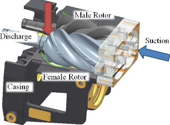
1 Introduction
Screw compressor rotors are effectively helical lobed gears with profiles developed for
optimized compression process. The compressor working chamber is formed by the space
contained between the intermeshing rotors and the casing which decreases is size as they rotate.
3 compression process, leakage flows, heat transfer, oil injection and other phenomena of interest
for compressor design occur within that space. To achieve efficient compression the clearances
between the rotors and between the rotors and the casing must be minimised. For oil injected
compressors these can be as small as 40 μm but for dry compressors these may have to be of the
order of hundreds of micro meters to allow for thermal expansion. Regardless of the type of
compressor and depending on the size of the machine, the working chamber main dimensions
can be of the order of 1000 times larger than these values. This complicates the task of creating
numerical meshes capable of such a dimensional variation. This is further exacerbated by the
transient nature of the process, high pressure and temperature gradients, and domains with a
variety of flow regimes.
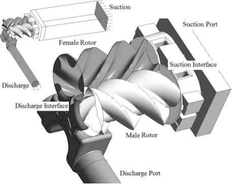
Fig. 1. Oil free Twin Screw compressor and its working chamber
Grid generation for numerical simulation of 3D flow processes requires the domain to be broken
up into a number of regularly shaped discrete volumes with computational points in the centre of
each. In order to obtain boundary conformal representation of physical space, most grid
generation techniques start from the boundaries and proceed to the interior. There are three main
classes of mathematical techniques used for this process, a) Algebraic methods, b) Differential
Methods and c) Variational methods. Authors such as [20, 29, 30] have described different grid generation techniques in detail. Shih et al [24] reviewed different types of grids and their relative advantages.
Algebraic methods are direct and depend on the use of parametric functions to discretize the
boundaries and then use interpolation to calculate interior points. They are suitable for regular
geometries and structured grids and have relatively simple implementation. Numerical grids are
4
25, 26 ] have described various aspects of algebraic grid generation such as the control point form, transfinite interpolation techniques, grid adaptation, weighting functions for multivariable
adaptation etc.
Differential methods are indirect and more suitable for complex geometries. They depend on the
solution of partial differential equations. These can be elliptic, parabolic or hyperbolic in nature
and their selection depends on the geometry to be discretized. Boundary discontinuities can be
avoided to extend to the interior points, but they require significant computational effort and time
to solve.
Variational methods depend on such measures of the grid quality as orthogonality and skewness.
Using them, the computational points can be distributed to optimize a function of the grid
quality. However, they have complex formulations and are difficult to control.
Methods for grid generation in screw compressor applications need to be easy to implement and
quick. Analysis of the working chamber is transient in nature and requires a grid to represent a
rotor position for every time step, taking into account the change in size of the working domain.
In this respect, algebraic methods can recalculate the grid quickly. In [10, 11], Kovacevic et. al.
have successfully used an algebraic grid generation method together with boundary adaptation
and transfinite interpolation. This has been implemented in the custom made program for the
calculation of a screw compressor numerical mesh called SCORG. Kovacevic in [16] presented the grid generation aspects for twin screw compressors in detail. In [12, 13, 14, 15, 17 and 18],
Kovacevic et. al. have reported CFD simulations of twin screw machines for the prediction of flow, heat transfer, fluid-structure interaction, etc.
The use of a differential method requires the solution of a PDE for every rotor position. The grid
5 solution. Also there is little control available for the solution of these PDE’s. Voorde et. al. in [31, 32] developed an algorithm for conversion of an unstructured grid to a block–structured mesh for twin screw compressors and pumps from the solution of the Laplace equation. Apart
from these works, there are only a few reports available on transient three dimensional CFD
analyses of screw machines. All these developments were concentrated on machines with
uniform pitch rotors and so far no published work is available on the numerical analysis of twin
screw compressors with variable pitch or variable profile rotors.
The use of general purpose grid generators for screw compressors has been found to be
inadequate [18, 21, 22] and only customized grid generation programs are available for twin screw compressor applications. The motivation for the present work was to develop existing
functionality to handle grid generation of twin screw rotors with variable pitch and variable
section profiles so that CFD simulations of these new types of machines is possible.
Numerical treatment of the CFD models for screw compressors with uniform lead and variable
lead rotors differs mainly at the grid generation stage. In the grid generation technique for
constant pitch rotors the axial distance between the grid points is constant. The challenge in
generating a grid for variable lead rotors is that the axial distance and angular rotation of nodes
change continuously. To accommodate this change, the grid needs variable spacing in the axial
direction which will still provide a conformal mesh. This topology remains the same over the
entire length of the rotor but the rotors change their relative position governed by the variable
lead. Apart from that, the grid generator has to accommodate the large difference in length scales
6 2 Uniform versus Variable Pitch
Although there is a patent by Gardner [7] on continuously variable pitch rotor dated back to 1969, such machines are not used much and are still in the research phase. The patent proposes a
helical screw compressor with continuously variable lead for both rotors, male and female. Due
to the lack of manufacturing techniques to produce such rotors, Gardner proposed forming them
from a stack of metal plates with different leads which is still used today in some designs of
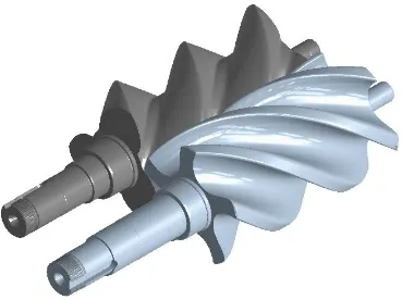
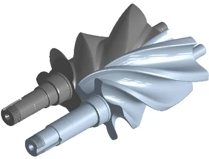
vacuum pumps. Fig. 2 shows twin screw rotors with uniform pitch whereas Fig. 3 shows twin
screw rotors of the same size but with variable pitch. It has been shown in literature that for the
same rotor lengths, diameter, wrap angles and lobe profiles, variable pitch rotors can be designed
to provide higher pressure ratios and larger discharge port opening areas with reduced throttling
losses when compared to constant pitch rotors [7].
Fig. 2. Meshing of Uniform Pitch Twin Screw
Rotors
Fig. 3. Meshing of Variable Pitch Twin Screw
Rotors
As confirmed by many authors, screw compressor efficiency depends upon the profile of the
rotors, the combination of male and female lobes, the length and diameter, the wrap angle and
the rotor clearances [5, 6, 8]. Based on these and the original work of Gardner [7] it is suggested that the effects of variable lead rotor designs are as follows;
a) If all other variables are unchanged for a constant lead rotor pair and a variable lead rotor
pair, the length of the sealing line will be less for the variable rotor pair as the rotor lead
reduces from suction to discharge. Since the leakage loss is directly proportional to the
7 high pressure regions, the leakage loss will be reduced. This may lead to higher
volumetric efficiencies with variable lead rotors.
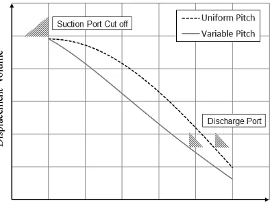
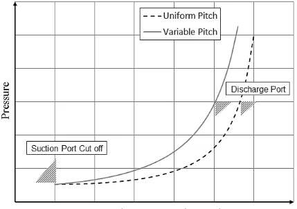
b) For variable lead rotors, the reduction of volume during the compression process will be
faster than for constant lead rotors, as shown in Fig. 4. Consequently the pressure will
rise more rapidly for the variable lead rotors as shown in Fig. 5.
c) The built-in volume index is the ratio of the suction closure to the discharge opening
volumes. The suction volume is the maximum volume at which the suction port is usually
closed and where the compression process begins. The discharge volume is the size of the
compression chamber at the moment of opening of the discharge port. As shown in Fig.
4, to achieve the same Vi for variable pitch rotors the discharge port should be opened
earlier which allows it to be bigger than in the constant lead case. Hence it is possible to
have a greater discharge area at a similar pressure ratio and this will reduce the throttling
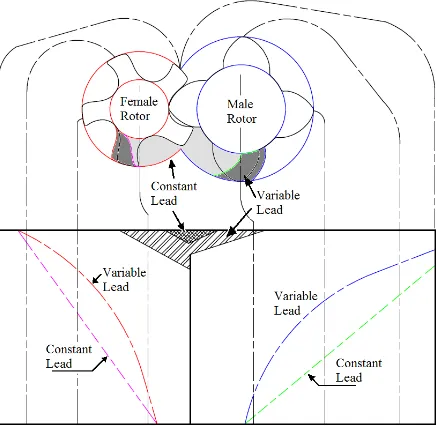
losses. Fig. 6 shows the radial and axial ports for the variable and constant lead rotors in
order to demonstrate the difference in size of the ports with the same Vi and discharge
pressure.
Fig. 4. Volume-Angle diagram Fig. 5. Pressure-Angle Diagram
d) If the same size of discharge port is retained for both the variable and uniform lead rotors,
the discharge pressure of the variable rotors will be higher. This indicates that variable
lead rotors can achieve a higher Vi index.
8 However, a variable lead compressor with the suction port in the same position as in a uniform
lead compressor may have a reduced capacity.
The advantages and disadvantages identified on the basis of previous research have not been
tested so far on physical prototypes due to difficulties in producing such rotors with existing
manufacturing methods. However, these can be investigated further in detail by use of CFD
analysis if an appropriate numerical mesh can be generated. The arguments b, c and d presented
above are applicable even for variable profile rotors designed such that the flow area is reduced
continuously from the suction to the discharge end of the rotors.
3 Grid Generation for uniform pitch screw rotors
The screw compressor working domain is spatially discretized by use of both, structured and
unstructured grids. The flow domains of the screw compressor consist of the rotor domain, the
suction port and the discharge port.
Fig. 7. Twin screw compressor working chamber domains
Fig. 7 shows a complete grid of the compressor model. The suction and discharge ports can be
meshed by use of general purpose grid generators in which case it is easier to generate a
tetrahedral unstructured grid with fine prism layers covering the boundaries. The customized grid
generator [18] is used for the generation of a structured hexahedral mesh consisting of two sub-domains each belonging to one of the rotors. The rotor mesh changes for every time step, causing
deformation of the generated finite volumes and sliding on the interfaces. The sole reason for the
use of the customized grid generator for a screw compressor is that unstructured meshes do not
9 compressors [22]. These tetrahedral meshes of the ports and the hexahedral meshes of two rotor subdomains are connected by non-conformal GGI interfaces in the solver.
Fig. 8. Simplified Block Diagram of Screw Compressor Rotor Grid Generator
Hexahedral meshes for the rotor domains are generated by the use of an algebraic grid generation
method employing multi parameter one dimensional adaptation and transfinite interpolation. Fig.
8 shows a simplified block diagram of the steps performed in the screw compressor rotor grid
generator. The topology of the flow domain between the male rotor, female rotor and the casing
resembles a ∞ figure. In order to simplify the grid generation process, the entire rotor domain is
subdivided in two regions each belonging to one of the rotors. These domains are separated by
the rack, a curve which uniquely separates both domains [27]. By this means an “O” grid is constructed for each rotor domain.
Consecutive 2D cross sections are calculated individually using the following steps [16]:
• Transformation from the ‘physical’ domain to the numerical domain.
• Definition of the edges by applying an adaptive technique.
• Selection and matching of four non-contacting boundaries.
• Calculation of the curves, which connect the facing boundaries by transfinite
interpolation.
• Application of a stretching function to obtain the distribution of the grid points.
• Orthogonalisation, smoothing and final checking of the grid consistency.
This procedure is the most important function of the framework and provides flexibility to
10 The rack generation procedure, using a primary curve to specify both rotor profiles, is described
in detail by Stosic in [27, 28].
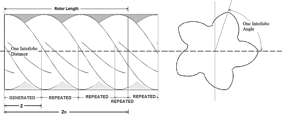
With reference to Fig. 9, the interlobe angle is the angle which the male rotor needs to rotate to
get one lobe in the position of the next one. This angle is equal to 2π / z1. The interlobe angle of
the female rotor is proportional to the male interlobe angle by the ratio of z1 / z2. After each
interlobe angle rotation, the rotors come into geometrically identical position to the starting
position. Hence the grid vertex positions can be reset to the starting position after each interlobe
angle rotation and renumbered, as required, to maintain progressive rotation. Similarly the same
set of generated cross sectional meshes can be repeated along the rotor axis with appropriate
renumbering of the nodes and cells. Angular rotation of the rotor covering one interlobe angle is
discretized into jadivisions and each angular increment is then equal to Δα = (2π / (ja z1)). This
angular increment is the governing factor for the size of the time interval in a transient
simulation. The 2D grids for each of cross sections are generated using the above principle and
the functionality shown in flow chart Fig. 8 and are stored in the vertex coordinate files.
Fig. 9. Uniform Pitch Grid Generation
Due to the constant helix angle the axial distance between cross sections corresponds to the
angular rotation of the rotor. As shown in Fig. 9, one interlobe angle corresponds to the axial
rotor length of one pitch. Due to this correlation the structure of 3D data will consists of
repeating blocks of data with updated indexing of the vertices which are generated only once for
the first interlobe. During this stage, the hexahedral cell connectivity will also be established for
the first generated section by use of 4 nodes from one cross section and the remaining 4 nodes
from the neighbouring section. All other axial grid sections will be repeated and equally spaced
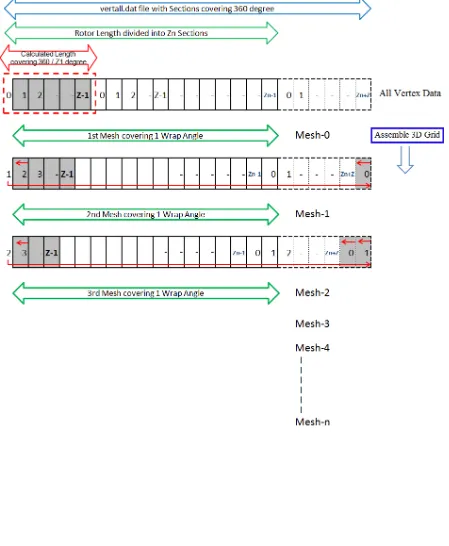
11 Transient simulation of the fluid flow requires that the external mesh, representing the domain
for all time steps is available and the appropriate mesh is imported in the solver at the beginning
of each time step. This process is shown in the block diagram in Fig. 10. The mesh representing
the initial position is written with all data for Zn numbers of sections. For the next time step, the
grid is re-indexed so that the cross sections are moved for one ΔZ interval and the front cross
section is stacked at the end position. In other words, this is achieved by re-indexing the nodes
for all the cross sections so that indices of the previous section are associated with the next one
taking all into account, from the first to the last section.
Since all cross sections are at the constant distance ΔZ the fixed angular increment Δα will
represent constant rotational speed. The time step size for the entire simulation is constant and
defined as Δt = 60.0/ (rpm ja z1).
Fig. 10. Uniform Pitch Rotor Grid Assembly in 3D
4 Grid Generation for variable pitch and variable profile screw rotors
For the Uniform Pitch rotors, there is a fixed relation for the axial distance between the cross
sections and the unit rotation angle over the entire length of the rotor. This is convenient because
the profile is constant and the grid generated for one interlobe space can be reused in consecutive
interlobes. However, for rotors of variable pitch, this relation varies along the length of the rotor.
Therefore it is impossible to use the same method with a constant axial distance between sections
for grid generation of such rotors. At the same time the rotors need to rotate at a constant angular
speed similar to the rotors of constant pitch. In such a case the angular and axial intervals for grid
definition do not relate directly to the angular rotation. Fig. 11 shows the grid difference between
12
Fig. 11. Axial spacing difference between uniform pitch and variable pitch rotor grids
Fig. 12. Twin screw compressor rotor with variable section profile
The situation is even further complicated if the rotors have variable section profile along the
rotor length as shown in Fig. 12 as an example of twin screw compressor rotors. In that case not
only the data structure changes, but also the grid distribution varies from one section to the other.
In order to incorporate these variations into the grid generation, the functionality and
methodology of data structure generation must be modified and made adaptable for variable
pitch and/or variable profile rotors.
In order to achieve this, the existing structure of the procedure used in SCORG has been
reformulated to be adaptable with the variable pitch and variable profile screw rotors. The main
program has both functionalities of the fixed and variable pitch rotors while the later one is
branched either into the uniform profile or the variable profile. The variable profile and variable
pitch rotor is geometrically the most difficult and computationally more expensive gradually
reducing in complexity to the existing uniform pitch rotors.
However, the functionality presented in the flow chart shown in Fig. 8 does not change even for
the most complex case and is used to generate the cross section grids for each time step. The
generated data are arranged in a different manner which allows for pitch variation while the
repeated generation of data is required in the case of variable profile for each cross section.
The pitch variation could be constant, linear or stepped. The former is used in screw vacuum
13 the angular rotation of consecutive sections varies with the axial distance for different types of
Pitch functions. The expressions used for these functions are specified in equations 1 – 3.
Constant Pitch
𝐩𝐩 =𝐜𝐜𝐜𝐜𝐜𝐜𝐜𝐜𝐜𝐜𝐜𝐜𝐜𝐜𝐜𝐜 (1)
Linear Pitch
𝐩𝐩=�𝐩𝐩𝐞𝐞−𝐩𝐩𝐜𝐜
𝐋𝐋 � 𝐳𝐳+𝐩𝐩𝐜𝐜 (2)
Quadratic Pitch
𝐩𝐩=�𝐩𝐩𝐞𝐞−𝐩𝐩𝐜𝐜
𝐋𝐋𝟐𝟐 � 𝐳𝐳𝟐𝟐+𝐩𝐩𝐜𝐜
(3)
As seen from Fig. 13, for a given rotor length the wrap angle can be altered by varying the pitch.
In this example the medium pitch is 35.23 mm for which the wrap angle is 300°. Linear variation
from an initial pitch of 50.46mm to a final pitch of 20.00mm, which has the same medium pitch,
will increase the wrap angle to 461° while a quadratic variation will increase it to 402°. If the
wrap angle is kept constant at 300°, the length of rotor with linear pitch variation will be 25%
shorter than that with constant pitch. For a quadratic function this change will be smaller. This
might be an advantage in screw machines such that for the same wrap angle, the compression
process caused by the steeper reduction of volume will be faster and the discharge port opening
can be positioned earlier, in turn increasing the discharge port area. This could reduce throttling
losses in the discharge port.
Two approaches are proposed here to the solution of grid generation for the CFD analysis of
such machines. Approach 1 is easier to implement by modifying the existing procedure and is
suitable for variable pitch machines with a uniform rotor profile. Approach 2 is more complex in
nature but is generally applicable for any cross section, including those of conical rotors or single
14
Fig. 13. Angular rotation of sections for different Pitch Functions
4.1 Approach 1
In this approach, the pitch function is used to derive a relationship between the fixed angular
increments Δα, from one section to the other and the required variable axial displacements ΔZ1,
ΔZ2, ΔZ3…. ΔZn for each cross section of the rotor. By this means, the grid vertex data generated
for one interlobe angle are reused and positioned in the axial direction with variable ΔZ which
conforms to the pitch variation function.
A sample formulation of an axial displacement function for linear pitch variation is shown
below. The objective is to find the axial position of the current rotor section, such that it is offset
by a fixed angular rotation Δα from the previous section.
Current section angle = αi deg
Axial position = Zi m
Previous section angle = αi-1 deg
Axial position = Zi-1 m
(αi – αi-1) = fixed Δα = 2π
z1𝑗𝑗𝑎𝑎 …… Fixed Angular offset (4)
If ps and pe are starting and ending lead values and z1 is number of lobes on male rotor then for
the current section, locally lead will be
pi =�(pe−pL s) � Zi+ ps ... Linear Variation (5)
Locally, angle per unit length = 2π / pi
15
αi = αi−1+2πpi(Zi−Zi−1) (6)
(αi− αi−1) = (Zi−Zi−1)2πp i
Zi = Zi−1+
�(pe−psL )� (αi−αi−1)
2π 𝑍𝑍i+
ps (αi−αi−1)
2π ... From (5)
Zi �1−� (pe−ps)
L � (αi−αi−1)
2π �= Zi−1+�
ps (αi−αi−1)
2π � (7)
Equation 7 is used to find out the axial position of each of the sections over the rotor length.
Additional computational effort is required compared to the uniform pitch rotors to calculate this
axial position of cross sections. The assembly of a grid from a 2D to a 3D structure remains the
same expect for the z coordinates. But this approach cannot be used if there is any variation in
the section profiles of the rotor.
4.2 Approach 2
This approach addresses the more generic requirement for the rotor pitch variation along with a
variable cross section profile over the length of the rotor. Hence in addition to the axial variation
of cross section as done in approach 1 to accommodate pitch variation, the algorithm needs a
facility to capture the variation in the cross sections.
The grid generation algorithm is represented in a block diagram in Fig. 14. The foundation of the
approach is that every cross section of the screw compressor rotor is a conjugate profile pair. So
every cross section can be handled independently and the grid generation process of the flow
chart in Fig. 8, from the splitting of the rotor domain by a rack to the allocation of 2D vertex
16 The process starts with the division of the rotor length into a number of cross sections and
proceeds with the generation of 2D vertex data in the first cross section. At this stage the entire
procedure shown in Fig. 8 is utilized, the profiles are generated to cover one entire interlobe
angle and at corresponding positions, the rack is calculated. This is followed by the boundary
discretization and adaptation. Interior nodes at this section are calculated using transfinite
interpolation and the vertex data are recorded after the grid orthogonalisation and smoothing
operations. This step is labelled as Subroutine run 1 in the block diagram Fig. 14 and generated
data are stored as vertex coordinate data.
The next step is a repetition of the process over the second cross section and ends with the
generation of 2D vertex data covering one interlobe angle in this second section. Additionally
this section receives its axial position from the axial function as described in Approach 1. 2D grid generation is completed over all the cross sections, after which the data are used to assemble
a set of grid files representing the rotor domain for each time step. Fig. 15 shows the block
diagram of the mesh assembly algorithm. At the end of the 2D grid generation, each section has
vertex positions for a number of rotor positions covering one interlobe angle. From each section
a block representing the first rotor position is collected and transferred to the 3D grid matrix with
the correct z coordinate variation. These data are recorded as the first mesh. Then the second
block of data is collected and used to build the second mesh. This is repeated for one interlobe
angle.
Fig. 14. Variable Pitch and Variable Profile Grid Generation
17 After one interlobe angle, the rotors return to the geometrical position identical to that at the
start, so the first vertex coordinate data block from every section are again collected and when
building the 3D mesh care is taken to re-index the nodes correctly such that the rotor position
gets an increment of One Interlobe + Δα angle and does not instead return to the starting
position. After one complete cycle of intermeshing of the rotor, which is given by (ja z1 z2)
meshes, the grid truly returns to its original position.
4.3 Grid Generation examples for variable pitch and uniform profile
As an example of grid generation with variable pitch and uniform section, a 5/6 lobe
combination compressor with ‘N’ rotor profiles was generated. The original rotor design was
with an L/D ratio of 1.65, wrap angle of 300° and a rotor length of 210.25 mm.
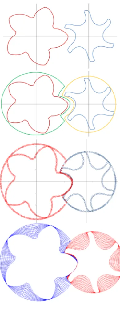
Fig. 16. Examples of a variable pitch grid with a uniform profile on 5/6 ‘N’ rotors
Approach 1 was used and three sets of grids were generated as shown in Fig. 16. In all of the grids, the node density in all the circumferential, radial and axial directions was maintained the
same. The first grid is with a uniform pitch, the second is with a linear pitch variation such that
the starting pitch is the same as that of the uniform rotors but it ends with a low pitch of 20.00
mm. This variation gives an increased wrap angle of 425°. The third example is where the initial
pitch is high at 80.00 mm and the final pitch is low at 20.00 mm. This variation gives a wrap
angle of 340°, close to the uniform pitch rotors. The examples shown for variable pitch in Fig. 16
are to demonstrate the grid generation capability although this high level of variation may not be
18 4.4 Grid Generation examples for uniform pitch and variable profile
As an example of grid generation with uniform pitch and variable section, a 3/5 lobe
combination compressor with ‘Rotor Generated N’ profiles was generated. The original rotor
design was with an L/D ratio of 1.7, wrap angle of 306° and a rotor length of 230.775 mm.
Fig. 17. Example of a uniform pitch grid with a variable profile on 3/5 ‘Rotor Generated N’ rotors
Approach 2 was used and a set of grids was generated as shown in Fig. 17. In all of the grid sections, the node density in all the circumferential, radial and axial directions was maintained
the same. The cross sections changes continuously from suction end to the discharge end of the
rotors. As the centre distance is fixed, the rotors are of parallel axis and a tapered shape. The
outer diameter on the main rotor is tapered while the inner diameter is constant while on the gate
rotor, the inner diameter is tapered and the outer is constant.
Fig. 18. Grid sections of variable geometry on 3/5 ‘Rotor Generated N’ rotors
Fig. 18 shows the 2D cross sections grids for variable rotor profile at the suction end, middle of
the rotors and the discharge end.
5 CFD Analysis
The numerical analysis was carried out with the objective of validating the new grid generation
procedures and to study the flow behaviour in variable geometry screw compressors.
The test case is an oil free twin screw compressor. Male rotor has 3 lobes with 127.45mm outer
19 to rotor centre distance is 93mm. Rotors are rack generated ‘N’ profiles. The compressor speed is
8000 rpm with pressure ratio of 2.0 and 3.0. Four test cases were calculated.
Case 1. Uniform pitch and uniform profile rotors with built in volume index Vi of
1.8.
Case 2. Uniform Pitch and Profile rotors with a reduced discharge port opening area to give a built in volume index Vi of 2.2. In this case, the compression chamber is exposed
to the discharge pressure relatively late in the cycle as shown in Fig. 19 and allows for further
pressure build up in the chambers.
Fig. 19. Reduced discharge port area in Case 2 compared with Case 1
Case 3. Variable pitch with uniform profile rotors and built in volume index Vi >
1.8. The Suction side pitch was 130mm and Discharge side pitch was 40mm. The wrap angle of
Φw 285° was maintained as shown in Fig. 20.
Fig. 20. Variable pitch grid – 3/5 ‘N’ rotors
Case 4. Variable profile and uniform pitch rotors. Rotor profile in successive sections is generated using rack generation procedure by variation of addendum on the defining
racks [28]. Addendum on the suction end of the rotors was 33mm while on the discharge side it
was reduced to 21mm. The addendum on the uniform profile rotors had constant value
28.848mm. Due to the variation of addendum the outer diameter of the male rotor is changing
while the inner diameter remains constant and vice versa for the female rotor as shown in Fig.
21. The displacement of these rotors is smaller than for the uniform profile rotors.
20 Each rotor configuration was analysed on three levels of successive grid refinements. Table 1
shows the number of computational nodes in each case. Stationary compressor ports were
meshed by use of the commercial grid generator. Fig. 7 shows the different parts of the
numerical model and the grid refinement is shown in Fig. 22. The numerical solver used for the
study was ANSYS CFX [1], which uses a vertex-based Finite Volume Method and iteratively solves for momentum and continuity in a pressure coupled algorithm. All the generated grids are
passed to the solver in the model setup and during solution the rotor domain grids were updated
for every time step using external subroutines. The space conservation law is retained during this
grid motion by modifications to the governing equation as described by Ferziger and Peric in [4]. The solver was set with a Higher Order advection scheme and a Second Order Backward Euler temporal discretization.
Fig. 22. Different level of grid refinements shown for one section
Table 1. Grid refinement as number of computational nodes
The boundary conditions at the suction and discharge of the compressor are highly unsteady and
therefore difficult to specify. To provide good boundary conditions, the ports were reasonably
extended to get good convergence of the flow and reduce the numerical discrepancies arising
from pressure pulses in the flow. The working gas was air with an equation of state defined by
the Ideal gas law for density. The suction receiver pressure was 1.0bar absolute and the
Discharge receiver pressure was 2.0bar and 3.0bar absolute. The convergence criteria for all
equations were targeted at 1.0x10⁻³ and the coefficient loops for every time step were set at 10.
During the solution, the rms residuals for all the time steps were between 1.0x10⁻³ and 5.0x10⁻³
21 calculations were run until cyclic repetition of the flow and pressure characteristics were
identified at the boundaries. Each case was calculated with both Laminar and SST k-Omega
Turbulence model.
5.1 Results and Discussion
5.1.1 Compression characteristics
Fig. 23 shows the variation of pressure in case of variable pitch rotors. Fig. 24 shows the
compression characteristic of cases 1, 3 and 4 for one full cycle on fine grids with discharge
pressure of 2.0bar. With uniform rotors the maximum internal pressure goes up to 2.5bar and
with variable geometry rotors the maximum internal pressure goes up to 3.0bar. Case 3 with the variable rotor pitch and Case 4 with variable rotor profile have a steeper rise in internal pressure than Case 1 which has constant rotor geometry. The highest peak pressure is achieved with the variable pitch rotors. For a discharge pressure of 2.0bar this internal pressure rise is a condition
of over-compression.
Fig. 23. Pressure variation on variable pitch medium grid case with discharge pressure 2.0bar.
Fig. 24. Indicator diagram for cases calculated on fine grid. Discharge pressure 2.0 bar.
Fig. 25 shows the compression characteristic of the four cases on fine grids with discharge pressure of 2.0bar and 3.0bar and SST k-omega turbulence models. Uniform rotors show high under compression and with variable geometry rotors the maximum pressure goes up to 3.4bar.
Fig. 25. Indicator diagram for cases calculated on fine grid with turbulence models. Discharge pressure
2.0bar and 3.0 bar.
5.1.2 Discharge Port Area
Fig. 19 shows a decrease in the discharge port area with the increased Vi to 2.2. In Case 2, with
22 3.1bar before exposure to a discharge pressure of 2.0bar as seen in Fig. 25. This pressure rise
was close to that of the variable geometry rotors of about 3.0bar, for which the opening area was
22% higher. The increment in the discharge area for comparable pressure rise is favourable to the
reduction of throttling losses in the compressor.
5.1.3 Influence of grid refinement
Fig. 26 shows the effect of grid refinement on the prediction of integral quantities such as the mass flow rate, indicated power and specific power for cases 1, 3 and 4 with 2.0bar discharge pressure. The mass flow rate showed an increase with grid refinement in all cases. The difference between each consecutive grid refinement is around 10%.
Fig. 26. Effect of grid refinement on integral parameters in cases 1,3 and 4 with 2.0bar discharge pressure
This indicates that the rotor geometry is captured better with finer grids, which results in reduction of leakages. Similarly, indicated power increases by 2-5% each time the grid is refined. The increase in the chamber pressure with grid refinement is shown in Fig. 27 for the Case 4
with variable profile rotors as an example.
Fig. 27. Indicator diagram for cases 4 showing effect of grid refinement with 2.0bar discharge pressure
5.1.4 Influence of Turbulence Model
As shown in Fig. 26, higher mass flow rates are achieved when the turbulence model is applied.
Indicated power also increases as the consequence of increased mass flow. However, specific
power is reduced for all turbulent cases indicating that influence of turbulence models on mass
flow rate prediction is higher than that on indicator diagram/power prediction.
5.1.5 Sealing Line Length
The interlobe sealing line is the line of closest proximity between the two rotors. The leakage of
gas takes place through this gap and is proportional to the length of the sealing line and clearance
23 numerical calculations and the dividing line between high and low pressure levels can be
considered as the sealing line. The maximum pressure gradient is present across this division and
is the driving force for leakage.
Fig. 28. Comparison of interlobe sealing line lengths
Fig. 28 shows the sealing lines obtained on the uniform pitch rotors (Case 1) and variable geometry rotors (Case 3 and Case 4). The projection of the sealing line on the rotor normal plane shows the difference more clearly. The sealing line on the uniform pitch rotor is of the same
length for each interlobe space along the rotor. However, on the variable pitch rotors the sealing
line is longer at the suction end. It decreases towards the discharge end of the rotor.
Table 2. Comparison of Interlobe Sealing Line Length [mm]
Table 2 presents the variation in the sealing line lengths between the uniform and variable
geometry cases at one of the rotor positions indicating the magnitude of change along the rotors.
At the suction end the sealing line on variable pitch rotor is 30mm longer but at the discharge
end it is 12mm shorter. This helps to reduce leakage as the largest pressure difference across the
sealing line is at the discharge. Additionally, the total length of the sealing line is reduced by
11mm in the variable pitch rotors. In Case 4 with variable profile the suction end is longer by 12mm and discharge end has very small difference compared with the uniform profile. There is
no overall gain in sealing line length because of the increased gate lobe thickness near the
discharge end of the rotors.
5.1.6 Blow-hole area
Blow-hole area is the leakage area formed between the male and female rotors and the casing at
24 leakage due to the pressure difference between adjacent compression chambers. A smaller
blow-hole area is desired for improved performance of the machine. Table 3 shows the blow-blow-hole
areas measured on the medium size grid for different calculated cases at three positions on the
rotor.
Fig. 29. Comparison of Blow-hole area
Table 3. Comparison of Blow-hole area [mm2]
The blow-hole area for the uniform rotors remains constant along the length of the rotors. In the
variable pitch rotors, the suction side blow-hole area is larger than in the uniform rotors but the
discharge side blow-hole area is smaller than for the uniform rotors. In the variable profile rotors,
the suction side blow-hole area is nearly the same as that of the uniform rotors but the discharge
blow-hole area is smaller than for the uniform rotors. Proportionally, the reduction of blow-hole
area towards the discharge side rotors is most pronounced in the case of variable pitch rotors.
5.1.7 Overall performance
The influence of the discharge pressure on the compressor performance for the analysed cases 1,
3 and 4 is shown in Fig. 30. Uniform rotors have a highest flow rate and lowest specific power
for both pressures. However the difference in the specific power between uniform and variable
geometry rotors is much reduced at higher pressures.
Fig. 30. Comparison of performance at 2.0bar and 3.0bar discharge pressure with fine grid cases
Table 4. Comparison of predicted variable geometry rotor efficiencies
Table 4 shows the comparison of predicted volumetric and adiabatic efficiencies. Uniform rotors
show highest volumetric efficiency at 2.0bar. But with Vi 2.2 the efficiency is lower than that of
25 line length in variable pitch rotor. Also variable pitch rotors have higher volumetric efficiency at
3.0bar discharge pressure.
Uniform rotors show highest adiabatic efficiency at 2.0bar. But with Vi 2.2 the efficiency is
lower than that of variable geometry rotors. At 3.0 bar discharge pressure variable geometry
rotors have equivalent adiabatic efficiency with uniform rotors and higher than their efficiencies
at 2.0 bar discharge pressure due to reduced over-compression losses at 3.0bar discharge
pressure. This further supports that the variable pitch rotors are more suitable for high pressure
applications.
Variable profile rotors show lower volumetric efficiency as compared to uniform rotors due to
smaller capacity of the machine and also higher internal pressure rise. The over-compression
before discharge results in lower adiabatic efficiency except at 3.0bar discharge pressure where it
is comparable with uniform rotors.
6 Conclusion
3D CFD grid generation for twin screw compressors with variable pitch and variable profile
rotors was formulated and implemented. Examples of grids with variable geometries have been
presented and CFD analysis has shown the flow characteristics in the machines.
From the numerical analysis presented here, flow advantages identified with variable geometry
rotors were evaluated. The analysis showed that by varying the rotor lead continuously from the
suction to the discharge ends, it is possible to improve compression characteristics with a steeper
internal pressure build up. The analysis also showed that varying the rotor lead allows a larger
size of discharge port area, thereby reducing throttling losses, and provides increase in
volumetric efficiency by reducing the sealing line length in the high pressure zone. Analysis of
26 sealing line length and blow-hole area with this size of the rotors. The increase in root diameter
of the female rotors with variable profile certainly helps in producing stiff rotors for high
pressure applications.
These grid generation developments open new opportunities for further investigation of the flow
27 References
1. ANSYS 13.0, User Guide and Help Manual, 2011.
2. P.R. Eiseman, Control Point Grid Generation, Computers & Mathematics with Applications, 1992; 24, No.5/6, 57-67.
3. P.R. Eiseman, J. Hauser, J.F. Thompson and N.P. Weatherill, Numerical Grid Generation
in Computational Field Simulation and Related Fields, Proceedings of the 4th International Conference, Pineridge Press, Swansea, Wales, UK, 1994.
4. J.H. Ferziger and M. Peric, Computational Methods for Fluid Dynamics, ISBN
978-3-540-42074-3, Springer, Berlin, Germany, 1996.
5. J.S. Fleming and Y. Tang, The Analysis of Leakage in a Twin Screw Compressor and its
Application to Performance Improvement, Proceedings of IMechE, Part E, Journal of Process Mechanical Engineering, 1994; 209, 125.
6. J.S. Fleming, Y. Tang and G. Cook, The Twin Helical Screw Compressor, Part 1: Development, Applications and Competitive Position, Part 2: A Mathematical Model of the Working process, Proc. Inst. Mech. Eng. Part C J. Mech. Eng. Sci., 1998; 212, 369. 7. J.W. Gardner, US Patent No 3,424,373 – Variable Lead Compressor. Patented 1969.
8. K. Hanjalic and N. Stosic, Development and Optimization of Screw machines with a
simulation Model – Part II: Thermodynamic Performance Simulation and Design
Optimization. ASME Transactions. Journal of Fluids Engineering. 1997; 119, 664.
9. J.H. Kim and J.F. Thompson, Three-Dimensional Adaptive Grid generation on a
28 10.A. Kovacevic, N. Stosic and I.K. Smith, Development of CAD-CFD Interface for Screw
Compressor Design, International Conference on Compressors and Their Systems, London, IMechE Proceedings, 1999; 757.
11.A. Kovacevic, N. Stosic and I.K. Smith, Grid Aspects of Screw Compressor Flow
Calculations, Proceedings of the ASME Advanced Energy Systems Division, 2000; 40, 83. 12.A. Kovacevic, Three-Dimensional Numerical Analysis for Flow Prediction in Positive
Displacement Screw Machines, Ph.D. Thesis, School of Engineering and Mathematical
Sciences, City University London, UK, 2002.
13.A. Kovacevic, N. Stosic and I.K. Smith, Numerical Simulation of Fluid Flow and Solid
Structure in Screw Compressors, Proceedings of ASME Congress, New Orleans, IMECE
2002; 33367.
14.A. Kovacevic, N. Stosic and I.K. Smith, 3-D Numerical Analysis of Screw Compressor
Performance, Journal of Computational Methods in Sciences and Engineering, 2003; 3, 2, 259-284.
15.A. Kovacevic, N. Stosic and I.K. Smith, A numerical study of fluid–solid interaction in
screw compressors. International Journal of Computer Applications in Technology. 2004; 21, 4, 148 – 158.
16.A. Kovacevic, Boundary Adaptation in Grid Generation for CFD Analysis of Screw
Compressors, Int. J. Numer. Methods Eng., 2005; 64, 3, 401-426.
17.A. Kovacevic, N. Stosic and I.K. Smith, Numerical simulation of combined screw
29 18.A. Kovacevic, N. Stosic and I.K. Smith. Screw compressors - Three dimensional
computational fluid dynamics and solid fluid interaction, ISBN 3-540-36302-5, Springer-Verlag Berlin Heidelberg New York, 2007.
19.V.D. Liseikin, Algebraic Adaptation Based on Stretching Functions, Russian Journal for Numerical and Analytical Mathematical Modeling, 1998; 13, 4, 307-324.
20.V.D. Liseikin, Grid Generation Methods, ISBN 3-540-65686-3, Springer-Verlag (1999).
21.B.G. Prasad, CFD for Positive Displacement Compressors, Proc. Int. Compressor Conf. at Purdue. 2004; 1689.
22.S. Rane, A. Kovacevic, N. Stosic and M. Kethidi, Grid Deformation Strategies for CFD Analysis of Screw Compressors, Int Journal of Refrigeration, http://dx.doi.org /10.1016/j.ijrefrig.2013.04.008, 2013.
23.A.J. Samareh and R.E. Smith, A Practical Approach to Algebraic Grid Adaptation,
Computers & Mathematics with Applications, 1992; 24, 5/6, 69-81.
24.T.I.P. Shih, R.T. Bailey, H.L. Ngoyen and R.J. Roelke, Algebraic Grid Generation For
Complex Geometries, Int. J. Numer. Meth. Fluids, 1991; 13, 1-31.
25.B.K. Soni, Grid Generation for Internal Flow Configurations, Computers & Mathematics with Applications, 1992; 24, 5/6, 191-201.
26.E. Steinthorsson, T.I.P. Shih and R.J. Roelke, Enhancing Control of Grid Distribution In
Algebraic Grid Generation, Int. J. Numer. Meth. Fluids, 1992; 15, 297-311.
27.N. Stosic, On Gearing of Helical Screw Compressor Rotors, Journal of Mechanical Engineering Science, 1998; 212, 587.
30 29.J.F. Thompson, Grid Generation Techniques in Computational fluid Dynamics, AIAA
Journal, 1984; 22, 11, 1505-1523.
30.J.F. Thompson and B. Soni, Weatherill NP. Handbook of Grid generation, CRC Press,
1999.
31.J.V. Voorde, J. Vierendeels and E. Dick, Development of a Laplacian-based mesh
generator for ALE calculations in rotary volumetric pumps and compressors. Computer Methods in Applied Mechanics and Engineering, 2004; 193, 39–41, 4401-4415.
32.J.V. Voorde and J. Vierendeels, A grid manipulation algorithm for ALE calculations in
31 Figure Captions
Fig. 1. Oil free Twin Screw compressor and its working chamber
Fig. 2. Meshing of Uniform Pitch Twin Screw Rotors
Fig. 3. Meshing of Variable Pitch Twin Screw Rotors
Fig. 4. Volume-Angle diagram
Fig. 5. Pressure-Angle Diagram
Fig. 6. Cylinder and Port development of a rotor pair
Fig. 7. Twin screw compressor working chamber domains
Fig. 8. Simplified Block Diagram of Screw Compressor Rotor Grid Generator
Fig. 9. Uniform Pitch Grid Generation
Fig. 10. Uniform Pitch Rotor Grid Assembly in 3D
Fig. 11. Axial spacing difference between uniform pitch and variable pitch rotor grids
Fig. 12. Globoid type single screw compressor rotor with variable section profile
Fig. 13. Angular rotation of sections for different Pitch Functions
Fig. 14. Variable Pitch and Variable Profile Grid Generation
Fig. 15. Grid Assembly in 3D for Variable Pitch and Variable Profile rotors
Fig. 16. Examples of variable pitch grid with uniform profile on 5/6 ‘N’ rotors
Fig. 17. Example of a uniform pitch grid with a variable profile on 3/5 ‘Rotor Generated N’
rotors
Fig. 18. Grid sections of variable geometry on 3/5 ‘Rotor Generated N’ rotors
Fig. 19. Reduced discharge port area in Case 2 compared with Case 1
Fig. 20. Variable pitch grid – 3/5 ‘N’ rotors
32 Fig. 22. Different level of grid refinements shown for one section
Fig. 23. Pressure variation on variable pitch medium grid case with discharge pressure 2.0bar.
Fig. 24. Indicator diagram for cases calculated on fine grid. Discharge pressure 2.0 bar.
Fig. 25. Indicator diagram for cases calculated on fine grid with turbulence models. Discharge
pressure 2.0bar and 3.0bar
Fig. 26. Effect of grid refinement on integral parameters in cases 1,3 and 4 with 2.0bar discharge
pressure
Fig. 27. Indicator diagram for cases 4 showing effect of grid refinement with 2.0bar discharge
pressure
Fig. 28. Comparison of Interlobe Sealing Line Lengths
Fig. 29. Comparison of Blow-hole area
33
Deforming Grid Generation and CFD analysis of Variable
Geometry Screw Compressors
[image:34.612.135.484.202.458.2]Sham Rane*, Ahmed Kovacevic, Nikola Stosic, Madhulika Kethidi
56 Fig. 24. Indicator diagram for cases calculated on fine grid. Discharge pressure 2.0 bar.
Fig. 25. Indicator diagram for cases calculated on fine grid with turbulence models. Discharge
63 Table 1 Grid refinement as number of computational nodes
Case Uniform Variable Pitch
Variable Profile
Coarse 691174 648190 675918
Medium 838378 915184 889794
Fine 1214418 1344944 1297434
Table 2 Comparison of Interlobe Sealing Line Length [mm]
Interlobe
No Uniform
Variable
Pitch Difference
Var.
Prof Difference
1 145.8 175.9 -30.1 158.4 -12.6
2 170.3 164.0 +6.4 162.2 +08.1
3 (part) 069.1 056.8 +12.2 068.4 +00.6
Total 385.2 396.6 -11.5 389.1 -03.9
Table 3 Comparison of Blow-hole area [mm2]
Position Uniform Var.
Pitch Diff %
Var.
Profile Diff %
Suction 9.817 12.49 -27.2 9.83 -0.15
Mid 9.908 9.263 6.51 9.35 5.64
Discharge 9.701 6.562 32.3 9.19 5.29
Table 4 Comparison of predicted variable geometry rotor efficiencies
Volumetric
Efficiency %
Adiabatic
Efficiency %
2.0 bar 3.0 bar 2.0 bar 3.0 bar
[image:64.612.87.530.627.720.2]64
Uniform Vi 2.2 64.00 55.66 44.06 49.91
Variable Pitch
Vi > 1.8 66.20 57.60 46.88 50.99
Variable Profile