Ultimate iterative UFIR filtering algorithm

(1)

City, University of London Institutional Repository

Citation

:

Shmaliy, Y. S., Khan, S. and Zhao, S. (2016). Ultimate iterative UFIR filtering

algorithm. Measurement, 92, pp. 236-242. doi: 10.1016/j.measurement.2016.06.029

This is the accepted version of the paper.

This version of the publication may differ from the final published

version.

Permanent repository link: http://openaccess.city.ac.uk/15831/

Link to published version

:

http://dx.doi.org/10.1016/j.measurement.2016.06.029

Copyright and reuse:

City Research Online aims to make research

outputs of City, University of London available to a wider audience.

Copyright and Moral Rights remain with the author(s) and/or copyright

holders. URLs from City Research Online may be freely distributed and

linked to.

City Research Online:

http://openaccess.city.ac.uk/

[email protected]

(2)

Ultimate iterative UFIR filtering algorithm

Yuriy S. Shmaliy

a,_⇑

_{, Sanowar Khan}

b

_{, Shunyi Zhao}

c a_{Department of Electronics Engineering, Universidad de Guanajuato, 36885 Salamanca, Mexico} b_{Department of Electronics Engineering, City University London, London, UK}

c_{Key Laboratory of Advanced Process Control for Light Industry, Jiangnan University, Wuxi, China}

a r t i c l e i n f o

Article history: Received 18 March 2016

Received in revised form 27 May 2016 Accepted 13 June 2016

Available online 15 June 2016

Keywords: Unbiased FIR filter Kalman filter Noisy measurements State estimation

a b s t r a c t

Measurements are often provided in the presence of noise and uncertainties that require optimal filters to estimate processes with highest accuracy. The ultimate iterative unbiased finite impulse response (UFIR) filtering algorithm presented in this paper is more robust in real world than the Kalman filter. It com-pletely ignores the noise statistics and initial values while demonstrating better accuracy under the mis-modeling and temporary uncertainties and lower sensitivity to errors in the noise statistics.

1. Introduction

Optimal estimation of system state is often required when mea-surements are provided in the presence of noise. If the process and its measurement are both linear and noise is white Gaussian, then the Kalman filter (KF) is recognized to be the best estimator. How-ever, real life dictates that the conditions cannot always be satis-fied for the KF. Therefore, it may produce extra errors, even unacceptable. In order to improve the KF performance big efforts were made over decades. Cox in[1]has derived the extended KF (EKF) for nonlinear models by linearizing the state-space equa-tions. For highly nonlinear systems, Julier and Uhlmann employed the unscented transform[2]and proposed the unscented KF (UKF). Both EKF and UKF have then been used extensively. In[3], the EKF was developed to the invariant EKF for nonlinear systems possess-ing symmetries (or invariances). For high-dimensional systems, the ensemble KF was proposed by Evensen in[4]and, for systems with sparse matrices, the fast KF applied by Lange in[5]. The robust Kal-man filter was designed by Masreliez[6,7]for linear state-space relations with non-Gaussian noise referred to as heavy tailed noise or Gaussian one mixed with outliers. Essential contributions to robust and highly robust estimation were also made in [8–10]. Most recently, Li et al. have developed in[11]an advanced robust unscented KF with an adaptive ability to changes in noise covariances.

Many other modifications have also attracted researches atten-tion, just a few to mention. An efficient restoration Kalman-like algorithm was designed by Basseville et al. in[12]for hidden Mar-kov trees. In[13], the KF was developed by Soken et al. for the con-ditions of small satellite attitude estimation with missed measurements. Ait-El-Fquih and Desbouvries applied in[14] the Kalman-like approach to triple Markov chains. Kalman filtering was also developed by Vaswani in [15]and Carmi et al. in[16] for sparse signals with unknown and time-varying sparsity pat-terns. An efficient Kalman-like tracking algorithm[17]was applied to the autoregressive channel process estimation with fading by Stefanatos and Katsaggelos. In [18], Becis-Aubry et al. discussed the two-step estimation algorithm with a switching gain matrix. In[19], Carli et al. employed the concept of the centralized KF for state estimation in the complex wireless sensor networks. Rawicz et al. reported in[20]explicit Kalman–Bucy-like solutions for two-state H1and H2filters. In[21], Jwo and Cho have made several

use-ful remarks regarding the linearized and extended Kalman filters, and we meet new useful solutions each year.

Notwithstanding the fact that the KF is definitely the best linear real-time estimator and in spite of a number of its essential improvements, the KF still may suffer of unacceptable errors when the model does not match the system exactly, the process implies uncertainties, noise is not white Gaussian, and the noise statistics are defined imprecisely. Jazwinski has resumed in[22]that poor performance of the KF in real world has a lot to do with its infinite impulse response[22]and that finite impulse response (FIR) filter-ing is more successful in accuracy under the real-world conditions. He also formulated the key motivation to develop FIR filters:

⇑Corresponding author.

E-mail address:[email protected](Y.S. Shmaliy).

Contents lists available atScienceDirect

Measurement

(3)

A limited memory filter appears to be the only device for preventing divergence in the presence of unbounded perturbation in the system. That means that the FIR filter is inherently more robust than the IIR (Kalman) filter as it does not project ‘‘old” errors to the esti-mate. In the subsequent decades, FIR filtering has been investi-gated profoundly to offer several important solutions. Kwon and Han have developed the theory of the bias-constrained receding horizon (one-step predictive) control[23]utilizing measurement data from the horizon½k"N;k"1#, wherekis the current discrete

time index andNis the horizon length. Diverse receding horizon FIR solutions were proposed in[24–28]. Shmaliy et al. have devel-oped FIR filtering on the horizon½k"Nþ1;k#that has resulted in several optimal, unbiased, and in-between solutions[29–33]. Most recently, receding horizon FIR filtering has been developed by Ahn et al. in[34–38]and Zhao et al. have found fast iterative forms for FIR filters in[39,40].

Among different kinds of FIR filters developed during decades, the unbiased FIR (UFIR) filter is most robust. This filter [32,28] appears as a solution to the unbiasedness constraint[24]or as a special case of the optimal FIR (OFIR) filter[30]when the model is noiseless. The UFIR filter has the embedded bounded input/ bounded output (BIBO) stability and its algorithm completely ignores the noise statistics and initial conditions. The UFIR filter does not guarantee optimality, but the variance of its estimate diminishes as a reciprocal of the averaging horizon ofN points. Accordingly, it becomes practically optimal whenN%1 and this

is in agreement with the Gauss’s ordinarily least squares (OLS). Advantages of the iterative UFIR algorithm go along with the requirements of the optimal horizon ofNoptpoints which is applied

to minimize the mean square error (MSE). Of practical importance is that a single tuning factorNoptcan be determined in a way much

easier than for the noise statistics: using reference measurements or even via observations without a reference model[31]. The bad side is that iterations require aboutNopttimes more computation

time and this price paid for the advantages may be an issue in real-time applications. But using parallel computing can make the UFIR algorithm as fast as the KF.

Although diverse forms of the UFIR filter have been discussed in many papers[32,33,41–43], its most demanded linear algorithm still has not been addressed to the engineer in a simple form. In this technical note, we introduce the ultimate iterative UFIR filter-ing algorithm suitable for immediate use.

2. Measured process and estimates

A big class of engineering problems can be solved if to represent the process and its measurement with the K-state space linear model as

xk¼Fkxk"1þwk; ð1Þ

yk¼Hkxkþ

v

k; ð2Þ

wherexk2RKis the system state vector,Fk2RK)Kis the state

tran-sition matrix,yk2RMis the observation vector, andHk2RM)K is

the measurement matrix. The process noise wk2RK*Nð0;QkÞ

and the observation noise

vk

2RM*Nð0;RkÞare both zero mean

and white Gaussian with covariances,QkandRk. Vectorswkand

vk

and the initial state are uncorrelated and independent at each time step. For our purposes, we assignx^kjrto be an estimate ofxk

at time-indexkvia measurements from past up to and including at time-indexr. We will also employ the following variables:

^ x"

k ,^xkjk"1, thea priori(prior or predicted) state estimate given

observations up to and including at timek"1;

P"

k,Pkjk"1¼Efðxk"^x"kÞðxk"^x"kÞ T

g, thea priori (prior or pre-dicted) estimate covariance given observations up to and including at timek"1;

^

xk,^xkjk, thea posteriorior posterior state estimate given

obser-vations up to and including atk;

Pk,Pkjk¼Efðxk"x^kÞðxk"^xkÞTg, the a posteriori or posterior

error covariance matrix given observations up to and including atk.

The KF applied to(1) and (2)produces estimates recursively in one step and is the best optimal engineering solution among other known real-time estimators. It is also simple in programming. But, in order for the KF estimate to be optimal, the initialx0andP0as

well as the noise covariances,QkandRk, must be given that is

typ-ically not the case in practice. Experience dictates that the imple-mentation of optimal KF is difficult due to the inability in getting good estimates of these values and the KF is thus suboptimal for all practical purposes.

2.1. Unbiased FIR filtering estimate

In contrast to the KF, the UFIR filter operates at once withN

measurements on a horizon from m¼k"Nþ1 to k and does not require neither the initial statexmand errorPmnor the noise

statisticsQiandRi; i2½m;k#. Instead it claims thatNmust be

opti-mal,Nopt, in order to minimize the MSE and produce near optimal

estimate. To run the iterations, the UFIR algorithm self determines the statex^mþK"1atmþK"1 in a short batch form, whereKis the

number of the system states. It then updates estimates iteratively using recursions to reach the best value at k. The estimate x^k

obtained in such a way is called in[33]the optimal UFIR (OUFIR) estimate. Note that the estimation error covariance Pk is not

involved to the algorithm that is an important advantage against the KF.

2.1.1. Batch UFIR estimate

The cost function for the UFIR filter is the unbiasedness condition

Ef^xkg¼Efxkg; ð3Þ

which means that the average of the state estimate is required to be equal to the average of the state. In the OLS format, the UFIR esti-mate can be written on a horizon½m;k#as[30]

^

xk¼ ðCTm;kCm;kÞ"

1

CT

m;kYm;k; ð4Þ

where the extended observation vector Ym;kand mapping matrix Cm;kare represented as

Ym;k¼ yTmyTmþ1. . .yTk

! "T

; ð5Þ

Cm;k¼

HmðFmkþ1Þ "1

Hmþ1ðFmkþ2Þ "1

.. .

Hk"1F"k1 Hk 2 6 6 6 6 6 6 6 6 4

3 7 7 7 7 7 7 7 7 5

; ð6Þ

and the product of system matrices is depicted as

Frg¼

FrFr"1. . .Fg; g6r;

I; g¼rþ1

0; otherwise: 8

> < >

: ; ð7Þ

(4)

^

xk¼Km;kYm;k; ð8Þ

whereKm;kis theUFIR filter gaingiven by

Km;k¼ ðCTm;kCm;kÞ"1CTm;k ð9Þ

¼GkCTm;k: ð10Þ

MatrixGkis known as thegeneralized noise power gain(GNPG) [44]computed as

Gk¼Km;kKTm;k ¼ ðCT

m;kCm;kÞ"

1

: ð11Þ

The GNPG plays an important role in FIR filtering. It originates from the noise power gain (NPG) introduced by Trench in[45]as a ratio of the FIR filter output noise variance

r

2

outto the input noise

variance

r

2

in. As such, the NPG is akin to the noise figure in wireless

communications. Trench has also shown that the NPG for white Gaussian noise is equal to the sum of the squared coefficients of the FIR filter impulse response functionhðkÞ,

NPG¼

r

2 out

r

2 in ¼ X N"1 n¼0

h2ðkÞ; ð12Þ

which is the squared norm ofhðnÞ. In state space,Km;krepresents

coefficients of the filter impulse response. Therefore, Km;kKTm;k is

called the GNPG.

2.1.2. Iterative UFIR estimate

The fast iterative form for(4)was found in[32]. Below, we give a more simple derivation to the iterative UFIR filtering algorithm.

Consider (4) and represent the inverse of the GNPG

Gk¼ ðCTm;kCm;kÞ"

1

as

G"1

k ¼CTm;kCm;k

¼X

N"1

i¼0

ðFmþ1þi

k Þ

"T HT

mþiHmþiðFmkþ1þiÞ

"1 ð13Þ

¼HT

kHkþ X N"2

i¼0

ðFmþ1þi

k Þ

"T HT

mþiHmþiðFmkþ1þiÞ "1

¼HT

kHkþF"kT X N"2

i¼0

ðFmþk"11þiÞ

"T HT

mþiHmþiðFmþk"11þiÞ

"1

" #

F"1

k :

ð14Þ

From(7), we haveFrg¼0 ifg>rþ1 and one can findG"k"11

from(13)as

G"1

k"1¼

XN"2

i¼0

ðFmþk"11þiÞ

"T HT

mþiHmþiðFmþk"11þiÞ

"1

ð15Þ

that is exactly the term in brackets of(14). By combining(14) and (15), we arrive at the recursion for the GNPG,

Gk¼ ½HTkHkþ ðFkGk"1FTÞ" 1

#"1: ð16Þ

Similarly, represent the productCT m;kYm;kas

CT

m;kYm;k¼HTkykþF"Tk XN"2

i¼0

ðFmþk"11þiÞ

"T Hmþiymþi

¼HTkykþFk"TCTm;k"1Ym;k"1:

ð17Þ

Combine(4)with(17)and write

^

xk¼GkðHTkykþFk"TCTm;k"1Ym;k"1Þ: ð18Þ

From(4)taken atk"1 findCT

m;k"1Ym;k"1¼G"k"11^xk"1and go from

(18)to

^

xk¼GkðHTkykþF"Tk G"k"11^xk"1Þ: ð19Þ

By simple manipulations with (16), find

G"1

k"1¼FTkðG"k1"HTkHkÞFk, substitute into(19), provide the

transfor-mations, and arrive at the recursive Kalman-like form of[32],

^

xk¼Fk^xk"1þKkðyk"HkFk^xk"1Þ; ð20Þ

in whichKk¼GkHTkis the bias correction gain that is not the

Kal-man gain and the GNPGGkis computed recursively by(16).

As well as in the KF, each recursion in the UFIR filter implies two phases: ‘‘Predict” and ‘‘Update”. Following the UFIR filter strategy, the estimate at time-indexkis obtained iteratively with an auxil-iary variablelbeginning withl¼mþKand ending whenl¼k. To run iterations, the initial estimate at l¼mþK"1 is provided

using (4) in a shortest available batch form on a horizon

½m;mþK"1#, because the inverse in(4)does not exist otherwise.

Since the UFIR algorithm does not require the noise statistics, the predict phase computes only one value – thea prioristate esti-mate^x"

l ¼Fl^xl"1. Combined with the current state observation to

refine the state estimate, thea prioristate estimate is iteratively updated to thea posterioristate estimate via the following values: the GNPG(16), the measurement residualzl¼yl"Hl^x"l, the bias

correction gainKl¼GlHTl, which is not the Kalman gain, and the

a posterioristate estimatex^l¼x^"l þKlzl.

The iterative UFIR filtering algorithm is given inTable 1with a pseudo code. The only tuning parameter required by this algorithm is the horizon lengthNwhich must be optimal,Nopt, in order to

minimize MSE. There are at least two ways of how to find Nopt.

The value ofNoptcan be ascertained at the early stage by

minimiz-ing the trace of the estimation error covariancePkas

Nopt¼arg min

N ftrPðNÞg: ð21Þ

In this case, the system statexkis measured using test

equip-ment and supposed to be known. Otherwise,Noptcan be estimated

via measurementykwith no reference as shown in[31]:

Noptﬃarg min

N @ @ktrLkðNÞ

# $

; ð22Þ

by minimizing the derivative of the trace of the mean square value

Lk¼Efðyk"Hkx^kÞðyk"Hkx^kÞTg:

Beyond these approaches, the correlation method was employed in [46] to find Nopt and an advanced technique was

developed in[47]to specify the minimum acceptableN. Note that, for nonlinear and time-variant systems,Noptmust be specified at

each time indexk.

Provided N, the initial values of the GNPG and estimate are computed atk"NþKand Algorithm (Table 1) produces the first estimate at N"1. Recursions are organized based on (14)–(16) and the output is taken when the iterative variable reaches the cur-rent time index,l¼k. One may thus deduce that a lack of informa-tion about noise, initial values, and error covariances is compensated in the UFIR algorithm by setting properly the GNPG which tunes the bias correction gain most closely to the Kalman gain, byNopt. Note that the minimal horizon length for the initial

(5)

2.2. Estimation errors

Even though the UFIR filter does not require the error covari-ancePkto update the estimate, the latter may be needed to

evalu-ate estimation accuracy and precision. An iterative form still has not been proposed to computePkprecisely in view of

mathemati-cal issues. But the error upper bound has a computationally simple form[33]as shown inTable 2.

ProvidedPs, recursions in this algorithm are organized with one

value in each phase. The algorithm first predicts the estimation error over the system noise covarianceQland then updates it over

the measurement noise covarianceRland the bias correction gain Kl¼GlHTl taken fromTable 1. The value produced by the algorithm

(Table 2) is overestimated for the worst case and thus an actual error should be expected to be smaller.

2.3. Properties of UFIR filter

Looking for a good estimator we naturally desire to have one that is optimal, robust, universal for different signals in diverse environments, and (!!!) simple. As well as the KF, the UFIR one is a universal linear estimator, so let us look at its ability to fulfil other requirements and measure up to optimal Kalman estimate. Before providing a comparative analysis, it is a proper place to stress again that the optimal KF is challenged by the unbiased FIR filter that is potentially lesser accurate. But this is when the operation conditions are ideal. In real world any filter falls short of the requirements in some items and the question arises of how far. The KF has the recursive IIR structure in which the feed-back plays a key role. On the contrary, the UFIR filter is a transver-sal estimator relying on the input-to-output relation with no feedback. Many properties of these estimators are due to their dif-ferent structures.

Unbiasedness vs. optimality:Unbiasedness is the necessary con-dition of any good estimate. But the unbiased estimate may suffer of extra noise because the sufficient condition – minimal variance – is not applied. In turn, the optimal estimate guarantees the min-imal MSE as a compromise between the bias and variance. Opti-mality in the KF and OFIR filter results in very consistent outputs. In turn, the UFIR filter produces a bit different and lesser precise estimate, although the difference between the unbiased and optimal estimates may practically be insignificant.

System model:The KF applies only to stochastic models. That is when bothQkandRkhave zeroth components, the KF cannot

oper-ate. In contrast, the UFIR filter serves equally well for both the stochastic and deterministic systems. Both the KF and UFIR filter have extensions to nonlinear systems in the first and second order of approximations[1,48,49]. As was observed in Section1, the KF has been extended to deal with many other practical issues. In this regard, the UFIR filter is still under the development.

Initial conditions:The UFIR filter does not require the initial con-ditions but produces the first estimate atN"1. On the contrary,

the KF requiresxkandPkatk¼0 and updates these values at each

next time step. Theory argues that there are no transients in the KF under the ideal conditions. However, transients in the KF may last much longer than in the UFIR filter in real world applications.

Noise environments:The key requirement that follows behind the derivation of the Bayesian KF estimator is that noise must be Gaussian and uncorrelated in both the state and observation equa-tions. The Kalman filter is best under such conditions provided that the noise statistics are known exactly. Otherwise, it does not guar-antee optimality. In contrast, the UFIR filter does not impose any restrictions on noise distribution and covariance and produces unbiased estimates if noise is just zero mean.

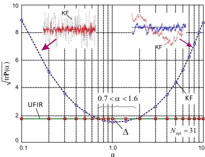
In order to produce optimal estimates, the KF requires the noise statistics at each time point. Because of this requirement and prac-tical inability to obtain good estimates ofQkandPk, the KF is

sub-optimal for all practical purposes.Fig. 1gives an idea about the KF immunity to errors in the noise statistics in the worst case. Actual covariances are substituted here withQk=

a

2 and

a

2Pk, where

a

indicates an error in the noise standard deviation. As can be seen, errors in the KF grow rapidly with

a

and may become unaccept-able, especially if a system is nonlinear[50].

In contrast, the UFIR filter ignores the noise statistics (except for the zero-mean assumption) but requires Nopt points in order to

minimize the MSE. Note thatNoptcan be measured in a way much

[image:5.595.54.294.122.259.2]

easier than for the noise statistics[31]. Furthermore, the difference

Table 1

Iterative UFIR filtering algorithm. Data:yk

Result:^xk 1:begin

2: fork¼N"1:1 do 3: m¼k"Nþ1, s¼mþK"1; 4: Gs¼ ðCT

m;sCm;sÞ"1;

5: ~xs¼GsCTm;sYm;s;

6: forl¼sþ1:k do 7: Gl¼ ½HT

lHlþ ðFlGl"1FTlÞ"

1 #"1

8: ~xl¼Fl~xl"1þGlHTlðyl"HlFl~xl"1Þ

9: end for 10: ^xk¼~xk 11: end for 12:end

Table 2

UFIR filter estimation error upper bound. Data:N;Ps;Qk,Rk;Kk,

Result:Pk 1:begin

2: fork¼N"1:1 do 3: s¼k"NþK; 4: forl¼sþ1:k do

5: Pe"

l ¼FlPel"1FTlþQl

6: Pel¼ðI"KlHlÞeP"

lðI"KlHlÞTþKlRlKTl 7: end for

8: Pbk¼ePk 9: end for 10:end

0.1 1.0 10

0 2 4 6 8 10

α

KF UFIR 0.7 1.6

31 opt

N

)

(

tr

P

KF

[image:5.595.328.533.572.729.2]

(6)

between the optimal and unbiased estimates becomes negligible if

Nopt%1. This means that, invoking no information about noise,

the UFIR filter is able to produce virtually optimal estimates.

Robustness:Two issues require robustness from an estimator. The model may not match a process accurately that causes mis-modeling errors. Temporary uncertainties in the process and mea-surements may also lead to errors. Fig. 2 illustrates typical responses of the KF and UFIR filter to temporary uncertainties in the 2-state polynomial model. As can be seen, under the ideal con-ditions (

a

¼1) both filters act quite similarly, except that the KF

may have lasting transients owing to IIR. A situation changes dra-matically if to admit errors in the noise statistics with

a

>1. In this case, the KF falls very short of the UFIR filter and its performance becomes particularly poor. An overall conclusion that can be made is that in real world the UFIR filter may demonstrate much better robustness than KF.

Stability:Both the KF and UFIR filter are stable filters but the transversal UFIR filter structure has the imbedded BIBO stability. For linear systems, neither the KF nor UFIR filter can pretend to be essentially advantageous in this plane under the ideal condi-tions. For nonlinear systems, extended versions of both these filters become unstable close to borders of high nonlinearities. It has also been observed in many nonlinear systems that the KF is more stable under the ideal conditions and it loses to the UFIR filter and may even diverge otherwise.

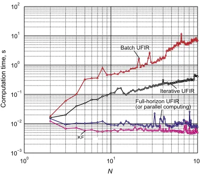
Computational complexity:Any digital estimator links its com-putation time directly to the comcom-putational complexity. From this standpoint, the KF has the lowest complexityOð1Þand is the fastest one. The full-horizon UFIR algorithm [30,33] which iteratively updates the estimate over all time also has low complexityOð1Þ

and thus operates as fast as the KF. The iterative UFIR algorithm (Table 1) has medium complexityOðNÞ. It operates much faster

than the batch UFIR algorithm but loses to the KF. Finally, the batch UFIR filter(7)having highest complexityOðN2

Þis definitely not a real-time estimator whenN%1.Fig. 3sketches the computation time measured as function ofNin all these estimators using the same computer and software. The dependence onNis clearly seen here and we notice that this picture is typical.

Memory consumption:Memory required to complete operation in digital filtering often depends on the computational complexity. The batch UFIR filter which process simultaneouslyN measure-ments needs aboutN2_{more memory and the iterative one about} Ntimes more memory than the KF. If to design the iterative UFIR

filer using parallel computing, then the algorithm will require aboutN2_{more memory than KF. The most ‘‘economic” UFIR filter}

is full-horizon which does not require much memory. But memory is no longer an issue in view of the tremendous progress in the computational resources.

3. Examples of applications

In spite of its engineering potential, UFIR filtering is still a rela-tively new technique. We thus give two practical examples which demonstrate advantages of the FIR approach against KF.

3.1. GPS-based UFIR filtering of clock state

Clocks are typically modeled using the two-state or three-state polynomial model[51]. The first state represents the time-interval error, the second state the fractional frequency offset, and the third state the linear frequency drift rate. To estimate the clock state, the time-interval error can be measured using a time-interval counter for the reference time provided by the Global Positioning System (GPS) timing receivers. The GPS time is accurate, but not precise in view of the GPS time uncertainties and sawtooth noise induced by the timing receivers. To filter the sawtooth noise out, an optimal filter can be used as shown inFig. 4a. But the uniformly distributed measurement sawtooth noise is not Gaussian and the Kalman filter can thus produce extra errors. Furthermore, noise in the clock oscillator has flicker components with the power spectral density of the 1=fn type that makes hardly possible to specify correctly the system noise covariance matrix for the Kalman filter. More details about GPS-based clock estimation and steering using UFIR filtering can be found in[52].

It was reported in[30,46]that the UFIR filter which ignores the noise statistics is an efficient alternative to KF.Fig. 4b gives typical errors produced by the UFIR filter and two-state KF, both applied to the GPS-based measurements of the time errors of a crystal clock imbedded in the Stanford Frequency Counter SR620. As can be seen, there is no time delay between the estimates and the filters thus have similar time constants. Herewith, the FIR filter demon-strates better robustness against mismodeling and the GPS time temporary uncertainty. It also produces smaller noise and lower regular errors.

400 500 600

–20 0 20 40 60

10 8 6

4 2

1

k UFIR

KF

[image:6.595.58.270.86.274.2]

(a) 20

Fig. 2.Robustness of the UFIR filter against temporary model uncertainty in a gap of 4006k6440 for a two-state polynomial model. As can be seen, the KF demonstrates poor robustness.

Computation tim

e, s

Iterative UFIR Batch UFIR

Full-horizon UFIR (or parallel computing)

KF

N

[image:6.595.320.522.104.280.2]

(7)

3.2. Error reduction in navigation systems

To avoid large navigation errors and instability in the inertial navigation system (INS) integrated with GPS, an interacting multi-ple (IM) filter was proposed in[53]using a multifilter fusion tech-nique in order to combine advantages of the FIR filter and other kinds of filters. Experimental estimation of heading using the unscented KF (UKF) and the IM filter has been provided in[53] for the GPS-based reference estimate. The unknown initial heading was set to zero.Fig. 5shows estimation errors produced by the UKF and IM filter. As can be seen, the IM filter provides error reduction at acceptable levels, whereas the performance of the UKF is poor. Several other applications of UFIR filtering in diverse electronic systems can be found in[54–59].

4. Conclusions

Unbiased FIR filtering introduced in this article is another opportunity to provide fast near optimal estimation beyond the KF. The rules of thumb are the following: (1) the Kalman filter is best under the ideal conditions and (2) if noise is nonwhite and/ or non-stationary, the noise statistics are not known exactly, and/or the model undergoes temporary uncertainties and/or implies mismodeling, then the UFIR filter may produce smaller

errors. That means that the FIR approach is more robust in real-world. Besides, a discrepancy between the KF and UFIR filter out-puts reduces with Nopt and practically vanishes whenNopt%1.

Let us also notice that the UFIR approach can easily be applied to provide smoothing and prediction. As long as the UFIR filter ignores noise in the algorithm, a smoothed estimate with lag

q>0 is also the prior estimate ~xk"q¼ ðFk. . .Fk"qþ1Þ"1^xk. In turn,

prediction with step p>0 can be organized as

~

xkþp¼Fkþp. . .Fkþ1x^k.

Acknowledgment

This investigation was supported by the Royal Academy of Engi-neering under the Newton Research Collaboration Programme NRCP/1415/140.

References

[1]H. Cox, On the estimation of state variables and parameters for noisy dynamic systems, IEEE Trans. Autom. Contr. 9 (1) (1964) 5–12.

[2]S.J. Julier, J.K. Uhlmann, A new extension of the Kalman filter to nonlinear systems, Proc. SPIE 3068 (1997) 182–193.

[3]S. Bonnabel, P. Martin, E. Salaün, Invariant extended Kalman filter: theory and application to a velocity-aided attitude estimation problem, in: Proc. of 48th IEEE Conf. on Decision and Contr., 2009, pp. 1297–1304.

GPS

Filter

GPS Timing Receiver TIE Counter Clock

(a)

0

1

2 5

10 15

3 4

UFIR filter with ramp (17) 2-state Kalman filter

5 Time,10 s3

[image:7.595.152.452.106.308.2]

(b)

Fig. 4.GPS-based measurements and steering of local clock time errors using the UFIR filter, after[30]: (a) measurement set and (b) estimation errors.

[image:7.595.177.427.341.484.2]

(8)

[4]G. Evensen, Sequential data assimilation with nonlinear quasi-geostrophic model using Monte Carlo methods to forecast error statistics, J. Geophys. Res. 99 (C5) (1994) 143–162.

[5]A.A. Lange, Simultaneous statistical calibration of the GPS signal delay measurements with related meteorological data, Phys. Chem. Earth Part A: Solid Earth Geodesy 26 (6–8) (2001) 471–473.

[6]C.J. Masreliez, Approximate non-Gaussian filtering with linear state and observation relations, IEEE Trans. Autom. Contr. AC-20 (1) (1975) 107–110. [7]R.D. Martin, C.J. Masreliez, Robust estimation via stochastic approximation,

IEEE Trans. Inform. Theory IT-21 (3) (1975) 263–271.

[8]R.A. Maronna, V.J. Yohai, Robust Statistics Theory and Methods, J. Wiley, New York, 2006.

[9]G. Chang, M. Liu, M-estimator-based robust Kalman filter for systems with process modeling errors and rank deficient measurement models, Nonlinear Dyn. 80 (2015) 1431–1449.

[10]V. Stojanovic, N. Nedic, Robust Kalman filtering for nonlinear multivariable stochastic systems in the presence of non-Gaussian noise, Int. J. Robust Nonlinear Contr. 26 (3) (2016) 445–460.

[11]W. Li, S. Sun, Y. Jia, J. Du, Robust unscented Kalman filter with adaptation of process and measurement noise covariances, Digital Signal Process. 48 (2016) 93–103.

[12]M. Basseville, A. Benveniste, K.C. Chou, S.A. Golden, R. Nikoukhah, A.S. Willsky, Modeling and estimation of multiresolution stochastic processes, IEEE Trans. Inf. Theory 38 (2) (1992) 766–784.

[13]H.E. Soken, C. Hajiyev, S. Sakai, Robust Kalman filtering for small satellite attitude estimation in the presence of measurement faults, Euro. J. Control 20 (2) (2014) 64–72.

[14]B. Ait-El-Fquih, F. Desbouvries, Kalman filtering in triplet Markov chains, IEEE Trans. Signal Process. 54 (8) (2006) 2957–2963.

[15]N. Vaswani, Kalman filtered compressed sensing, in: Proc. 15th IEEE Int. Conf. on Image Process., 2008, pp. 893–896.

[16]A. Carmi, P. Gurfil, D. Kanevsky, Methods for sparse signal recovery using Kalman filtering with embedded pseudo-measurement norms and quasi-norms, IEEE Trans. Signal Process. 58 (4) (2010) 2405–2409.

[17]S. Stefanatos, A.K. Katsaggelos, Joint data detection and channel tracking for OFDM systems with phase noise, IEEE Trans. Signal Process. 56 (9) (2008) 4230–4243.

[18]Y. Becis-Aubry, M. Boutayeb, M. Darouach, State estimation in the presence of bounded disturbances, Automatica 44 (7) (2008) 1867–1873.

[19]R. Carli, A. Chiuso, L. Schenato, S. Zampieri, Distributed Kalman filtering based on consensus strategies, IEEE J. Sel. Areas Commun. 26 (4) (2008) 622–633. [20]P.L. Rawicz, P.R. Kalata, K.M. Murphy, T.A. Chmielewski, Explicit formulas for

two state Kalman,H2andH1target tracking filters, IEEE Trans. Aerospace Electron. Syst. 39 (1) (2003) 53–69.

[21]D.J. Jwo, T.S. Cho, Critical remarks on the linearised and extended Kalman filters with geodetic navigation examples, Measurement 43 (9) (2010) 1077– 1089.

[22]A.H. Jazwinski, Stochastic Processes and Filtering Theory, Academic Press, New York, 1970.

[23]W.H. Kwon, S. Han, Receding Horizon Control: Model Predictive Control for State Models, Springer, London, 2005.

[24]W.H. Kwon, P.S. Kim, P. Park, A receding horizon Kalman FIR filter for discrete time-invariant systems, IEEE Trans. Autom. Contr. 44 (9) (1999) 1787–1791. [25]W.H. Kwon, P.S. Kim, S.H. Han, A receding horizon unbiased FIR filter for

discrete-time state space models, Automatica 38 (3) (2002) 545–551. [26]S.H. Han, W.H. Kwon, P.S. Kim, Quasi-deadbeat minimax filters for

deterministic state-space models, IEEE Trans. Automat. Control 47 (11) (2002) 1904–1908.

[27]C.K. Ahn, S. Han, W.H. Kwon,H₁FIR filters for linear continuous-time state-space systems, IEEE Signal Process. Lett. 13 (9) (2006) 557–560.

[28]P.S. Kim, M.E. Lee, A new FIR filter for state estimation and its applications, J. Comput. Sci. Technol. 22 (5) (2007) 779–784.

[29]Y.S. Shmaliy, L. Arceo-Miquel, Efficient predictive estimator for holdover in GPS-based clock synchronization, IEEE Trans. Ultrason. Ferroelectr. Freq. Control 55 (10) (2008) 2131–2139.

[30]Y.S. Shmaliy, O. Ibarra-Manzano, Time-variant linear optimal finite impulse response estimator for discrete state-space models, Int. J. Adapt. Control Signal Process. 26 (2) (2012) 95–104.

[31]F. Ramirez-Echeverria, A. Sarr, Y.S. Shmaliy, Optimal memory for discrete-time FIR filters in state-space, IEEE Trans. Signal Process. 62 (2014) 557–561. [32]Y.S. Shmaliy, An iterative Kalman-like algorithm ignoring noise and initial

conditions, IEEE Trans. Signal Process. 59 (6) (2011) 2465–2473.

[33]Y.S. Shmaliy, D. Simon, Iterative unbiased FIR state estimation: a review of algorithms, EURASIP J. Adv. Signal Process. 113 (1) (2013) 1–16.

[34]C.K. Ahn, A new solution to the inducedl1finite impulse response filtering problem based on two matrix inequalities, Int. J. Control 87 (2) (2014) 404– 409.

[35]C.K. Ahn, Strictly passive FIR filtering for state-space models with external disturbance, Int. J. Electron. Commun. 66 (11) (2012) 944–948.

[36]J.M. Pak, C.K. Ahn, Y.S. Shmaliy, P. Shi, M.T. Lim, Switching extensible FIR filter bank for adaptive horizon state estimation with applications, IEEE Trans. Control Syst. Technol. 24 (3) (2016) 1052–1058.

[37]I.H. Choi, J.M. Pak, C.K. Ahn, S.H. Lee, M.T. Lim, M.K. Song, Arbitration algorithm of FIR filter and optical flow based on ANFIS for visual object tracking, Measurement 75 (2015) 338–353.

[38]I.H. Choi, J.M. Pak, C.K. Ahn, Y.H. Mo, M.T. Lim, M.K. Song, New preceding vehicle tracking algorithm based on optimal unbiased finite memory filter, Measurement 73 (2015) 262–274.

[39]S. Zhao, Y.S. Shmaliy, Fast computation of discrete optimal FIR estimates in white Gaussian noise, IEEE Signal Process. Lett. 22 (6) (2015) 718–722. [40]S. Zhao, Y.S. Shmaliy, F. Liu, Fast Kalman-like optimal unbiased FIR filtering

with applications, IEEE Trans. Signal Process. 64 (9) (2016) 2284–2297. [41]J. Pomarico-Franquiz, S. Khan, Y.S. Shmaliy, Combined extended FIR/Kalman

filtering for indoor robot localization via triangulation, Measurement 50 (2014) 236–242.

[42]J. Contreras-Gonzalez, O. Ibarra-Manzano, Y.S. Shmaliy, Clock state estimation with the Kalman-like UFIR algorithm via TIE measurement, Measurement 46 (1) (2013) 476–483.

[43]J.M. Pak, C.K. Ahn, Y.S. Shmaliy, M.T. Lim, Improving reliability of particle filter-based localization in wireless sensor networks via hybrid particle/FIR filtering, IEEE Trans. Ind. Inform. 11 (5) (2015) 1089–1098.

[44]Y.S. Shmaliy, O. Ibarra-Manzano, Noise power gain for discrete-time FIR estimators, IEEE Signal Process. Lett. 18 (4) (2011) 207–210.

[45]W.F. Trench, A general class of discrete time-invariant filters, J. Soc. Ind. Appl. Math. 9 (3) (1961) 405–421.

[46]Y. Kou, Y. Jiao, D. Xu, M. Zhang, Ya. Liu, X. Li, Low-cost precise measurement of oscillator frequency instability based on GNSS carrier observation, Adv. Space Res. 51 (6) (2013) 969–977.

[47]J.M. Pak, C.K. Ahn, Y.S. Shmaliy, P. Shi, M.T. Lim, Switching extensible FIR filter bank for adaptive horizon state estimation with applications, IEEE Trans. Control Syst. Technol. 24 (3) (2016) 1052–1058.

[48]M. Athans, R.P. Wishner, A. Bertolini, Suboptimal state estimation for continuous-time nonlinear systems from discrete noisy measurements, IEEE Trans. Autom. Control AC-13 (1968) 504–514.

[49]Y.S. Shmaliy, Suboptimal FIR filtering of nonlinear models in additive white Gaussian noise, IEEE Trans. Signal Process. 60 (10) (2012) 5519–5527. [50]F. Daum, Nonlinear filters: beyond the Kalman filter, IEEE A& E Syst. Mag. 20

(8) (2005) 57–69.

[51] IEEE Standard Definitions of Physical Quantities for Fundamental Frequency and Time Metrology – Random Instabilities, IEEE Standard 1139-1999; IEEE, Piscataway, NJ, 1999.

[52]Y.S. Shmaliy, GPS-based Optimal FIR Filtering of Clock Models, Nova Science Publ., New York, 2009.

[53]S.Y. Cho, IM-filter for INS/GPS-integrated navigation system containing low-cost gyros, IEEE Trans. Aerospace Electron. Syst. 50 (4) (2014) 969–977. [54]J.H. Lee, S. Hwang, D.H. Yu, C. Park, S.J. Lee, Software-based performance

analysis of a pseudolite time synchronization method depending on the clock source, J. Position. Nav. Tim. 3 (4) (2014) 163–170.

[55]Y. Zhang, W. Lu, D. Lei, Y. Huang, D. Yu, Effective PPS signal generation with predictive synchronous loop for GPS, IEICE Trans. Commun. E97-B (8) (2014) 1742–1749.

[56]Y.S. Shmaliy, O. Ibarra-Manzano, L. Arceo-Miquel, J. Munoz-Diaz, A thinning algorithm for GPS-based unbiased FIR estimation of a clock TIE model, Measurement 41 (5) (2008) 538–550.

[57]Y. Chen, S. Ding, Z. Xie, Z. Qi, X. Liang, Design study for a quasisynchronous CDMA sensor data collection system: an LEO satellite uplink access technique based on GPS, Int. J. Distrib. Sensor Networks 2015 (2015) 1–15. ID 421745. [58] R.Y. Ramlall, Method for Doppler-Aided GPS Carrier-Tracking Using p-Step

Ramp Unbiased Finite Impulse Response Predictor, U.S. Patent 8 773 305, July 8, 2014.