Exploring Statistical Parameters of Machine Learning Techniques for Detection and Classification of Brain Tumor

International Journal of Innovative Technology and Exploring Engineering (IJITEE) ISSN: 2278-3075,Volume-8 Issue-10, August 2019



Abstract: A computerized system can improve the disease identifying abilities of doctor and also reduce the time needed for the identification and decision-making in healthcare. Gliomas are the brain tumors that can be labeled as Benign (non- cancerous) or Malignant (cancerous) tumor. Hence, the different stages of the tumor are extremely important for identification of appropriate medication. In this paper, a system has been proposed to detect brain tumor of different stages by MR images. The proposed system uses Fuzzy C-Mean (FCM) as a clustering technique for better outcome. The main focus in this paper is to refine the required features in two steps with the help of Discrete Wavelet Transform (DWT) and Independent Component Analysis (ICA) using three machine learning techniques i.e. Random Forest (RF), Artificial Neural Network (ANN) and Support Vector Machine (SVM). The final outcome of our experiment indicated that the proposed computerized system identifies the brain tumor using RF, ANN and SVM with 100%, 91.6% and 95.8%, accuracy respectively. We have also calculated Sensitivity, Specificity, Matthews’s Correlation Coefficient and AUC-ROC curve. Random forest shows the highest accuracy as compared to Support Vector Machine and Artificial Neural Networks.

Keywords: Brain Tumor, Classification, Discrete wavelet Transform, Independent Component Analysis, Magnetic Resonance Imaging.

I. INTRODUCTION

These days cancer is spreading very fast due to many reasons, which includes consumption of junk foods, smoking, excessive sun exposure, harmful radiations, stressful life etc. [1]. The human brain is the body organ which is a collection of nervous cells and certain other tissues such as Glial cells and Meninges. Glial cells are non-neuronal cells found in the central nervous system. The primary function of glial cells are a) enclose neurons and keep them in place. b) To provide oxygen and nutrients to neurons. c) To envelop one neuron from another. d) To destroy germs (that causes diseases) and eliminate dead neurons. The function of meninges is also to protect a central nervous system. It controls brain stem (activities like breathing etc.), cerebellum (activities like moving muscles etc.) and cerebrum (activities like senses, emotions, memory, thinking etc.). The most common and dangerous cause of death found these days is Brain tumor. It

Revised Manuscript Received on August 19, 2019.

Manu Singh, Computer Science & Engineering, Guru Gobind Singh

Indraprastha University, New Delhi, India.

Dr. Vibhakar Shrimali, Electronics & Communication Engineering, GB

Pant Govt. Engineering College, New Delhi, India.

is generated when abnormal cells multiply at a faster rate. Most primary brain tumor starts in glial cells. Gliomas are a type of tumor that activates in the glial cells of the brain [12], [14]. Brain tumor can be primary brain tumor and secondary brain tumor. Primary brain tumor occurs when tumor initiates in the brain, itself whereas if the tumor first originates somewhere else in the body, and then expand to the brain, is known to be secondary brain tumor. Primary brain tumor can be classified in different classes / types. Here, we will study only two categories of brain tumors, first is benign tumor and second is malignant brain tumor [2]. A benign tumor is a non-cancerous cells and don’t spread in the body. Though it is less harmful brain tumor, but still creates certain health issues, and need attention for the treatment. Malignant tumor is a tumor which contains cancerous cells and grows very fast in the body, which potentially leads to death if not cured well in time. Surgery, chemotherapy, and Radiation therapy has been widely used for the treatment of brain tumor. The accurate medications rely on exact identification of the tumor i.e. category, area, position, pattern etc. of the tumor.

Medical MR Images are being widely used for the diagnosis of different types of tumor. Firstly, the MR images go through the pre-processing step, which is followed by the use of image segmentation techniques for the identification and isolation of different types of brain tumor. As the first step of image processing, the low level image processing technique has been used for altering a gray scale image into one or more images of high level (something more meaningful and easier to examine the MR images). The computerized system is used here to detect the normal and abnormal images which have been obtained using MRI modality. The main and very important reason for the detection of brain tumor through computerized system is the identification of the right therapy at right time [3]. Since this will not have any subjectivity in identifying a tumor. This paper deals with extraction of features, reduction and different classification methods [5] of MRI images in order to identify the types of brain tumors. Different classifiers have been used to compare the accuracy rate of the work done by this system. The layout of the rest of the paper is arranged as follows: The proposed methodology has been illustrated in Section II. The final outcome of our experiment after the evaluation of comparative analysis of different classification techniques have been documented in Section III. At the end, conclusion of complete work

done, and future

recommendations have been dealt in Section IV.

Exploring Statistical Parameters of Machine

Learning Techniques for Detection and

Classification of Brain Tumor

Brain Tumor

II. PROPOSEDMETHODOLOGY

In order to develop a computerized system for the recognition of brain tumor at an early stage of abnormality with maximum accuracy, we propose different classifiers to distinguish benign and malignant brain. The architecture of the proposed methodology is shown in Fig. 1. This methodology accommodates various steps that include (A) Image Acquisition (B) Image Pre-Processing (C) Segmentation of the brain tumor (D) Feature E x t r a c t i o n (E) Feature Reduction (F) Classification to differentiate normal and abnormal tissues in MR image using three different techniques.

A.Image Acquisition

It is a collection of MR images which is used to test certain abnormalities. Many researchers used online MR images [6], [7] but to maintain the authenticity of our proposed model, all the MRI images have been collected from one of the reputed hospital i.e. Maharaja Agrasen Hospital, New Delhi. The link for this hospital is given as https://mahdelhi.org/. Different types of MR images are collected by the hospital as per the requirement of a researcher. MRI scans are stored in the database of images with the input of T1-weighted MRI images. T1-weighted images hold dark appearance of cerebrospinal fluid. Also, Gray matter is darker than white matter. Hence, T1 imposes better conclusion in the case of MR images. The images must be converted into some other applicable form before starting the actual procedure. Here Matlab version R2017a software environment is used for implementation of the proposed system for MR images through different techniques.

B.Image Pre-Processing

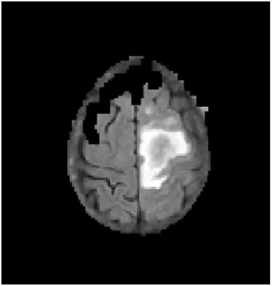
Pre-processing is the initial step in which images perform certain operations before segmentation. It is very essential because images in the database are the raw images and need to convert those images into some usable form before processing. Some of the pre-processing steps are used here such as Binarization, Enhancement and morphological operations. Binarization coverts input image into binary format as 0(black pixel value) and 1(white pixel value). It is done according to the threshold which is based on minimum variance in the class. The pixel values are processed to achieve desired enhancement. Binary images are distorted due to noise, so removal of noise is important to get higher accuracy of the system. Here noise reduction is done by morphological operation [13]. Original MR input image is shown in Fig 2 and pre-processed MR image is shown in Fig. 3.

C.Segmentation

The required Region of Interest (ROI) Extraction is done from the locale of the MR images. In this study, the aim of segmentation before classification is to detect the tumor region. Fuzzy c-mean and Skull Stripping [20], [22] is applied here for segmentation of MR images. Skull stripping is an essential step which segregates non-brain tissues like skull, scalp, fat, eyes etc. from anatomical images to enhance the speed and accuracy of diagnosis. Skull stripping is done after pre-processing of the MR images as shown in Fig. 4. Fuzzy C-Mean (FCM) is a

clustering technique for classifying the patterns that permits one place of data point connects to the two or more clusters [8], [11], [15]. Different data points belong to different type of cluster. Here data is bound to each cluster by mean of the membership function which indicates that the degree of data points belongs to appropriate cluster as presented in Fig. 5. FCM has been executed in this paper to increase the accuracy of different classification techniques [10].

D.Feature Extraction

It is performed by using Discrete Wavelet Transform (DWT) separating the important features from the segmented area of MR image. Haar Wavelet is a part of DWT which provides good result in respect of the extraction of the features and wavelet coefficients from MR images [18], [4]. DWT includes dynamic scales and positions, also use single prototype mother wavelet which is rescaled by powers of two and translated by integers. DWT gives adequate statistics both for synthesis and analysis of the original signal. DWT decomposes images into scaling functions and wavelet functions. Additional property of DWT is to remove Gaussian noise from the respective MR image.

Here High pass filters and Low pass filters are used. An image is decomposed into four sub bands indicated as LH (Low High filter), LL (Low Low filter), HH (High High filter) and HL (High Low filter), at level1 in the DWT domain. LL represents coarse-level coefficients where HL, LH and HH constitute the finest scale wavelet coefficients. Low frequency keeps more information, since human visual system is much more sensitive to the low-frequency part i.e. LL sub band. So here we use LL filter with one scale to enhance the quality of MR images. It decomposes the signal into one level using filtering decimation to obtain the approximation and detailed coefficient.

International Journal of Innovative Technology and Exploring Engineering (IJITEE) ISSN: 2278-3075,Volume-8 Issue-10, August 2019

Fig. 2 Input MR Image

Fig. 3 Pre-processed MR Image

Fig. 4 Skull Stripping of MR Image

Fig. 5 Image Segmentation

Table- I: Features are extracted from DWT method

S.No Features Value

1 Mean 22.82

2 Variance 5392.4

3 Max. Amplitude 510.0

4 Max. Energy 2.66

5 Min. Energy 0.11

6 Mean Frequency 4177.9

7 Max. Frequency 51745.0

8 Min. Frequency 266.08

9 Min. Amplitude 0.001

10 Mean Energy 5911.8

11 Mid Frequency 1620.8

12 Half Point Function 0.52187

The frequency vector is extracted from LL sub band using twelve features in Matlab environment. The features are Mean, Variance, Maximum Amplitude, Maximum Energy, Minimum Energy, Mean Frequency, Maximum Frequency, Minimum Frequency, Minimum Amplitude, Mean of Energy, Mid frequency, and half point of the function. The value of features extracted from DWT is shown in Table I.

E.Feature Reduction

Brain Tumor

enhance the soft tissues contrast. Without any prior knowledge, this technique is used to separate unknown signal source into statistically independent components, for example let us consider the party problem, when multiple people speak, so there is mixed signal, and ICA separates these signal sources. ICA seems a very effective technique to maximize the independency in image processing. For this, minimize the mutual information or maximize the non-Gaussianity. The values of reduced features extracted after DWT process are shown in Fig. 6.

Fig. 6 Features Extracted from DWT F. Classification

In this paper, we have compared three supervised classification technique that analyze the MR image to get better accuracy for the detection of brain tumor. Classification techniques [21] are Random Forest (RF), Artificial Neural Network (ANN) and Support Vector Machine (SVM). Here we compare different types of classifiers whose training and testing are executed to diagnosis the benign and malignant MR images. Three different types of classifiers used are discussed below:

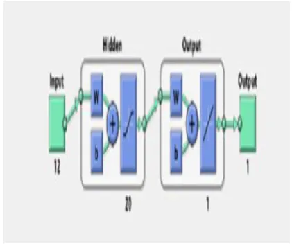
Random Forest (RF): RF is one of the most flexible and effective supervised machine learning algorithm classifiers that show the awareness of multiple peoples in different sectors [26]. It can be used for both classification and regression tasks. Here the approach used is to select the best feature from the random selection of features to get relevant and stable model. This split is taken randomly from a subset of optimum splits. Also, take more number of trees, randomly by adding random threshold for each feature. It calculates the comparative significance of each feature. Here RF shows maximum output in terms of Accuracy and AUC-ROC curve. Artificial Neural Network (ANN): It is a model which is based on the functions and structure of neural network named as neurons. It is a machine learning technique that works like the processing of human neurons [18], [24]. Neural Network structure looks like a graph which contains nodes as neurons which is connected, by arc as weights. It contains minimum three layers; first is the input layer, second is the hidden layer and last is the output layer. Also, activation function is used to sense something very complicated and complex functional mapping. Here twenty layers are used as hidden layer. The

diagram of ANN [27] which is implemented by Matlab is shown in Fig. 7. The outcome after the implementation of ANN classifier is shown in terms of accuracy, ROC-AUC, sensitivity, specificity and MCC. Support Vector Machine (SVM): A set of mathematical functions which is labeled as kernel. The main purpose of the kernel is to grab the data as input MR image and convert it into the required structure. Different types of kernel functions are used in different SVM algorithms. Here we focus on linear kernel [9], [13], [23]. The result after the execution of SVM classifier is shown in terms of accuracy, ROC-AUC, sensitivity, specificity and MCC in the experimental result.

Fig. 7 Diagram of ANN

III. EXPERIMENTALRESULT

Automatic detection of brain tumor through different stages of proposed methodology like segmentation, extraction of features and different classification has been done. A wide variety of database has been used. The proposed system is implemented on the given dataset of MR images and after execution of all the steps, in our computerized system, the result has been categorized according to the following evaluation parameters like AUC-ROC curve, Specificity, Sensitivity, Matthews’s coefficient correlation and Accuracy as shown in Table II. Sensitivity is true positive rate (TPR) or probability of detection of abnormalities which tells the proportion of actual positives that are correctly identified. Specificity is true negative rate (TNR) that is the actual negatives that represents the proportion of actual negative that are correctly identified [4]. Accuracy (ACC) represents proportion of both true positives and true negatives. Here TP is true positive that identify the positive cases (means abnormal brain identify as abnormal), TN is true negative that identify only negative cases (means normal brain identify as normal), FN is false negative that means abnormality is incorrectly identified as normal brain (False identification) and FP is false positive that means normal brain is wrongly identified as abnormal brain (False identification).True Positive Rate (TPR) = Number of True Positives (TP) / Total number of abnormalities in a given dataset (P). True Negative Rate (TNR) = Number of True Negatives (TN) /Total number of normality’s in a given dataset

International Journal of Innovative Technology and Exploring Engineering (IJITEE) ISSN: 2278-3075,Volume-8 Issue-10, August 2019

False Positive Rate (FPR) = Number of False Negatives (FP)/ Total number of normality’s in a given dataset (N).

ACC = (TP + TN / P + N)

Where P is TP [(True Positive) + FN (False Negative)] and N is TN [ (True Negative) + FP (False Positive)].

Matthews’s coefficient correlation (MCC) enables one to determine that how well the classification model is performing. It is a coefficient correlation between target and prediction which varies from -1 to 1. The values of MCC of SVM, RF and ANN are 0.9838, 0.9916 and 0.9705 respectively. Here 1 indicates completely correct agreement between actual and prediction, -1 indicates completely wrong disagreement between actual and prediction and 0 when the prediction may be random with respect to the actual. The MCC can be calculated using the confusion matrix using the formula [28]:

MCC= [(TP*TN-FP*FN)] [(TP+FP) (TP+FN) (TN+FP) (TN+FN)]

After calculating all the values of MCC with respect to all three classifiers, the result of RF is outstanding related to others.

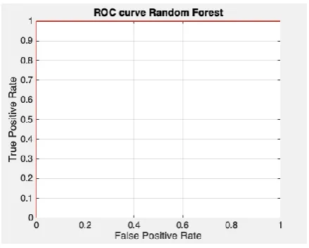
Area under the Curve-Receiver Operating Characteristic (AUC-ROC) is a graph which displays the implementation of a multi-class model many times with different classification thresholds settings having two parameters first is TPR and second is FPR [29]. ROC is a probability curve and AUC represents degree of separability. Model is better when AUC is higher which distinguishing the patient with disease and no disease. AUC-ROC curve for ANN, SVM and RF are plotted with TPR against the FPR as shown in Fig. 11, Fig. 12 and Fig. 13 respectively. In case of RF, AUC is 1 which means that it is perfectly able to distinguish between abnormality cases and normality cases. In SVM and ANN, AUC is 0.96 and 0.92 respectively which means that only 96% and 92% probability that the model will be able to differentiate between positive cases and negative cases.

Table- II: Different Evaluation Parameters for Different Classification Method

Tech. ACC TPR TNR MCC AUC-ROC

SVM 95.8333 0.9 1 0.983 0.96667

RF 100 1 1 0.991 1

ANN 91.6667 0.818 1 0.970 0.92308

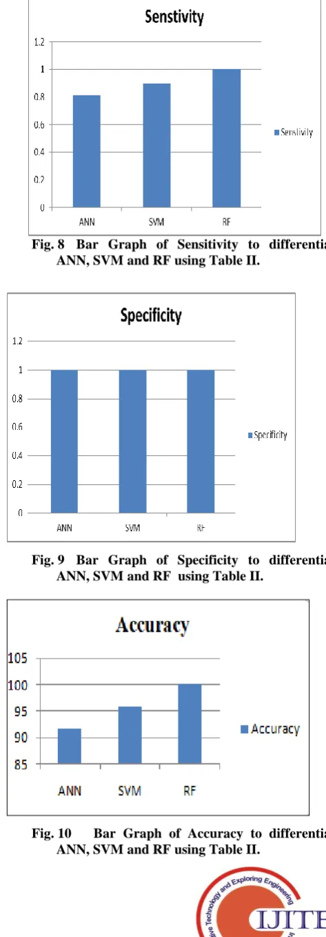
After simulation of our proposed work, we get to know about the exact value of evaluation of different classifiers. Here we have used 96 training datasets for SVM, RF and ANN classifiers respectively. After training the classifiers we undergo for testing the 24 MR images. Fig. 8, Fig. 9 and Fig. 10 respectively shows the bar graph of ANN, SVM and RF in terms of sensitivity, specificity and accuracy based on Table I. Our computerized system attains an accuracy rate at 95.83% for SVM, accuracy rate at 100% for RF, and accuracy rate at 91.6667% for ANN. We have also calculated the MCC and AUC-ROC of SVM, RF and ANN, their values are shown in Table II. After comparing all the classification techniques, it

is observed that the accuracy rate and AUC-ROC curve of RF are higher than SVM than ANN. After the diagnosis of the tumor by this computerized system, the final decision would be suggested by radiologist.

Fig. 8 Bar Graph of Sensitivity to differentiate ANN, SVM and RF using Table II.

Fig. 9 Bar Graph of Specificity to differentiate ANN, SVM and RF using Table II.

Brain Tumor

Fig. 11 AUC-ROC Curve for ANN

Fig. 12 AUC-ROC Curve for SVM.

Fig. 13 AUC-ROC Curve for RF.

IV. CONCLUSIONANDFUTUREWORK

Medical image processing is an important tool for knowledge discovery from medical data and is widely used to detect the abnormalities in the brain or other parts of the body through different modalities. It has become one of the major research subjects in medical field. In this paper we have executed

different types of machine leaning techniques applied to MRI modality. Different statistical parameters have been taken for the assessment of different classification techniques. The experimental results have shown that Random Forest classifier achieves the highest accuracy rate than the other two. Also, real MRI dataset has been used to get more precise outcomes.

Detection of brain tumor is still an open research problem. The system can be made more stable by using more number of dataset. The proposed methodology could be more useful for the detection of different types of abnormalities. In order to improve the accuracy of final outcome, new algorithm may be proposed at the initial stage i.e. ROI extraction because extracting the region of tumor is important and should be properly identified. Also, an intelligent and hybrid method could be proposed for machine learning in order to enhance the quality of the computerized system by extracting more appropriate features. Obtaining high quality MR image itself is another challenging issue and can be further explored. Neural Network performance may be improved by increasing numbers of layers.

ACKNOWLEDGMENT

This research work has been possible by implementing the real MRI images provided by Maharaja Agrasen Hospital, Punjabi Bagh, New Delhi. Hence we would like to extend our sincere gratitude to the management as well as neurological Department of the Hospital for providing required amount of logistical support.

REFERENCES

1. American Society of Clinical Oncology (ASCO), http://www.asco.org/.

2. Gonzalez, R. C., & Woods, R. E. (2008). Digital image processing (3rd

ed.). Pearson Prentice Hall (Prentice Hall, 2002).

3. E.-S. A. El-Dahshan, H. M. Mohsen, K. Revett, & A.-B. M. Salem, “Computer-aided diagnosis of human brain tumor through MRI: A survey and a new algorithm”, Expert Systems with Applications, vol. 41, pp. 5526–5545, 2014.

4. F. P. Polly, S. K. Shil, M. A. Hossain, A. Ayman, & Y. M. Jang, “Detection and Classification of HGG and LGG Brain Tumor Using Machine Learning”, International Conference on Information Networking (ICOIN), pp. 813-817, 2018.

5. E. Dandil, M. Cakiroglu, Z. Eksi, “Computer-aided diagnosis of malign

and benign brain tumors on MR images”, International Conference on ICT Innovations, pp. 157–166, 2014.

6. Midas: healthy human brain database. Available online:

http://www.insightjournal.org/midas/collection/view/27

7. Brainweb (2014). Brainweb: Simulated brain

database.<http://brainweb.bic.mni.mcgill.ca/cgi/brainweb2>

8. M. A. Balafar, “Fuzzy C-mean based brain MRI segmentation

algorithms”, Artificial Intelligence Review, vol. 41, pp. 441- 449, 2014. 9. Gasmi, K., Kharrat, A., Messaoud, M. B., & Abid, M., “Automated segmentation of brain tumor using optimal texture features and support vector machine classifier”, International Conference on Image Analysis and Recognition LNCS, pp. 230–239, 2012.

10. Jafari, M., & Kasaei, S., “Automatic brain tissue detection in MRI images using seeded region growing segmentation and neural network classification”, Australian Journal of Basic and Applied Sciences, vol. 5(8), pp.1066–1079, 2011.

International Journal of Innovative Technology and Exploring Engineering (IJITEE) ISSN: 2278-3075,Volume-8 Issue-10, August 2019

12. Tabatabai, G., Stupp, R., Bent, M. J., Hegi, M.E., Tonn, J.C., Wick, W.,

& Weller, M., “Molecular diagnostics of gliomas: the clinical perspective”, Acta Neuropathologica, vol. 120, pp. 585– 592, 2010. 13. Chaplot, S., Patnaik, L.M., & Jagannathan, N.R., “Classification of

magnetic resonance brain images using wavelets as input to support vector machine and neural network”, Biomedical Signal Processing and Control, vol. 1, pp. 86-92, 2006.

14. Van Meir, E.G., Hadjipanayis, C.G., Norden, A.D., Shu, H.K., Wen, P.Y., & Olson, J.J., “Exciting new advances in neuro- oncology: theavenue to a cure for malignant glioma”, A Cancer Journal for Clinicians, vol. 60, pp. 166–193, 2010.

15. Phillips, R. Velthuizen,S. Phupanich, L. Hall, L. Clarke, & M. Silbiger, “Application of fuzzy C-means segmentation technique for tissue differentiation in MR images of a hemorrhagic glioblastoma multiform”, Magnetic Resonance Imaging, vol. 29, pp. 277–290, 1995.

16. Khotanlou, H., Colliot, O., Atif, J., & Bloch, I., “3D brain tumor segmentation in MRI using fuzzy classification, symmetry analysis and spatially constrained deformable models”, Fuzzy Sets and System, vol. 160, pp. 1457-1473, 2009.

17. A. E. Lashkari, “A Neural Network based Method for Brain Abnormality

Detection in MR Images Using Gabor Wavelets”, International Journal of Computer Applications, vol. 4, pp.841- 1140, 2010.

18. Pauline, J., “Brain Tumor Classification Using Wavelet and Texture Based Neural Network”, International Journal of Scientific & Engineering Research, vol. 3, pp.1–7, 2012.

19. Kolen, J.F., Hutcheson, T., “Reducing the time complexity of the fuzzy

c-means algorithm”, IEEE Transactions on Fuzzy Systems, vol. 10, pp.263–267, 2002.

20. Murugavalli, S., Rajamani, V., “A high speed parallel fuzzy c- mean algorithm for brain tumor segmentation”, Bioinform. Medical Engineering Journal, vol. 6, pp.29–34, 2006.

21. Zacharaki, E.I., Wang, S., Chawla, S., Yoo, D.D., Wolf, R., Melhem, E.R., & Davatzikos, C., “Classification of Brain Tumor Type and Grade Using MRI Texture and Shape in a Machine Learning Scheme”, Magnetic Resonance in Medicine, vol. 62, pp. 1609–1618, 2009. 22. Gambino, O., Daidone, E., Sciortino, M., Pirrone, R., & Ardizzone, E.,

“Automatic Skull Stripping in MRI based on Morphological Filters and Fuzzy C-means Segmentation”, Annual International Conference of the IEEE Engineering in Medicine and Biology Society, pp.5040-5043, 2011.

23. Bahadure, N.B., Ray, A.K., & Thethi, H.P., “Image Analysis for MRI

Based Brain Tumor Detection and Feature Extraction Using Biologically Inspired BWT and SVM”, Hindawi International Journal of Biomedical Imaging, vol. 2017, pp. 1- 12, 2017.

24. AyseDemirhan, Mustafa Toru, InanGuler, “Segmentation of Tumor and

Edema Along with healthy tissues of brain using Wavelets and Neural Networks”, IEEE Journal of Biomedical and Health Informatics, vol.19, pp.1451-1458, 2015.

25. Dipali M Joshi, Rana N K & Misra VM, “Classification of Brain Cancer

Using Artificial Neural Network”, IEEE Conference on Electronic Computer Technology(ICECT), pp.112-116, 2010.

26. L. Breiman, Random forests, Machine learning, vol. 45, pp. 5- 32, 2001.

27. S. Haykin, Neural Networks: A Comprehensive Foundation, second ed.,

PHI, 1994.

28. D. M. W. Powers, Evaluation: From Precision, Recall and F- Measure to

ROC, Informedness, Markedness & Correlation, 2011, vol. 2, pp. 37-63. 29. T. Fawcett. (2006, June). An Introduction to ROC Analysis. Pattern

Recognition Letters. vol. 27, pp. 861-874.

AUTHORSPROFILE

Manu Singh received her BTech in Computer

Science & Engg. from SCRIET, Meerut (UP) in 2007, Mtech from Shobhit University, Meerut (UP) in 2011 and doing PhD from Guru Gobind Singh Indraprastha University, Delhi. Her area of interest is Computer Science & Engineering, Image Processing and Networking. She has published six papers in different journals.

Dr. Vibhakar Shrimali received his BE

(Electronics & Communication Engineering) in 1988 from MBM Engineering College Jodhpur (Raj), ME (Electronics & Communication Engg.) in 2003 from Delhi College of Engg. (Delhi) and PhD from IIT Roorkee in 2009. His field of interest