Explicit fiber beam-column elements for impact analysis of structures

City, University of London Institutional Repository

Citation

:

This is the accepted version of the paper.

This version of the publication may differ from the final published

version.

Permanent repository link: http://openaccess.city.ac.uk/19284/

Link to published version

:

Copyright and reuse:

City Research Online aims to make research

outputs of City, University of London available to a wider audience.

Copyright and Moral Rights remain with the author(s) and/or copyright

holders. URLs from City Research Online may be freely distributed and

linked to.

City Research Online: http://openaccess.city.ac.uk/ publications@city.ac.uk

1

EXPLICIT FIBER BEAM-COLUMN ELEMENTS FOR IMPACT ANALYSIS OF

STRUCTURES

Samer Sabry F. Mehanny Gendy (1), Ashraf Ayoub (2)

1

Ph.D. Candidate, School of Mathematics, Computer Science & Engineering, Department of Civil Engineering; City, University of London, London, UK; E-mail: Samer.Gendy@city.ac.uk

2

(corresponding author) Professor, School of Mathematics, Computer Science & Engineering, Department of Civil Engineering; City, University of London, London, UK; E-mail: Ashraf.Ayoub.1@city.ac.uk

Abstract

The solution of impact problems requires advanced computational techniques to overcome

the difficulties associated with large short-duration loads. In this case, the explicit time

integration method is typically used, since it provides a stable solution for problems such as

the analysis of structures subjected to shock and impact loads. However, most explicit-based

finite elements were developed for continuum models such as membrane and solid elements,

which renders the problem computationally expensive. On the other hand, the development of

fiber-based beam finite elements allows for the simulation of the global structural behavior

with very few degrees of freedoms, while accounting for the detailed material nonlinearity

along the element length. However, explicit-based fiber beam elements have not been

properly formulated, in particular for the case of the emerging force-based beam element.

In this paper, two developed fiber plane beam elements that consider an explicit time

integration scheme for the solution of the dynamic equation of motion are presented. The first

element uses a displacement-based formulation, while the second element uses a force-based

formulation. For the latter case, a new algorithm that eliminates the need for iterations at the

element level is proposed. The developed elements require the use of a lumped mass matrix

2

are required, which renders the problem numerically efficient. The developed explicit fiber

beam-column models, particularly the force-based element, represents a simple yet powerful

tool for simulating the nonlinear complex effect of impact loads on structures accurately

while using very few finite elements. The traditional implicit method of analysis typically

fails to provide numerical stable behavior for such short time duration problems.

Two correlation studies are presented to highlight the efficiency of the developed elements in

modelling impact problems where the strain rate effect is considered in the material models.

These examples confirm the accuracy and efficiency of the presented elements.

KEY WORDS

Explicit analysis, fiber beam modelling, drop weight impact test, force-based element,

displacement-based element.

INTRODUCTION

The fiber beam element is known to be an advanced and numerically efficient element for the

analysis of nonlinear dynamic problems (Spacone et al. 1996, Neuenhofer and Filippou

1997, Mullapudi and Ayoub 2010). However, the existing fiber beam elements use an

implicit time integration method that requires a large number of iterations per time step to

reach convergence. In several dynamic analyses, particularly for impact and blast problems,

the solution cannot be achieved due to severe numerical difficulties (Bathe and Cimento

3

Meanwhile, commercial finite element software programs are widely used to model impact

problems using the explicit algorithm. However, most of the elements used for these types of

analysis are continuum-based elements. Huang and Wu (2009) studied the dynamic impact

of a vertical concrete cask tip-over using the explicit capability in the software LS-DYNA.

Hong et al. (2014) created a numerical model to simulate the response of non-composite

steel-concrete-steel sandwich panels under impact loading using the same software. Recently,

Chen et al. (2016) simulated the effect of a large-size truck hitting a reinforced concrete

column using also LS-DYNA. In all these studies, solid elements were used to simulate the

impact problems. These models required considerable execution time, large storage memory,

and slow post-processing. On the other hand, the fiber plane beam element requires much less

storage size, smaller execution time, and fast post-processing.

Moreover, several researchers used the explicit time integration technique to solve different

structural problems under dynamic loading. Kujawski (1988) presented a semi-explicit

algorithms for dynamic non-linear problems using iteratively only forward substitution that

allows the utilization of both consistent and lumped mass matrix. Miranda et al. (1989)

derived an explicit predictor-corrector algorithm from the implicit alpha-method. It was

found that the explicit algorithm has a better stability and higher accuracy when compared

with a Newmark-based predecessor. The algorithm is utilized for the solution of linear and

non-linear structural dynamics problems. Pezeshk and Camp (1995) developed an explicit

time integration technique for dynamic analyses of linear undamped single degree of freedom

systems. The technique was based on a modified trapezoidal rule to approximate the

governing ordinary differential equation. It was found that the new explicit procedure is more

accurate in determining the transient response with the same amount of computational cost

4

Sun et al. (2000) compared the performance of an implicit and explicit finite element

methods for two dynamic problems (an elastic bar and a cylindrical disk on a rigid wall)

using the ABAQUS finite element software. For the fast linear contact problems, it was found

that the advantages of the explicit method are apparent within a desirable tolerance.

Chang (2009) presented a new explicit method with enhanced stability. The new explicit

method have unconditional stability for general instantaneous stiffness hardening systems in

addition to linear elastic and instantaneous stiffness softening systems, where the

instantaneous stiffness is a parameter used by the author to describe the variation of stiffness

for a non-linear system. It was found that the new method is efficient for the solution of a

general structural dynamic problems where the response is dominated by low-frequency

modes and when high frequency responses are of no interest. The method was also found to

be second-order accurate.

Fulei and Yungui (2011) used the finite rotation theory to determine the node direction

vectors and the Yoshida method (Yoshida et al. 1980) to find the element direction vectors

of a nonlinear beam element. The authors formulated their element in a corotational system

and used an explicit algorithm for the solution of nonlinear dynamic structures. The authors

compared their results with the ANSYS explicit commercial software.

Lately, Tenek (2015) presented a three-dimensional explicit beam finite element with the

derivation of an initial load due to temperature. The element was employed to analyse beams,

arches, and frame structures.

Many of the previously published work concentrated on employing simple material models.

However, the accurate prediction of the complex structural response requires more rigorous

material models able to depict the performance of the structure under severe loading

5

elements use advanced nonlinear material models for both concrete and steel members for the

accurate representation of nonlinear behaviour along the element length. The developed

elements are implemented in the research-oriented finite element analysis program FEAP

developed by Taylor (2014).

EXPLICIT AND IMPLICIT TIME INTEGRATION METHODS

Explicit dynamic analysis is a mathematical method for integrating the equations of motion

through time. The explicit procedure is suitable for high-speed short time duration analysis as

stated by Gu and Wu (2013). It is conditionally stable, which means that a small time

increment has to be used to ensure that the solution is stable. So, longer analysis runtime

should be expected in the explicit analysis.

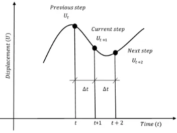
In the explicit analysis, dynamic values for the current step are obtained from values already

known from the previous step by solving for time (𝑡 + ∆𝑡) using values from the preceding

time(𝑡), where (𝑡) is the time elapsed and (∆𝑡) is the time increment as shown in Fig. (1). Also no convergence check is needed as the nodal accelerations are calculated directly by

multiplying the inverse of the mass matrix by the force vector.

However, in the implicit method, values for the next step are obtained from values from both

the current step and the later one by solving for time (𝑡 + ∆𝑡) using data from time (𝑡) and

(𝑡 + ∆𝑡). Thus a Newton-Raphson iteration technique is essential to find the solution and to

enforce equilibrium by iterating until convergence is achieved.

Therefore, the explicit method is conditionally stable with no required convergence checks,

necessitates many relatively inexpensive time steps, and is suitable for short transient

6

entails convergence checks at all times, requires small number of expensive time steps, and is

typically suitable for static and quasi static problems. In general, the implicit method can lead

to convergence problems as it is more sensitive to initial conditions and non-linear behavior.

STABILITY OF THE EXPLICIT METHOD

The explicit method gives accurate solution as long as the numerical stability is maintained,

which is known as a conditionally stable method. Therefore a small time step is required for

explicit analysis and the time step should be assessed before attempting the solution. In this

process, the chosen time increment (∆𝑡) must be less than the stable time increment(∆𝑡_𝑚𝑖𝑛).

The stable time increment is calculated by:

Δt_𝑚𝑖𝑛 =_𝑐𝐿

𝑑 (1)

where 𝑐_𝑑 is the dilatational wave speed, 𝑐_𝑑 = √𝐸_𝜌 (2)

𝐸 is the material Young’s modulus, 𝜌 is the material density and 𝐿 is the element length.

Decreasing 𝐿 or increasing 𝑐_𝑑 will reduce the stable time increment.

DYNAMIC FORMULATION OF THE EXPLICIT METHOD

The dynamic equilibrium equation of motion that describes the motion of a body subjected to

a force can be generally written in the following form:

𝑀𝑈̈_𝑡+ 𝐶𝑈̇_𝑡+ 𝐾𝑈_𝑡= 𝐹_𝑡 (3)

Where 𝑀 is the mass matrix and 𝐾 is the stiffness matrix, 𝐹𝑡 is the vector of external forces

and 𝑀𝑈̈_𝑡 represents the inertia force while 𝐶𝑈̇_𝑡 represents the damping force.

7

𝐶 = 𝛼𝑚𝑀 + 𝛽𝑘𝐾 (4)

Where 𝛼𝑚 is the mass proportional Rayleigh damping parameter and 𝛽𝑘 is the stiffness

proportional Rayleigh damping parameter. They are calculated based on the natural

frequencies of the first modes and their damping ratios. The solution of the dynamic equation

of motion for the developed beam elements is conducted in the corotational reference frame

as described next.

COROTATIONAL FORMULATION OF THE DEVELOPED FIBER BEAM

ELEMENTS

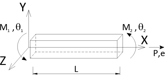
The presented elements are formulated in the corotational frame where the rigid body modes

are removed before the dynamic effect is added in the global frame. The corotational element

has three natural degrees of freedom, an axial elongation 𝑒 and two rotations 𝜃₁ and 𝜃₂ at each end of the element. The axial force 𝑃 and the moments 𝑀₁ and 𝑀₂ at both ends are the corresponding element nodal forces and are shown in Fig. (2). The global frame consists of

six degrees of freedom (four translations and two rotations) and six corresponding forces.

Next, the explicit formulations used in this paper are discussed in details.

EXPLICIT FORMULATION OF THE DISPLACEMENT-BASED ELEMENT

In the first explicit fiber beam element a displacement-based formulation is used where

equilibrium is satisfied in a weighted integral sense.

The internal and external forces, (𝐹_{𝑖𝑛𝑡𝑒𝑟𝑛𝑎𝑙} and 𝐹_{𝑒𝑥𝑡𝑒𝑟𝑛𝑎𝑙}) respectively, are summed at each node point, and the nodal accelerations are computed by multiplying the forces with the

inverse of the nodal mass:

8

The explicit algorithm uses the Newmark beta-gamma method with the primary variables

being displacement increments to calculate the displacement, velocity and acceleration.

Accordingly, the solution to Equation (3) leads to the following:

𝑈_𝑡+1 = 𝑈_𝑡+ ∆𝑡𝑈̇_𝑡+1₂(1 − 𝛽)∆𝑡2_𝑈̈

𝑡+1₂𝛽∆𝑡2𝑈̈𝑡+1 (6)

𝑈̇_𝑡+1= 𝑈̇_𝑡+ (1 − 𝛾)∆𝑡𝑈̈_𝑡+ 𝛾∆𝑡𝑈̈_𝑡+1 (7)

𝑀𝑈̈𝑡+1+ 𝐶𝑈̇𝑡+1+ 𝐾𝑈𝑡+1− 𝐹𝑡+1= 0 (8)

For an implicit solution, 𝛽 = 0.25 and 𝛾 = 0.5, while the explicit algorithm assume

𝛽 = 0 and 𝛾 = 0.5, then calculate the acceleration 𝑈̈_𝑡 at time (t) by making use of the

inversion of the mass matrix based on equation (5), followed by calculating the displacement

𝑈𝑡+1 using equation (6). The evaluation of the mass matrix is described in detail in a

subsequent section. The velocity𝑈̇_𝑡+1and the acceleration 𝑈̈_𝑡+1 are then calculated explicitly at time (t+1) by using the two equations (7) and (8).

The algorithm starts by assuming an Explicit Parameter to equal 1 for explicit dynamic

analysis.

The equivalent global dynamic stiffness 𝐾̂_{𝑒𝑙𝑒𝑚(𝑔𝑙𝑜𝑏𝑎𝑙)}is substituted by the lumped mass matrix:

𝐾̂_{𝑒𝑙𝑒𝑚(𝑔𝑙𝑜𝑏𝑎𝑙)}𝑡+1 _{= 𝐸𝑥𝑝𝑙𝑖𝑐𝑖𝑡 𝑃𝑎𝑟𝑎𝑚𝑒𝑡𝑒𝑟 × 𝑀 (9)}

And the global internal dynamic load 𝐹̂_{𝑒𝑙𝑒𝑚(𝑔𝑙𝑜𝑏𝑎𝑙)} is determined as:

𝐹̂_{𝑒𝑙𝑒𝑚(𝑔𝑙𝑜𝑏𝑎𝑙)}𝑡+1 = 𝐹_{𝑒𝑙𝑒𝑚(𝑔𝑙𝑜𝑏𝑎𝑙)}𝑡+1 + 𝑀 𝑈̈𝑡+1_{+ (𝛼}

𝑚𝑀 + 𝛽𝑘𝐾)𝑈̇𝑡+1 (10)

9

into fibers with prescribed nonlinear material behaviour. The global element force increment

is:

Δ𝐹̂_{𝑒𝑙𝑒𝑚(𝑔𝑙𝑜𝑏𝑎𝑙)}𝑡+1 = 𝐹̂_{𝑒𝑥𝑡𝑒𝑟𝑛𝑎𝑙}𝑡+1 − 𝐹̂_{𝑒𝑙𝑒𝑚(𝑔𝑙𝑜𝑏𝑎𝑙)}𝑡+1 (11)

Where 𝐹̂_{𝑒𝑥𝑡𝑒𝑟𝑛𝑎𝑙} is the applied external force corresponding to the load step.

Then at the global level, the finite element solution for an acceleration increment in the global

frame ∆𝑈̈(𝑔𝑙𝑜𝑏𝑎𝑙) is computed by:

Δ𝑈̈_{(𝑔𝑙𝑜𝑏𝑎𝑙)}𝑡+1 = [𝑘̂_{𝑒𝑙𝑒𝑚(𝑔𝑙𝑜𝑏𝑎𝑙)}𝑡+1 ]−1× Δ𝐹̂_{𝑒𝑙𝑒𝑚(𝑔𝑙𝑜𝑏𝑎𝑙)}𝑡+1 (12)

In the explicit solution, Δ𝑈 is then calculated from ∆𝑈̈(𝑔𝑙𝑜𝑏𝑎𝑙) using equations (6 to 8) as

detailed before.

The evaluation of the stiffness matrix 𝐾𝑒𝑙𝑒𝑚 and load vector 𝐹𝑒𝑙𝑒𝑚 is first calculated in the

corotational frame, then transformed to the global frame by adding the rigid body modes as

follows:

𝑘_{𝑒𝑙𝑒𝑚(𝑔𝑙𝑜𝑏𝑎𝑙)}𝑡+1 = 𝑇𝑇 _𝐾

𝑒𝑙𝑒𝑚𝑡+1 𝑇 (13)

𝐹_{𝑒𝑙𝑒𝑚(𝑔𝑙𝑜𝑏𝑎𝑙)}𝑡+1 _{= 𝑇}𝑇 _𝐹

𝑒𝑙𝑒𝑚𝑡+1 (14)

Where 𝑇 is the transformation matrix = [

−1 0 0 1 0 0

0 1_𝐿 1 0 −1_𝐿 0 0 1_𝐿 0 0 −1_𝐿 1

] (15)

To determine the value of 𝐾_{𝑒𝑙𝑒𝑚} and 𝐹_{𝑒𝑙𝑒𝑚} using the displacement-based method in the corotational frame, the section deformation increment of the element reference axis in the

corotational frame is first evaluated as:

10

Where 𝑆 is the displacement shape function = [

1

𝐿 0 0

0 −4_𝐿 +6 𝑥_𝐿 −2_𝐿 +6 𝑥_𝐿 ] (17)

The calculation of the displacement increment ∆𝑞 in the corotational frame is accomplished

using the matrix 𝑇:

∆𝑞𝑡+1_{= 𝑇 ∆𝑈}𝑡+1 ₍₁₈₎

The element stiffness can then be calculated as:

𝐾_{𝑒𝑙𝑒𝑚}𝑡+1 _{= ∫ 𝑆}𝑇 _𝑘

𝑠𝑒𝑐𝑡+1 𝑆 𝑑𝑥 𝐿

0 (19)

Where 𝑘𝑠𝑒𝑐 is the section stiffness. And the element internal resisting force vector is equal to:

𝐹_{𝑒𝑙𝑒𝑚}𝑡+1 = ∫ 𝑆𝑇 _𝐹

𝑠𝑒𝑐𝑡+1 𝑑𝑥 𝐿

0 (20)

Where 𝐹_𝑠𝑒𝑐 is the section resisting forces in the corotational frame.

𝐹_𝑠𝑒𝑐𝑡+1_{= {}𝑝

𝑀} (21)

Where 𝑝 is the section axial force and 𝑀 is the section bending moment.

The section stiffness 𝑘_𝑠𝑒𝑐 and force vector 𝐹_𝑠𝑒𝑐 are determined from fiber discretization as noted earlier using the section deformation increment and following the assumption of plane

sections remaining planes:

𝜀1 (𝑥, 𝑦) = 𝜀(𝑥) − 𝑦 ∅(𝑥) (22)

Where 𝜀1 is the fiber axial strain, 𝜀 is the axial strain at the beam axis, 𝑦 is the distance from

the neutral axis, and ∅ is the section curvature. The fiber strain is used along with the fiber nonlinear material constitutive law to determine the fiber force and stiffness, which are

11

The second order analysis is considered into the formulations by adding the geometric

stiffness matrix (Alemdar and white 2005).

Concisely to consider the second order effect, the stiffness matrix must be updated by adding

the internal geometric stiffness matrix term 𝐾_𝑔:

𝐾_{𝑒𝑙𝑒𝑚}𝑡+1 _{= (𝐾}

𝑔𝑡+1+ ∫ 𝑁₀𝐿 𝛿𝑇 𝑘𝑠𝑒𝑐𝑡+1 𝑁𝛿𝑑𝑥) (23)

Where 𝐾_𝑔𝑡+1= 𝑃𝑡+1[

2𝐿 15 −𝐿 30 0 −𝐿 30 2𝐿 15 0

0 0 0

] (24)

And 𝑃 is the axial force in the corotational frame.

Therefore equation (19) is replaced by equation (23) and the resisting load vector is evaluated

by:

𝐹_{𝑒𝑙𝑒𝑚}𝑡+1 = ∫ 𝑁₀𝐿 𝛿𝑇 𝐹𝑠𝑒𝑐𝑡+1 𝑑𝑥 (25)

Where 𝑁_𝛿 =

[

1

𝐿 (1 − 4𝑥 + 3𝑥2)2𝜃1+ (1 − 4𝑥 + 3𝑥2)(−2𝑥 + 3𝑥2)𝜃1+

(1 − 4𝑥 + 3𝑥2_{)(−2𝑥 + 3𝑥}2_)𝜃

2 (2𝑥 + 3𝑥2)2𝜃2

0 −4_𝐿+6𝑥_𝐿 −2_𝐿+6𝑥_{𝐿 ]}

(26)

So equation (20) is substituted by equation (25).

EXPLICIT FORMULATION OF THE FORCE-BASED ELEMENT

In the second explicit fiber beam element, a force-based formulation is used where the

equilibrium is satisfied in a section by section basis along the element length. In the newly

12

conducted once to calculate the element stiffness matrix and load vector. The use of this

technique is accurate as long as the time step is set to be smaller than a critical value.

However, if adopting a time step larger than the critical value, performing internal iterations

would be needed to minimize the internal residual error. In this case, the solution is

transformed into a mixed explicit implicit approach.

Equations (5 to 8) are used to calculate the global acceleration, velocity and displacement

explicitly at time (t+1). The dynamic stiffness 𝐾̂_{𝑒𝑙𝑒𝑚(𝑔𝑙𝑜𝑏𝑎𝑙)} and the dynamic load

𝐹̂_{𝑒𝑙𝑒𝑚(𝑔𝑙𝑜𝑏𝑎𝑙)}are then evaluated using equations (9 & 10).

Here 𝐾_{𝑒𝑙𝑒𝑚} and 𝐹_{𝑒𝑙𝑒𝑚} are determined using a force-based procedure in the corotational reference frame.

The same matrix T described in equation (15) is used to transform the system to a

corotational frame. ∆𝑞𝑡+1 is again evaluated using equation (18).

First the element initial end force increments are calculated with the use of the stiffness of the

element at the previous step:

Δ𝐹_{𝑒𝑙𝑒𝑚}𝑡+1 = 𝐾_{𝑒𝑙𝑒𝑚}𝑡 ∆𝑞𝑡+1 ₍₂₇₎

Then the new element end forces 𝐹_{𝑒𝑙𝑒𝑚}𝑡+1 are updated by Δ𝐹_{𝑒𝑙𝑒𝑚}𝑡+1 :

𝐹_{𝑒𝑙𝑒𝑚}𝑡+1 _{= 𝐹}

𝑒𝑙𝑒𝑚𝑡 + Δ𝐹𝑒𝑙𝑒𝑚𝑡+1 (28)

Where (𝑡 + 1) denotes the new increment step and (𝑡) denotes the previous step as the

external load is imposed in an incremental sequence.

Using the force interpolation function, the section force increments Δ𝐹𝑠𝑒𝑐 are determined by:

13

Where 𝑏 is the force interpolation function and can be expressed as = [1 0 0

0 1 − 𝑥 𝑥] (30)

The total section forces 𝐹_𝑠𝑒𝑐(𝑥)𝑡+1 are calculated by adding the section force increments

Δ𝐹_𝑠𝑒𝑐𝑡+1 _{to the previous section forces 𝐹}

𝑠𝑒𝑐𝑡 (𝑥):

𝐹_𝑠𝑒𝑐𝑡+1_{(𝑥) = 𝐹}

𝑠𝑒𝑐𝑡 (𝑥) + Δ𝐹𝑠𝑒𝑐𝑡+1 (31)

The section deformation increments are at that point established by the linearization of the

section force-deformation and then used to update the section deformation 𝑑_𝑠𝑒𝑐𝑡 .

𝑑_𝑠𝑒𝑐𝑡+1_{= 𝑑}

𝑠𝑒𝑐𝑡 + 𝑓𝑠𝑒𝑐𝑡+1 Δ𝐹𝑠𝑒𝑐𝑡+1 (32)

Where 𝑓𝑠𝑒𝑐𝑡+1 is the section flexibility calculated from the fibers.

To avoid violating the equilibrium, the section unbalanced forces are considered; which are

the difference between the calculated total section forces and the section resisting forces. The

section resisting forces are evaluated from discretization of the section into fibers using the

updated section deformation 𝑑_𝑠𝑒𝑐𝑡+1 and following the assumption of plane sections remaining planes:

𝐹𝑈𝑡+1(𝑥) = 𝐹𝑠𝑒𝑐𝑡+1(𝑥) − 𝐹𝑅𝑡+1(𝑥) (33)

Where FU is the section unbalance force vector, and FR is the resisting force vector. And

thereafter the unbalanced forces are converted to a residual section deformation r(x) using the

current section flexibility:

𝑟𝑡+1_{(𝑥) = 𝑓}

𝑠𝑒𝑐𝑡+1 𝐹𝑈𝑡+1(𝑥) (34)

The residual element deformations is then calculated by integrating the residual section

deformations along the element length:

𝑅𝑡+1_{= ∫ 𝑏}𝑙 𝑇_{(𝑥) 𝑟}𝑡+1_{(𝑥) 𝑑𝑥}

14

To insure numerical stability of the force based element, the residual R has to be minimized

to a very small acceptable value. In the implicit force-based algorithm, an element iteration is

needed in order to eliminate the section residual deformation 𝑟. This is performed using the

following energy criteria:

∑ 𝐹 31 𝑢𝑛𝑏𝑎𝑙𝑎𝑛𝑐𝑒𝑑∙Δq ≤ 𝑎𝑏𝑠𝑜𝑙𝑢𝑡𝑒 𝑡𝑜𝑙𝑒𝑟𝑎𝑛𝑐𝑒 (36)

Where 𝐹 𝑢𝑛𝑏𝑎𝑙𝑎𝑛𝑐𝑒𝑑 is the difference between the applied force and the resisting force.

In the explicit algorithm, a similar approach could be used, which requires an element-level

iteration until convergence is achieved. However, the element iteration becomes unnecessary

if the analysis time step is sufficiently small to satisfy the previous energy condition.

In this case, (∑ 𝐹 3_{1 𝑢𝑛𝑏𝑎𝑙𝑎𝑛𝑐𝑒𝑑}∙Δq) is compared to the ‘𝑎𝑏𝑠𝑜𝑙𝑢𝑡𝑒 𝑡𝑜𝑙𝑒𝑟𝑎𝑛𝑐𝑒’ for each element; and if found smaller this means that the element converges with one iteration only.

If found larger, however, the algorithm calculates a new critical time step Δt_{𝑐𝑟𝑖𝑡𝑖𝑐𝑎𝑙} :

Δt𝑐𝑟𝑖𝑡𝑖𝑐𝑎𝑙 𝑛𝑒𝑤 = Δt𝑐𝑟𝑖𝑡𝑖𝑐𝑎𝑙 𝑜𝑙𝑑 × √𝑎𝑏𝑠𝑜𝑙𝑢𝑡𝑒 𝑡𝑜𝑙𝑒𝑟𝑎𝑛𝑐𝑒 _{∑ 𝐹}

𝑢𝑛𝑏𝑎𝑙𝑎𝑛𝑐𝑒𝑑∙

3

1 Δq (37)

Where the tolerance value is typically varied between 10−4 to 10−8 depending on the problem being analysed and the accuracy desired by the user.

Finally, the chosen Δt_{𝑐𝑟𝑖𝑡𝑖𝑐𝑎𝑙} is the minimum Δt_{𝑐𝑟𝑖𝑡𝑖𝑐𝑎𝑙} of all elements. Hence, the time step is reduced to equal Δt_{𝑐𝑟𝑖𝑡𝑖𝑐𝑎𝑙} .

Therefore in addition to the condition of the stable time increment ∆𝑡_𝑚𝑖𝑛 , if the time step is smaller than or equal to Δt_{𝑐𝑟𝑖𝑡𝑖𝑐𝑎𝑙} , a single iteration is sufficient to satisfy the element-level convergence criteria described in (37), and the entire solution algorithm would not require

15

Once the element residual deformations are reduced to within the specified tolerance value,

the element end resisting forces are updated and the element flexibility 𝑓_{𝑒𝑙𝑒𝑚} is estimated by the integration of the section flexibility 𝑓_𝑠𝑒𝑐 along the element length. Then the element stiffness 𝐾_{𝑒𝑙𝑒𝑚} is computed by inverting the flexibility of the element.

(𝐾_{𝑒𝑙𝑒𝑚}𝑡+1 ₎−1 _{= 𝑓}

𝑒𝑙𝑒𝑚𝑡+1 = ∫ 𝑏₀𝐿 𝑇𝑓𝑠𝑒𝑐𝑡+1 𝑏 𝑑𝑥 (38)

And as a last step, the forces and deformations of all sections are updated using the new

element end resisting forces.

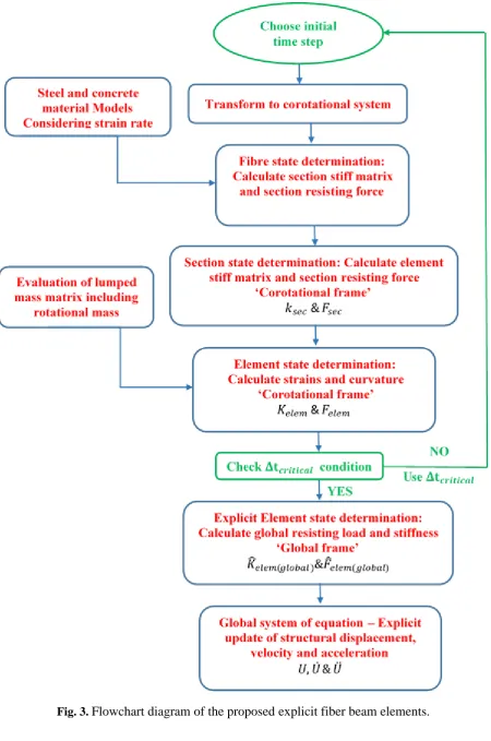
A flowchart diagram summarizing the algorithm of the proposed explicit fiber beam elements

is shown in Fig. (3).

COMPUTATION OF THE MASS MATRIX

The formulation of the developed elements requires that a mass matrix be constructed. A

diagonal mass matrix based on direct lumping should be used to make the inversion of the

mass matrix trivial. All diagonal terms of the lumped mass matrix have to be defined, as

shown in Fig. (4), including a rotational mass.

To evaluate the mass matrix due to self-weight of a beam with element length 𝐿, cross section

area 𝐴 and a uniform mass density 𝜌:

The translational nodal masses in both horizontal and vertical directions = 1₂ 𝜌𝐴𝐿 (39)

The rotational mass at each node = 𝛼𝜌Α𝐿3 (40)

Where from Felippa (2013) the value of 𝛼 varies between 0 and 1/100. If the 𝛼 value is taken

as zero this lead to a singular mass matrix, which cannot be used in an explicit formulation.

16

For the presented elements, the value of 𝛼 was taken equal to (3.5 100⁄ ) and was found to

yield stable and accurate results for the displacement and the force based explicit elements.

Whereas, for the implicit analysis, the value of 𝛼 can be taken equal to zero.

In addition, external masses supported by the element can be lumped at the element ends.

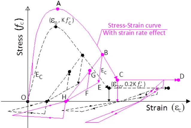
CONCRETE AND STEEL MATERIAL MODELS

The concrete uniaxial material model used by the fiber beam element is based on the Kent

and Park (1971) constitutive law as extended by Scott et al. (1982), while considering the

strain rate effect (Fig.5). The stress-strain curve of concrete captures the nonlinear relation

between the stress and strain and takes into account the effect of the confinement of concrete,

the hysteretic behavior under cyclic loading and the effect of tension stiffening. The

reinforcing steel model adopted by the fiber beam element is based on the Menegotto and

Pinto (1973) constitutive law, as modified by Filippou et al. (1983) to account for isotropic

hardening. The model considers the Bauschinger effect and the strain hardening effect as

shown in Fig. (6). In the proposed element, strain rate effects are also accounted for in the

material models.

To consider the strain rate effect in the material models, the material parameters of the

concrete and steel were modified using the dynamic amplification factor (DAF). The DAF is

a non-dimensional parameter and is used to present the difference between the properties of

the materials under static and dynamic loading. The DAF can be applied to the concrete and

steel material parameters to reflect the strain rate effect.

For the concrete, the value of the concrete compressive strength, the concrete strain at

maximum strength and the concrete tensile strength are amplified, and for the steel

17

The following equations retrieved from the literature were used in the material model. For

normal concrete, the dynamic compressive strength was determined by Fujikake et al.

(2009):

𝑓′𝑐𝑑= 𝑓′𝑐(_𝜀̇𝜀̇

𝑠)

0.006[log 𝜀̇ 𝜀̇⁄ 𝑠𝑡]1.05

𝑓𝑜𝑟 𝜀̇ ≥ 𝜀̇𝑠𝑐 (41)

And the strain corresponding to the dynamic compressive strength was calculated as:

𝜀′𝑐𝑑 = 𝜀′𝑐(_𝜀̇𝜀̇

𝑠)

−0.036+0.01 log (𝜀̇/𝜀̇𝑠𝑡)

𝑓𝑜𝑟 𝜀̇ ≥ 𝜀̇𝑠𝑐 (42)

Where:

𝑓′𝑐𝑑= The dynamic concrete compressive strength at strain rate 𝜀̇ in MPa.

𝑓′_𝑐 = The static compressive strength in MPa.

𝜀′_𝑐𝑑 = The dynamic strain corresponding to𝑓′_𝑐𝑑.

𝜀′_𝑐 = The static strain corresponding to𝑓′_𝑐.

𝜀̇𝑠𝑐 = 1.2 × 10−5.

For the dynamic tensile strength of normal concrete, the Ross et al. (1989) equation was

used:

𝑓_𝑡𝑑 = 𝑓_𝑡exp [0.00126 (log_10𝜀̇𝜀̇

𝑠𝑡)

3.373

] 𝑓𝑜𝑟 𝜀̇ ≥ 𝜀̇_𝑠𝑡 (43)

Where:

𝑓_𝑡𝑑 = The dynamic concrete tensile strength at strain rate 𝜀̇.

𝑓_𝑡 = The static concrete tensile strength.

18

To consider the effect of fiber reinforced concrete on the DAF, the Lok and Zhao (2004)

equations were employed. They used the Split Hopkinson pressure bar in the development of

the strain rate tests that ranged between 20 and 100 s-1 and proposed two equations to express

the compressive response of steel fiber-reinforced concrete subjected to different strain rates

as follow:

𝐷𝐴𝐹 = 1.080 + 0.017 log(𝜀̇) 0 ≤ 𝜀̇ ≤ 20 𝑆−1 ₍₄₄₎

𝐷𝐴𝐹 = 0.067 + 0.796 log(𝜀̇) 20 ≤ 𝜀̇ ≤ 100 𝑆−1 ₍₄₅₎

For the reinforcing steel, and according to Limberger et al. (1982) and Ammann et al.

(1982) the steel elastic modulus 𝐸𝑆 and the strain hardening modulus 𝐸𝑆𝑃 are not affected by

the loading rates. So in the steel material model, only the effect on the yield strength is

considered. The dynamic yield strength 𝑓_𝑠𝑦𝑑 at strain rate 𝜀̇ is estimated by the Malvar (1998) equations. Malvar (1998) studied the strength enhancement of steel reinforcing bars

under the effect of high strain rates and proposed a formula to approximate the straight line

on the logarithmic scale of the dynamic increase factor versus the strain rate.

The equations were derived and are valid for a yield stress fy that ranges between 290 and 710

MPa and are as follows:

𝐷𝐴𝐹 = (₁₀𝜀̇₋₄)𝛾 (46)

For yield stress calculation: 𝛾 = 𝛼_𝑓𝑦; 𝛼_𝑓𝑦 = 0.074 − 0.04(𝑓_𝑦⁄414) (47)

For ultimate stress calculation: 𝛾 = 𝛼_𝑓𝑢 ; 𝛼_𝑓𝑢 = 0.019 − 0.009(𝑓_𝑦⁄414) (48)

Where:

𝜀̇ ∶ The strain rate is in s-1.

19

VALIDATION OF THE NUMERICAL MODEL FOR IMPACT PROBLEMS

Instrumented drop weight tests are widely used to evaluate the response of reinforced

concrete members under impact loads. Hrynyk and Vecchio (2014) used a drop-weight

machine to test intermediate-scale slabs under impact loading. Saatci and Vecchio (2009)

tested several reinforced concrete beams using the drop weight test and validated their

numerical model. Fujikake et al. (2009) also used the same method to impact reinforced

concrete beams and compared their results with analytical methods.

In this research, two experiments from the literature are used to validate the developed fiber

beam finite elements that use the explicit time integration method. In the selected

experiments, instrumented drop weight impact tests were used to examine the dynamic

behavior of doubly reinforced concrete beams and steel fiber-reinforced concrete beams.

- First experiment: Impact Behavior of Reinforced Concrete Beams

An instrumented experimental program was carried out by Saatci and Vecchio (2009) where

eight reinforced concrete beam specimens were tested under free-falling drop-weights. All

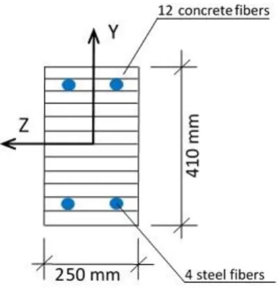
the specimens had a section of 250 mm x 410 mm and a total length of 4880 mm. The beams

were simply supported with a clear span of 3000 mm. All the specimens were doubly

reinforced with equal top and bottom reinforcement that consist of 4 bars with diameter 29.9

mm and a yield stress of 464 MPa. Fig. (7) illustrates the impact test setup used in the

experiment.

For specimen SS3a-1, the drop-weights impacted the specimen once at the mid span, from a

clear height of 3.26 m, with a small drop weight (211 kg). A flexural failure mode was

20

the mid span. However, shear cracks also developed under the impact test mainly after other

multiple impacts.

Specimen SS3a-1 was chosen to be modelled with the fiber beam elements. The Specimen

had a compressive strength of 46.7 MPa and a strain at peak compressive strength equal to

2.51 × 10−3_{. The strain rate effect in this sample was small and didn’t change the material}

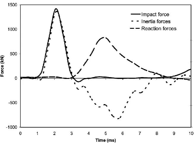
properties much. Fig. (8) displays the impact force and the reaction forces obtained from the

experiment. In the finite element models, each element was divided into 5 sections and the

sections were further divided into 12 concrete fibers and 4 steel fibers (Fig. 9).

A convergence study is first performed for the explicit displacement-based element. The

beam was modelled with 10, 14, 18 and 22 elements including the cantilever parts. Fig. (10)

shows that 18 explicit-based elements were sufficient to reach convergence.

So for the displacement based elements, the beam was subdivided into 18 finite elements.

Regarding the displacement based implicit element a step of 0.01 was adopted while for the

displacement based explicit element a step of 0.01 was unstable and a smaller step of

0.001was used. The impact load was applied in the middle of the beam under force control

and the displacement time history was compared with the experimental results.

Similarly, for the force based elements, the beam was divided into 12 elements to reach

convergence. The same time steps used with the displacement based element were also used.

Fig. (11) shows the midpoint displacement vs time response retrieved from the explicit and

implicit displacement and force based elements. Both four elements produced similar results.

21

The displacement based implicit element performed on average 4 global iterations in every

step to reach convergence. While the force based implicit element performed on average 2

internal iterations and 4 global iterations in every step to reach convergence.

For the fully explicit force based element, the element is initially assigned a large time step of

0.01 and the behavior of the element was monitored as follow:

First it was found that the element was facing stability problems from an early stage. For the

solution for time steps between 0 and 0.04 sec, the largest ∑ 𝐹 3_{1 𝑢𝑛𝑏𝑎𝑙𝑎𝑛𝑐𝑒𝑑}∙Δq ranged between (1.30E-06 and 2.74E-05) and element residual deformations 𝑅 ranged between

0.3E-7 and 0.6E-5. For the largest value of ∑ 𝐹 3_{1 𝑢𝑛𝑏𝑎𝑙𝑎𝑛𝑐𝑒𝑑}∙Δq = 2.74E − 05, using Equation (37) and assuming a tolerance value of 1.00E − 05:

Δt_{𝑐𝑟𝑖𝑡𝑖𝑐𝑎𝑙} 𝑛𝑒𝑤 = 0.01 × √1.00E−05 _2.74E−05 = 0.00604 𝑠𝑒𝑐 (which is the minimum Δt_{𝑐𝑟𝑖𝑡𝑖𝑐𝑎𝑙} of the

12 elements). This new time step was used in the analysis to avoid internal element iterations.

For the rest of the time steps, ∑ 𝐹 3_{1 𝑢𝑛𝑏𝑎𝑙𝑎𝑛𝑐𝑒𝑑}∙Δq ranged between (-0.23E-05 and 0.10E-02):

Δt_{𝑐𝑟𝑖𝑡𝑖𝑐𝑎𝑙} 𝑛𝑒𝑤 = 0.01 × √_0.10E−02 1.00E−05 = 0.001 sec

Using the new time step 0.001, the element didn’t perform any internal iterations and the

element residual deformations 𝑅 ranged between 0.10E-30 and 0.10E-10, satisfying

convergence.

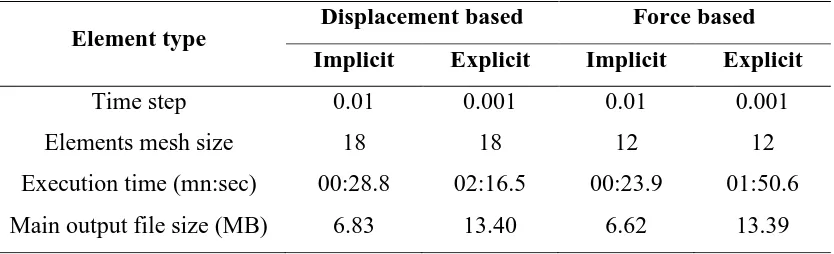
Table 1 shows the execution time each element used to solve the problem and the size of the

main output file. From the table, it can be observed that because implicit elements use larger

22

case), and smaller output files. The elimination of the iterations did not save time as the

selected time step played the major role in determining the execution time. Further, the

explicit force based element required a smaller execution time than the explicit displacement

based element mainly because a coarse mesh was adopted. This experiment confirmed the

ability of the explicit elements in modelling the impact behavior of reinforced concrete beams

while avoiding internal and external element iterations.

Table 1. Comparison between execution time of the implicit and the explicit displacement and force based elements for sample SS3a-1.

- Second experiment: Impact response of reinforced concrete beam

Fujikake et al. (2009) tested several reinforced concrete (RC) beams under impact loadings

using a drop hammer impact test. Fig. (12) shows the drop hammer impact test setup used in

the experiment. The beams were designed to allow for an overall flexural failure. The authors

also used an analytical model that consists of a two-degree-of-freedom mass-spring-damper

system to simulate the RC beams analytically. The system consisted of one degree of

freedom to express the local impact response between the drop weight and the beam and

Element type Displacement based Force based

Implicit Explicit Implicit Explicit

Time step 0.01 0.001 0.01 0.001

Elements mesh size 18 18 12 12

Execution time (mn:sec) 00:28.8 02:16.5 00:23.9 01:50.6

23

another one to express the overall response of the beam. The analysis technique involved the

determination of the moment-curvature relationship of the beam using section by section

analysis procedure whereas the strain rate effects were considered. Then the calculation of the

load-midspan deflection relationship using the moment-curvature relationship was

performed.

The two Specimens S1616-A and S1616-D were chosen to be modelled with the fiber beam

elements. The RC beam specimens had a rectangular cross section of 250x150 mm and a total

span length of 1400 mm. The beams were simply supported at their ends and were allowed to

freely rotate while preventing them from moving out of plane. The beams were reinforced

with 2Ø16 top and bottom bars with yield strengths of 426 MPa. The concrete compressive

strength was 42 MPa.

The impact forces applied in the middle of the beams retrieved from the experiment are

shown in Fig. (13) for sample S1616-A and Fig. (14) for sample S1616-D. Both the implicit

and explicit fiber beam elements were used to simulate the behavior of the two beams under

the impact force. Due to symmetry, only half of the beams were modelled with a variable

number of elements. The beam in this problem was assumed simply-supported, which allows

for free rotation at the ends while preventing vertical displacements; and symmetry was

respected in the middle by allowing vertical movement and preventing horizontal movement

and rotations. Consequently no second order effect is expected in this case.

Each element was divided into five sections and each section was further divided into 12

concrete fibers and 4 steel fibers that represent the top and bottom reinforcement (Fig. 15).

The drop hammer used had a mass of 400 kg and was dropped freely onto the top surface of

24

was the smallest with 0.15m and for specimen S1616-D the drop height was the highest with

1.2m.

A laser displacement sensor was used to measure the midspan deflection of the beam and a

dynamic load cell was utilized to measure the contact force between the hammer and the

beam.

Specimen S1616-A

The impact force time history was used as input for the two fiber beam elements. This was

retrieved from the experiment. In the implicit model, the step size was chosen as 0.001 sec

and an excessive maximum of 20 iterations per step was allowed (although usually 4 to 8

iterations are commonly sufficient). The total number of steps was 2500. In the explicit

force-based model, the time step size was chosen as 0.00001 to satisfy ∆𝑡_𝑚𝑖𝑛 and Δt𝑐𝑟𝑖𝑡𝑖𝑐𝑎𝑙 based on

a fully explicit element with no iteration and a required tolerance of 1.00E − 06, thus 250000

steps were used.

For the proposed criteria of the force based explicit model, the element was first assigned a

large time step of 0.001, and the behavior of the element is monitored below:

The element worked well at the initial stage between steps 0 and 0.544

sec, ∑ 𝐹 3_{1 𝑢𝑛𝑏𝑎𝑙𝑎𝑛𝑐𝑒𝑑}∙Δq ranged between (0.12E-46 and 0.83E-30) and the element residual deformations R ranged between 0.2E-14 and 0.7E-29.

Then from steps 0.544 to 1.23 sec, the largest ∑ 𝐹 31 𝑢𝑛𝑏𝑎𝑙𝑎𝑛𝑐𝑒𝑑∙Δq ranged between

25

For the largest value of ∑ 𝐹 3_{1 𝑢𝑛𝑏𝑎𝑙𝑎𝑛𝑐𝑒𝑑}∙Δq = 1.26E − 06 and, using equation (37) with a

tolerance value of 1.00E − 06, Δt_{𝑐𝑟𝑖𝑡𝑖𝑐𝑎𝑙} 𝑛𝑒𝑤= 0.001 × √1.00E−06 _0.95E−05 = 0.00032 𝑠𝑒𝑐. This

new time step ensured no element iterations are performed.

Later, between time steps 1.23 sec and the end of the analysis, ∑ 𝐹 3_{1 𝑢𝑛𝑏𝑎𝑙𝑎𝑛𝑐𝑒𝑑}∙Δq ranged between (0.50E-02 and 0.44E-07)

Thus Δt𝑐𝑟𝑖𝑡𝑖𝑐𝑎𝑙 𝑛𝑒𝑤= 0.001 × √1.00E−06 _0.50E−02 = 0.000014 sec

Using a new time step of 0.000014 sec, the element didn’t perform any internal iterations and

𝑅 ranged between 0.10E-30 and 0.10E-16.

For the explicit displacement-based model, the time step size was chosen as 0.0001 to

fulfil the ∆𝑡_𝑚𝑖𝑛 requirement. A diagonal lumped mass was adopted for the explicit analysis.

The material constitutive parameters used in the finite element model considering the strain

rate effect were taken as follow:

𝑓′_𝑐𝑑= 52 MPa, 𝜀′_𝑐𝑑 = 0.009, 𝑓_𝑡𝑑 = 3 MPa and 𝑓_𝑠𝑦𝑑 = 580.0 𝑀𝑃𝑎.

With only two elements, the two explicit models were able to follow the input load-time

curve and to predict the displacement-time history accurately as shown in Fig. (16). On the

other hand, both of the implicit models, the displacement and force elements, suffered from

severe convergence issues and resulted in unstable behavior and inaccurate displacement

estimates (Fig. 16). It is worth mentioning that both explicit elements converged with only

two elements as the impact load was small for this specimen. Fig. (17) shows the bending

moment distribution along the span of beam S1616-A at the maximum displacement using

the explicit force based element. Due to the assumption of the force-based formulation, the

26

The difference between the capabilities of the explicit and implicit elements is very clear in

this problem, which emphasises the superiority of the explicit time integration methods for

short time duration impact problems. It should be noted that the explicit force-based element

requires a higher number of time steps in case no internal element iterations is allowed when

compared with the mixed explicit implicit force-based element or the explicit

displacement-based element.

Specimen S1616-D

For the implicit model, the step size was also chosen as 0.001 and the total number of steps

was 3500. In the explicit force-based model, the time step size was initially chosen as

0.00001 based on a fully explicit element with no iteration at all and a tolerance of 1.00E −

06, thus 350000 steps were used. For the explicit displacement-based model, the time step

size was chosen the same as the one used to solve specimen S1616-A. A diagonal lumped

mass was created for the explicit element.

For the material parameters, the values considering the strain rate effect were taken as follow:

𝑓′𝑐𝑑= 44.0 MPa, 𝜀′𝑐𝑑 = 0.0950, 𝑓𝑡𝑑 = 1.0 MPa and 𝑓𝑠𝑦𝑑 = 430.0 𝑀𝑃𝑎.

As seen in Fig. (18), only the two explicit models were able to predict the behavior of the

impact problem to a good extent with four elements for the force-based and eight elements

for the displacement-based approach. Both of the implicit models, the displacement and force

elements, failed to follow the input path and produced exaggerated deflection values. The two

fiber beam elements overcome the complexity of the analysis method used by Fujikake et al.

(2009). Further, the force-based explicit element produced better results than the

displacement-based explicit element as it requires less number of elements to reach

27

the maximum displacement using the explicit force based element. It also confirms the linear

distribution of the moment function.

The ability of the implicit element to solve short term dynamic problems is limited and is due

to several factors including the impact force value, the load input path complication, the

duration of the load and the nonlinear material behavior. On the other hand, the use of

explicit techniques with the fiber beam element is an advanced method to solve highly

nonlinear dynamic problems without the need for iterations and convergence complications.

The elements benefit from their simplicity which makes them competitive with complex

continuum elements available in commercial finite element software.

CONCLUSION

In this paper, two plane fiber beam elements are presented that adopt an explicit time

integration scheme to solve short-term dynamic problems, particularly impact problems

where a high force is applied over a very short duration. The elements can be used reliably to

analyse different reinforced concrete structures to ensure their safety against impact loading.

The elements use a displacement-based and a force-based formulation respectively, and

benefit from advanced material models that can simulate the nonlinear behavior of concrete

and steel materials. The developed elements overcome the difficulties and complications that

are accompanied with the implicit time integration method, such as the need to iterate in

every time step and the convergence requirements. Yet, the explicit element necessitates the

use of a diagonal lumped mass matrix and the chosen time increment has to be smaller than

the stable time increment required to maintain the stability of the numerical solution.

Additionally for the fully explicit force-based element, a single iteration can be used if

28

particularly the force-based element, represent a simple yet powerful tool for analysis of

complex impact problems efficiently while using a limited number of finite elements.

The results of the two plane elements were compared with experimental tests of impact

problems in order to validate their accuracy, and promising outcomes were obtained.

Future work will attempt to expand the current formulation to the three-dimensional space

including second order and shear deformation effects. Analysis under blast loads will be

evaluated.

29 REFERENCES

Alemdar, B. and White, D. (2005). "Displacement, Flexibility, and Mixed Beam–Column

Finite Element Formulations for Distributed Plasticity Analysis." J. Struct. Eng., 131(12),

pp.1811-1819.

Ammann, W., Muehlematter, M., & Bachmann, H. (1982). "Stress-strain behaviour of non

prestressed and prestressed reinforcing steel at high strain rates." Proc. of

RILEM-CEB-IABSE-IASS, Concrete structures under impact and impulsive loading, p. 656, Berlin,

BAM

Bathe, K. and Cimento, A. (1980). "Some practical procedures for the solution of nonlinear

finite element equations." Computer Methods in Applied Mechanics and Engineering,

22(1), pp.59-85.

Chang, S. (2009). "An explicit method with improved stability property." International

Journal for Numerical Methods in Engineering, 77(8), pp.1100-1120.

Chen, L., Xiao, Y., and El-Tawil, S. (2016). "Impact Tests of Model RC Columns by an

Equivalent Truck Frame." J. Struct. Eng., 10.1061/(ASCE)ST.1943-541X.0001449,

04016002.

Felippa, C. (2013). "Matrix Finite Element Methods in Dynamics (Course in Preparation)."

1st ed. [ebook] Colorado, Chapter 18.

<http://www.colorado.edu/engineering/CAS/courses.d/MFEMD.d/MFEMD.Ch18.d/MFE

MD.Ch18.pdf> (Dec. 6, 2016).

Filippou, F.C., Popov, E.P., and Bertero, V.V. (1983). "Effects of Bond Deterioration on

Hysteretic Behavior of Reinforced Concrete Joints." Report No. UCB/EERC-83/19,

30

Fujikake, K., Li, B. and Soeun, S. (2009). "Impact Response of Reinforced Concrete Beam

and Its Analytical Evaluation." Journal of Structural Engineering, 135(8), pp. 938-950.

Fulei, W. and Yungui, L. (2011). "A Nonlinear Dynamic Beam Element with Explicit

Algorithms." Communications in Computer and Information Scienc, CCIS 163, pp.

311-318.

Gu, L. and Wu, S. (2013). "Introduction to the explicit finite element method for nonlinear

transient dynamics". Hoboken, N.J.: Wiley, p.5.

Hong, S.G., Lee, S.J. and Lee, M.J. (2014). "Steel plate concrete walls for containment

structures in Korea: in-plane shear behavior." Infrastruct Syst Nucl Energy, pp. 237–257

Hrynyk, T. and Vecchio, F. (2014). "Behavior of Steel Fiber-Reinforced Concrete Slabs

under Impact Load." ACI Structural Journal, 111(5).

Huang, C. and Wu, T. (2009). "A study on dynamic impact of vertical concrete cask tip-over

using explicit finite element analysis procedures." Annals of Nuclear Energy, 36(2), pp.

213-221.

Kent, D.C., and Park, R. (1971). "Flexural Members with Confined Concrete." Journal of the

Structural Division., ASCE, Vol. 97, No ST7, pp. 1969-1990.

Kujawski, J. (1988). "Stable semi-explicit algorithms for non-linear dynamic problems."

Earthquake Engineering & Structural Dynamics, 16(6), pp. 855-865.

Limberger, E., Brandes, K., & Herter, J. (1982). "Influence of mechanical properties of

reinforcing steel on the ductility of reinforced concrete beams with respect to high strain

rates." In Plauk, G. (Ed.). Concrete structures under impact and impulsive loading, p. 656.

Germany

Lok, T. and Zhao, P. (2004). "Impact Response of Steel Fiber-Reinforced Concrete Using a

31

Malvar, L. (1998). "Review of Static and Dynamic Properties of Steel Reinforcing Bars."

ACI Materials Journal, 95(5), pp. 609-616.

Menegotto, M., and Pinto, P.E. (1973). "Method of Analysis for Cyclically Loaded

Reinforced Concrete Plane Frames Including Changes in Geometry and Nonelastic

Behavior of Elements under Combined Normal Force and Bending." IABSE Symposium

on Resistance and Ultimate Deformability of Structures Acted on by Well-Defined

Repeated Loads, Final Report, Lisbon.

Miranda, I., Ferencz, R. and Hughes, T. (1989). "An improved implicit-explicit time

integration method for structural dynamics." Earthquake Engineering & Structural

Dynamics, 18(5), pp. 643-653.

Mullapudi, T. and Ayoub, A. (2010). "Modeling of the seismic behavior of shear-critical

reinforced concrete columns." Engineering Structures, 32(11), pp. 3601-3615.

Neuenhofer, A. and Filippou, F. (1997). "Evaluation of Nonlinear Frame Finite-Element

Models." Journal of Structural Engineering, 123(7), pp.958-966.

Pezeshk, S. and Camp, C. (1995). "An explicit time integration technique for dynamic

analyses." International Journal for Numerical Methods in Engineering, 38(13), pp.

2265-2281.

Ross, C.A., Thompson, P.Y., Tedesco, J.W., (1989). "Split-hopkinson pressure-bar tests on

concrete and mortar in tension and compression." ACI Mater. J. 86 (5), pp. 475–481.

Saatci, S. and Vecchio, F. (2009). "Effects of Shear Mechanisms on Impact Behavior of

Reinforced Concrete Beams." ACI Structural Journal, 106(1).

Scott, B.D., Park, R., and Priestley, M.J.N. (1982). "Stress-Strain Behavior of Concrete

Confined by Overlapping Hoops at Low and High Strain Rates." ACI. Journal, Vol. 79,

32

Spacone, E., Filippou, F. and Taucer, F. (1996). "Fibre beam-column model for non-linear

analysis of r/c frames: part i. formulation." Earthquake Engineering & Structural

Dynamics, 25(7), pp.711-725

Sun, J., Lee, K. and Lee, H. (2000). "Comparison of implicit and explicit finite element

methods for dynamic problems." Journal of Materials Processing Technology, 105(1-2),

pp.110-118.

Taylor, R. (2014). FEAP - Finite Element Analysis Program. Berkeley: University of

California.

Tenek, L. (2015). "A Beam Finite Element Based on the Explicit Finite Element Method."

International Review of Civil Engineering (IRECE), 6(5), p. 124.

Yang, D., Jung, D., Song, I., Yoo, D. and Lee, J. (1995). "Comparative investigation into

implicit, explicit, and iterative implicit/explicit schemes for the simulation of sheet-metal

forming processes." Journal of Materials Processing Technology, 50(1-4), pp.39-53.

Yoshida, Y., Masuda, N., Morimoto, T. and Hirosawa, N. (1980). "An incremental

formulation for computer analysis of space framed structures." Journal of Structural

33 LIST OF FIGURE CAPTIONS

Fig. 1. Time integration graph.

Fig. 2. Element nodal forces and degrees of freedom in the corotational frame.

Fig. 3. Flowchart diagram of the proposed explicit fiber beam elements.

Fig. 4. Direct mass lumping for two-node plane beam element.

Fig. 5. Concrete material model with and without strain rate effect.

Fig. 6. Menegotto-Pinto Cyclic stress-strain curve of mild steel bar with and without strain

rate effect.

Fig. 7. Test setup of the beams, figure from (Saatci and Vecchio 2009).

Fig. 8. Impact and reaction forces vs time for sample SS3a-1, figure from (Saatci and

Vecchio 2009).

Fig. 9. Fiber beam element cross section mesh for sample SS3a-1.

Fig. 10. Conversion study for the explicit displacement base element using sample SS3a-1.

Fig. 11. Midpoint displacement time history of sample SS3a-1.

Fig. 12. Drop hammer impact test setup, figure from (Fujikake et al. 2009).

Fig. 13. Impact load history for sample S1616-A, figure from (Fujikake et al. 2009).

Fig. 14. Impact load history for sample S1616-D, figure from (Fujikake et al. 2009).

Fig. 15. Fiber beam element cross section mesh for sample S1616-A and S1616-D.

Fig. 16. Deflection time history for specimen S1616-A.

Fig. 17. Bending moment at maximum displacement using the explicit force based element

(specimen S1616-A).

Fig. 18. Deflection time history for specimen S1616-D.

Fig. 19. Bending moment at maximum displacement using the explicit force based element

34

35

Fig. 2. Element nodal forces and degrees of freedom in the corotational frame.

X

Y

Z

L

36

37

38

39

40

41

42

43

44

45

46

47

48

49

50

Fig.17. Bending moment at maximum displacement using the explicit force based element

51

52

Fig.19. Bending moment at maximum displacement using the explicit force based element