Initial state prediction in planning

Initial State Prediction in Planning

Senka Krivic,

Michael Cashmore,

Bram Ridder,

Daniele Magazzeni,

_{Sandor Szedmak,}

_{Justus Piater}

1_{Department of Computer}

Science, University of Innsbruck, Austria

2_{Department of Computer}

Science, King’s College London, United Kingdom

3_{Department of Computer}

Science, Aalto University, Finland

fi[email protected] fi[email protected] sandor.szedmak@aalto.fi

Abstract

While recent advances in offline reasoning techniques and online execution strategies have made planning under uncer-tainty more robust, the application of plans in partially-known environments is still a difficult and important topic. In this paper we present an approach for predicting new information about a partially-known initial state, represented as a multi-graph utilizing Maximum-Margin Multi-Valued Regression. We evaluate this approach in four different domains, demon-strating high recall and accuracy.

1

Introduction

Planning in many domains means planning with incomplete and uncertain information. In such domains plans generated can be fragile. Contingency planning (Bonet and Geffner 2000; Hoffmann and Brafman 2005), conformant planning (Smith and Weld 1998; Palacios and Geffner 2006), and replanning techniques (Brafman and Shani 2014) work to make execution more robust, for an acceptable cost of com-putational difficulty or plan quality.

In this paper we focus on the problem of planning with incomplete information on the initial state in a deterministic domain. We describe a preprocessing step that predicts new information about a partially-known initial state inspired by research onassociative learning(Hill 1984).

Humans associate certain holidays with specific sounds and smells, or foods with specific flavours, colours and tex-tures. Pavlov and Anrep (Pavlov and Anrep 2003) have shown that it is possible to pair an unconditioned stimulus with another previously neutral stimulus. This makes it pos-sible to learn and predict events in terms of associations be-tween stimuli, representing the paradigm ofClassical con-ditioning.

The idea is related to that ofassumption-based planning (ABP) (Sammy Davis-Mendelow 2013), which formalises the idea of planning in a partially unknown initial state with assumptions. Davis-Mendelow et al. show that ABP has great utility for tasks that share a computational core with planning, and encapsulates a compelling for of com-mon sense planning.

Copyright c2017, Association for the Advancement of Artificial Intelligence (www.aaai.org). All rights reserved.

In this paper we present a novel way in which to make such assumptions, focusing on domains in which a robotic agent has to make fast decisions. For example scenarios such as the robocub where the robot has a partial information of the initial state and has to make fast decisions, or an au-tonomous underwater vehicle that must make critical deci-sions before its position drifts.

We demonstrate that it is possible to predict missing infor-mation in an initial state by exploiting the similarities among known facts. We pose the problem of prediction as that of learning missing edges in a graph. The learned edges are analogous to assumptions about facts within the initial state. To solve this associative learning problem we use a kernel-based approach for learning missing edges in a partially-given multigraph (Krivic et al. 2015). This allows us to prop-agate knowledge from existing relations to unknown rela-tions in a partially-known initial state.

Maximum Margin Multi-Valued Regression (M3_{V R )} (Ghazanfar, Pr¨ugel-Bennett, and Szedmak 2012; Szedmak, Ugur, and Piater 2014) is applied to the class of learning problems where item-item relations might be given by dif-ferent attributes. This learning framework is used at the core of a recommender system (Ghazanfar, Pr¨ugel-Bennett, and Szedmak 2012) and for predicting the effects of an action on pairs of objects in an affordance learning prob-lem (Szedmak, Ugur, and Piater 2014). Their results show that it can deal with sparse, incomplete and noisy infor-mation. The M3

V R is compared with the state-of-the-art methods and is an established and competitive method for prediction of missing relations and recommender based systems (Ghazanfar, Pr¨ugel-Bennett, and Szedmak 2012; Krivic et al. 2015).

Krivic et al. (2015) use this method to refine a world model for planning to tidy up a child’s room with a robotic agent. The system is used to learn the edges describing the possible spatial relations between objects. We build on this, describing how the approach can be generalised for use in any planning domain, learning edges that correspond to generic propositions in the initial state. In particular we describe: how the initial state is represented as a partially-known multigraph; the approach for learning missing edges; how the results of the learning framework are translated back into the planning domain; and finally, how they can be used in the planning process.

The AAAI-17 Workshop on

The problem is similar to a restricted class of contingency planning problems with deterministic actions, partially observable Markov decision processes (POMDP) (Bonet 2009). Techniques exist to solve these problems by first converting them into classical planning problems: K -Planner (Bonet and Geffner 2011), PO-RPR (Muise, Belle, and McIlraith 2014), and CLG (Albore and Geffner 2009); or using conformant planning techniques (Smith and Weld 1998; Palacios and Geffner 2006). Our work differs in that we do not translate the whole problem, but instead remove uncertainty by making predictions. In our problem there is no known probability distribution over the existence of propositions in the partially-known initial state. Moreover, the approach is orthogonal in that uncertainty is removed from the problem through prediction, either enabling a de-terministic solution, or simplifying the contingency planning problem should they be used in combination.

By integrating the learning framework into a planning and execution system we demonstrate its efficacy on several do-mains. We perform an empirical evaluation on a range of problems in these domains. We show that:

• With already20%knowledge of the initial state the accu-racy of complete initial state prediction is90%.

• Prediction leads to plans that are more robust (fewer re-plans are required) compared to an optimistic classical planning approach.

• Comparing with CLG, prediction increases the scalability of contingency planning, at a cost to robustness.

In Section 2 we describe our problem formulation for learning new relations in partially-known initial states. We describe the learning problem in Section 3, and explain how the learning framework is used to solve the formulated prob-lem. In Section 4 we perform an evaluation. We conclude in Section 5.

2

Predictions in the Planning Problem

Definition 1 (Planning Problem) A planning instanceΠis a pair_{Dom, P rob}, where_Dom = _{P s, As, arity}is a tuple consisting of a finite set of predicate symbolsP s, a finite set of (durative) actions As, and a function arity map-ping all symbols inP sto their respective arities. The triple P rob=Ob, Init, Gconsists of a finite set of domain ob-jects Ob, the partial initial state Init, and the goal specifica-tion G.

The atoms of the planning instance are the (finitely many) expressions formed by grounding – applying the predicate symbols P sto the objects in Ob (respecting arities). The resultant expressions are the set of propositionsP.

A statesis described by a set of literals formed from the propositions inP,{lp,¬lp,∀p ∈ P}. If every proposition

fromP is represented by a literal in the state, then we say thatsis acomplete state. Apartial stateis a set of literals s⊂s, wheresis a complete state.

The initial stateinitis a partial state. A partial state can beextendedinto a complete state.

Definition 2 (Extending a Partial State) Let _s be a par-tial state of Planning problemΠ. Extending the state_s is a function _Extend(Π_{, s}) : _s → _swhere_sis a complete state ands ⊂s.

We describe a pre-processing step implementingExtend. All unknown propositional values in a partially-known ini-tial state are predicted, producing a complete iniini-tial state. Briefly, the functionExtend(Π, s)is implemented as fol-lows: the initial state init is converted into a multigraph; edges in the multigraph are learned usingM3

V R; then the new edges are added as literals to the initial state.

First we describe the construction of the multigraph, then in Section 3 we describe the relational problem, and then how the learned relations are inserted back into the initial state. Finally, the complete initial state can be used by a clas-sical planner to generate a plan.

Constructing the Multigraph

We represent a partially-known initial state init as a partially-known multigraphM.

Definition 3 (Partially-known Multigraph) A partially-known Multigraph_M is a pair_{V, E}, where_V is a set of vertices, andEa set of values of labelled, directed edges.

The values assigned to all possible edges are{0,1,?} cor-responding to{not-existing,existing,unknown}. We useE to denote a set of edges values in a partially-known multi-graph, whileE denotes the set of edges values in a com-pleted multigraph. The partial state init is described as a partially-known multigraph with an edge for each proposi-tionp∈Pthat is either unknown or known to be true. That is:

V ≡ Ob

E = {epred(b, u)|(b, u)∈V ×V}

The existence of adirected edgeepred(b, u)between two

verticesbandufor a predicatepredis described by the func-tionLpred : V ×V → {0,1,?}. For example, letbandu

be two vertices in setV. For propositionpinvolving objects bandu,Lpred(b, u) = 0if¬lp ∈init,Lpred(b, u) = 1if

lp ∈init, andLpred(b, u) =?otherwise. Known edges are

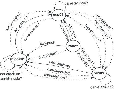
denoted with solid lines and unknown ones with dashed line such as in Figure 1. Edges are directed in the order the object symbols appear in the proposition. In the following we use B andU to differentiate between vertices of outgoing and incoming edges respectively. In our problemB=U =V.

Example

Figure 1: The graphM representing the initial state in the example problem. Solid edges correspond to propositions known to be true,Lpred(b, u) = 1. Dashed edges correspond

to propositions whose value is unknown in the initial state, Lpred(b, u) = ?.

(define (domain toy-domain)

(:requirements :strips :typing ...) (:types

waypoint vehicle interactable

box toy - interactable block - toy

gripper)

(:predicates

(connected ?wp1 ?wp2 - waypoint) (at ?v - vehicle ?wp - waypoint) (near ?v - vehicle ?wp - waypoint)

(can-pickup ?r ?interactable) (can-push ?r ?interactable)

(can-stack-on ?interactable ?interactable) (can-fit-inside ?interactable ?box) ...)

(:durative-action goto ... (:durative-action pickup ... (:durative-action putdown ... (:durative-action stack ... (:durative-action unstack ... (:durative-action put_in_box ... )

Figure 2: A fragment of thetoy-domain. Some predicates and the body of operators are omitted for space.

state are assumed to be false. However, in this initial state those literals are assumed to be unknown.

A graphM is generated, the vertices of which areOb:= {robot, cup01, box01, block01}. The graph is shown in fig-ure 1.

(define (problem toy-example-problem) (:domain toy-domain)

(:objects

wp1 wp2 wp3 ... - waypoint robot - vehicle

cup01 ... - interactable box01 ... - box

block01 ... - block )

(:init

(can-pickup robot cup01) (can-push robot block01) (can-push robot cup01) (can-stack-on box01 block01) (can-stack-on block01 cup01) ...)

(:goal ...) )

Figure 3: A fragment of an example problem from the tidy-roomdomain.

3

Predicting Missing Edges in a Multigraph

In this section we describe the procedure of predicting miss-ing edges in a partially-known multigraph. We useM3

V R to extract similarities among vertices based on known edges and to estimate missing edges, embodying the process of as-sociative learning.

M3

V R is a maximum-margin learning framework for predicting incomplete data. The main idea is to capture the hidden structure in the graph. The structure of the graph represents the underlying structure of the environment. De-pending on the regularities which occur in environments, these structures can be less and higher complex. In the ex-ample in figure 1 it is unknown if(robot can-pickup block01). A prediction is made based on the available information about the robotand block01. By observ-ing existobserv-ing relations, one can recognize that block01 and cup01 are similar. Thus it is predicted that robot can-pickup block01istrue.

Generalized, the problem of predicting missing relations is a problem of predicting directed edges from the vertices in a setBto the vertices in a setU. We reconstruct a function f :B×U →Efrom knowledge about existing edges. The functionf describes the mapping of vertices to a complete set of edgesE. In this way, the set of edgesE, representing the known propositions, can be used to measure the simi-larity between the elements of the vertex setV representing the objects. Using this measure of similarity, missing edges, representing unknown predicates, can be predicted.

For an origin vertexband a destination vertexu, we define the vector of edges

ebu={Lpred(b, u)|pred∈P s}

vector:

erobot,block01

= [Lcan−f it−inside(robot, block01),

Lcan−stack−on(robot, block01),

Lcan−push(robot, block01),

Lcan−pickup(robot, block01)]

= [0,0,1,?]

Then, we define the projections of known edgesEinto a set containing origin verticesB and destination verticesU by

B ={b∈B|∃pred∈P s:∀U, Lpred(b, u)=?}

and

U ={u∈U|∃pred∈P s:∀B, Lpred(b, u)=?}

Finally, the learning problem is given by a set of sample items consisting of three elements(b, u,ebu), where(b, u)∈

B×U, ande_bu∈E. To realize this learning task we set up an optimization routine for maximum-margin regression. Since the functionf that defines how edges are assigned to vertices can be very complex, a transformation is applied to both vertices and edges, embedding them into Hilbert spaces1. We assume that:

Condition 1 There exists a mapping_φfrom_Vinto a Hilbert space Hφ, with the kernel function κvertex defined on all possible pairs_B and_U of all subsets of_B×_U such that κvertex(B, U) =φ(B), φ(U).

Condition 2 Similarly there is another mapping ψ of E into a Hilbert space _Hψ with a kernel function_κedge de-fined for all pairs _e1, e2 ∈ E such thatκedge(e1, e2) =

ψ(e1), ψ(e2).

HφandHψare feature representations of the domains of

B,U, andE. The vectorsφ(·)andψ(·)are calledfeature vectors. This allows us to use the inner product as a measure of similarity.

The mapping function can now instead be defined on fea-ture vectors, i.e.,F :Hφ→Hψ. It is indirectly and partially

given by the subsetE. The input for the mapping function F is given by the feature vectors of vertices, and the output is a feature vector of edges. To eachb ∈Brepresenting an origin vertex, we assign such a mappingFb.

Reconstructing these mappings is done by finding a vector-valued function that extendsE to all possible pairs of vertices by exploiting the latent interactions between the edges. For each elementbwe assign a linear operatorWb

which mapsHφtoHψ. Thus predictor functions can be

cre-ated as

ψ(e_bu)←W_bφ(u),(b, u)⊂B∩U (1)

Wbis a tensor representing a linear transformation

project-ing elements ofHφintoHψ, which needs to be learned. The

correlation between the vectorsW_bφ(u)andψ(e_bu)is de-scribed by the inner product ψ(ebu),Wbφ(u)Hψ. If the

1

Hilbert spaces are high dimensional vector spaces with inner product as scalar quantity associated to the each pair of vectors.

correlation betweenW_bφ(u)andψ(ebu)is higher, the inner

product will have a greater value. As a consequenceψ(ebu)

can be predicted by a linear functionW_bφ(u).

Known edges are used to determineWb for each

map-ping. A learner is assigned to learn each mapmap-ping. The num-ber of learners is equal to the numnum-ber of vertices. To exploit the knowledge about existing edges linking different vertices ofB, learners are coupled into one assembly by shared slack variables representing the loss to be minimized by the learn-ers with respect to constraints. Detailed descriptions of the optimization procedure can be found in related work (Krivic et al. 2015; Ghazanfar, Pr¨ugel-Bennett, and Szedmak 2012). In this procedure there are as many constraints as the num-ber of known edges inE. Therefore the complexity of the prediction problem is equal to O(|E|), where|E| stands for the cardinality of the setE.

Once determined, the linear mappings Wb allow us to

make predictions of missing edges for elementsb. The value of the inner product of the edge feature vectorψ(ebu)and

Wbφ(u)can be seen as a measure of confidence in that edge

belonging to a specific class (in this case0or1):

conf{L∗pred(b, u) =c}=

ψ(ebu|L∗pred(b, u) =c),Wbφ(u)_Hψ

wherec ∈ {0,1}, andL∗_pred(b, u)is an unknown value in

ebu∈EEof predicatepred.

For each predictionL∗_pred(b, u), we update the existence of the directed edges:

Lpred(b, u) = arg max

c∈{0,1}

conf{L∗_pred(b, u) =c}

Thus, the graph is completed.

Extending a Partial State with Predictions

Given a complete multigraph, we extend the partially-known initial stateinitby adding literals to the state:

(lp∈init)↔(Lpred(b, u) = 1)

where lp is the positive literal of proposition p, formed

from predicate pred between objects b and u. For exam-ple, Figure 1 contains an edge representing the proposition can-pickup(robot, block01).

Initially, Lpickup(robot, block01) = ?. After prediction,

Lpickup(robot, block01) = 1. Therefore, we add to the

ini-tial state the literal(can pickup robot block01).

4

Evaluation

!"# !

! "#

!"# !#

!" ! "

Figure 4: Accuracy results of 10-fold cross validation obtained by variating number of objects and the known data percentage.

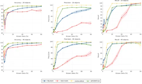
Figure 5: Comparison of accuracy, precision and recall with standard deviation for all 4 domains in case of 20 and 40 objects. Each of the six graphs represents one slice through each of the four graphs of Figure 4, together with standard deviations.

robots are gathering samples; andpersistent-auv, described by Palomeras et al. (2016).

In each domain we generate initial states, varying the size of the problem and percentage of initial knowledge. The size is varied by increasing the number of objects from 5 to 100 by an increment of 5. This increases the number of propositions quadratically. The initial knowledge is varied by generating complete initial states and removing literals at random. The percentage of initial knowledge was varied be-tween 0.5% and 80% (14 values). For each combination of parameters we randomly created 10 instances of a problem utilizing 10-fold cross validation.

The prediction was applied to every problem. The result of the prediction was compared to the ground truth. Figure 4 shows the mean accuracy in each domain. The accuracy is

the number of truly predicted relations as a percentge of all missing relations.

The number of learned relations is large for each domain: for a small percentage of initial knowledge (20%) the over-all accuracy of the process is higher than 90% for most of the problems except for the rovers domain with a number of objects less than 20 (Figure 6). Accuracy increases with the size of the problems. With 40 objects in the each problem domain already 8% of known data is enough for accuracy over 90%.Course-advisorandpersistent-auvdomains con-tain more instances of objects and more predicates compared with the other two domains. This results in larger networks. Thus, for these domains, the accuracy is better for smaller numbers of objects as well.

posi-0 20 40 60 80 100

Number of objects

0 10 20 30 40 50 60

Known Data (%)

tidy-room mars-rovers course-advisor persistent-auv

Figure 6: Minimal percentage of known data which gives stable accuracy equal to or higher than90%.

tive literals (the average ratio is 76:1) we also analysed pre-cision and recall for the category representing positive lit-erals. Precision is the percentage of all literals predicted to be positive which are predicted correctly. Recall is the per-centage of positive literals in the ground truth which were correctly predicted.

We also give a comparison for each domain for 20 and 40 objects in Figure 5. Thecourse-advisor and persistent-auvdomains appear to be simpler than the tidy-room and mars-roversdomains and accuracy is high with a very small proportion of known data. However in thecourse-advisor domain overfitting effects appear for high percentages of known data and many objects (Figures 4 and 5).

With20%of the initial predicates and with 20 objects re-call and accuracy are higher than90%for all domains except mars-rovers. To examine the problem size conditions we ex-tracted from the testing results which amount of the known data is needed to achieve accuraccy higher than 90%. This is shown in the Figure 6. Accuracy increases with the size of the problems. With 40 objects in the each problem domain already 8% of known data is enough for accuracy over 90%. Course-advisor and persistent-auv domains contain more instances of objects and more predicates compared with the other two domains. This results in larger networks. Thus, for these domains, the accuracy is better for smaller numbers of objects as well.The accuracy depends on the structure of used domains, their size and complexity of regularities in re-lations between objects. Results show good predictions for large and small problems with different complexities.

This combination of high accuracy, precision and recall allows us to solve many otherwise unsolvable instances, while maintaining a high degree of robustness. Without pre-processing, no problems could be solved.

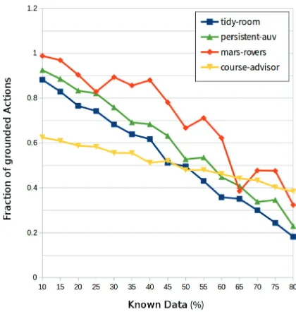
To analyse the effect of prediction in regard to the plan-ning state space, we count the number of reachable actions before and after prediction. Figure 7 shows the the number of newly reachable actions as a fraction of the total number

no. of time to solve plan duration (s) objects conting. predict. conting. predict.

2 2.57 2.00 210.00 160.00

3 19.55 2.03 320.00 290.00

4 94.34 2.11 450.00 440.00

5 346.99 2.25 580.00 510.00

6 807.28 2.37 670.00 590.00

7 - 2.61 - 660.00

Table 1: Average time to solve (mean in seconds) and av-erage plan duration for problems in thetidy-roomdomain, with varying numbers of objects. Times are for contingency planning and planning after prediction. Initial knowledge was 30%. Times in the prediction column include prediction time. Planners were given a time limit of 1800 seconds.

of actions in the ground truth. The increase in reachable ac-tions is very large, even for a small amount of initial knowl-edge. These results show that after prediction, the number of all reachable actions was very high in all experiments, al-most the same as the number of actions enabled by ground truth. This increase in valid actions enabled by the prediction demonstrates an increase in size of reachable state space.

The prediction approach is not mutually exclusive to approaches to contingency and conformant planning ap-proaches. In fact, these approaches can be usefully bined, as we discuss in the conclusion. However, we com-pare against a purely contingent planning approach in or-der to illustrate the benefit in complexity. Sensing actions

were introduced into the tidy-room domain, allowing the agent(s) to determine the ground truth of unknown proposi-tions. We used the planner CLG (Albore and Geffner 2009) to solve problems in these extended domains, recording the time taken to solve and the duration of the execution trace of the contingent plan. These data are shown in Table 1.

Each problem was generated in the same way as described above, with 30% initial knowledge. We compare these times against the time taken to solve the problems by first applying prediction and then solving using the planner POPF (Coles et al. 2010), and validating against the ground truth using VAL (Fox 2004). The times for POPF include the time taken to perform the prediction. With 30% initial knowledge all plans produced by POPF after prediction were valid.

These results show that while both approaches produce valid plans given 30% initial knowledge, a prediction ap-proach scales far better. By pre-processing the problem we are able to avoid complexity at small cost to robustness, par-ticularly when the initial knowledge is above 30%.

The plan duration shows a clear benefit of initial state pre-diction. This improvement comes from the quality of the plans produced by the respective planners, but also from the need of sensing actions in the contingent plan, which increase the duration by an average 31 seconds.

5

Conclusion

We have shown how an initial state with uncertainty can be represented as a partially-known multigraph, how the M3

V Rframework can be used to predict edges in such a graph, and how these edges can then be reintroduced into the initial state as predicted propositions.

Learning a world model can be improved with exploita-tion of the obtained knowledge in the learning process itself. An agent can build hypotheses on unknown relations in the world model by associating among the existing and possible relations.

This approach is performed offline and is not an execu-tion strategy in itself. It is orthogonal to online approaches in dealing with uncertainty in the initial state, and can be combined. Moreover, while we compared with contingency planning, these approaches are not exclusive.

In future work we intend to investigate how predictions can be used in order to inform a contingent planning ap-proach in two ways:

1. By using the confidence values of predictions, filtering the number of unknown facts verifiable by sensing action. A confidence threshold indicates a likely fact that should be verified by a sensing action, while a high confidence can be assumed true.

2. Directing the executive agent to perform sensing actions that, while not immediately supporting actions leading to-wards the goal, will allow for a higher confidence predic-tion of many other facts involving similar objects.

Without integration into a more sophisticated execution strategy, our evaluation has shown that this approach accu-rately predicts a surprisingly large number of facts in struc-tured domains, even with few objects.

Acknowledgements

The research leading to these results has received funding from the European Community’s Seventh Framework Pro-gramme FP7/2007-2013 (Specific ProPro-gramme Cooperation, Theme 3, Information and Communication Technologies) under grant agreement no. 610532, SQUIRREL.

References

Albore, A.; Palacios, H., and Geffner, H. 2009. A translation-based approach to contingent planning. In Pro-ceedings of the 21st International Joint Conference on Arti-ficial Intelligence (IJCAI’09).

Bonet, B., and Geffner, H. 2000. Planning with incomplete information as heuristic search in belief space. In Proceed-ings of the 5th International Conference on Artificial Intelli-gence Planning Systems (AIPS’00), 52–61.

Bonet, B., and Geffner, H. 2011. Planning under partial ob-servability by classical replanning: Theory and experiments. InProceedings of the 22nd International joint conference on Artificial Intelligence (IJCAI’11).

Bonet, B. 2009. Deterministic POMDPs revisited. In Pro-ceedings of the 25th Conference on Uncertainty in Artificial Intelligence (UAI’09), 5966.

Brafman, R. I., and Shani, G. 2014. Replanning in domains with partial information and sensing actions. CoRR. Cashmore, M.; Fox, M.; Long, D.; Magazzeni, D.; Ridder, B.; Carrera, A.; Palomeras, N.; Hurtos, N.; and Carreras, M. 2015. Rosplan: Planning in the robot operating system. In Proceedings of the 25th International Conference on Auto-mated Planning and Scheduling (ICAPS’15).

Cassandra, A. R.; Kaelbling, L. P.; and Kurien, J. A. 1996. Acting under uncertainty: Discrete bayesian models for mo-bile robot navigation. InIEEE/RSJ International Conference on Intelligent Robots and Systems (IROS).

Coles, A.; Coles, A.; Fox, M.; and Long, D. 2010. Forward-chaining partial-order planning. In Proceedings of the 20rd International Conference on Automated Planning and Scheduling (ICAPS’10), 42–49.

Fox, M., and Long, D. 2003. PDDL2.1: An extension to pddl for expressing temporal planning domains. Journal of Artificial Intelligence Res. (JAIR)20:61–124.

Fox, R. H. D. L. M. 2004. Val: Automatic plan validation, continuous effects and mixed initiative planning using pddl. In16th IEEE International Conference on Tools with Artifi-cial Intelligence (ICTAI’04).

Ghazanfar, M. A.; Pr¨ugel-Bennett, A.; and Szedmak, S. 2012. Kernel-mapping recommender system algorithms. In-formation Sciences208:81–104.

Guerin, J. T.; Hanna, J. P.; Ferland, L.; Mattei, N.; and Gold-smith, J. 2012. The academic advising planning domain. In Proceedings of the 3rd Workshop on the International Plan-ning Competition at ICAPS, 1–5.

Hoffmann, J., and Brafman, R. I. 2005. Contingent plan-ning via heuristic forward search witn implicit belief states. InProceedings of the 15th International Conference on Au-tomatedPlanning and Scheduling (ICAPS’05), 71–80. Krivic, S.; Szedmak, S.; Xiong, H.; and Piater, J. 2015. Learning missing edges via kernels in partially-known graphs. InEuropean Symposium on Artificial Neural Net-works, Computational Intelligence and Machine Learning. Muise, C. J.; Belle, V.; and McIlraith, S. A. 2014. Comput-ing contComput-ingent plans via fully observable non-deterministic planning. InProceedings of the 28th AAAI Conference on Artificial Intelligence (AAAI’14), 2322–2329.

Palacios, H., and Geffner, H. 2006. Compiling uncertainty away: Solving conformant planning problems using a clas-sical planner (sometimes). InProceedings of the 21st Con-ference on Artificial Intelligence (AAAI’06).

Palomeras, N.; Carrera, A.; Hurts, N.; Karras, G. C.; Bech-lioulis, C. P.; Cashmore, M.; Magazzeni, D.; Long, D.; Fox, M.; Kyriakopoulos, K. J.; Kormushev, P.; Salvi, J.; and Car-reras, M. 2016. Toward persistent autonomous intervention in a subsea panel. Autonomous Robots.

Pavlov, I., and Anrep, G. 2003.Conditioned Reflexes. Dover Publications.

Sammy Davis-Mendelow, Jorge A. Baier, S. A. M. 2013. Assumption-based planning: Generating plans and explana-tions under incomplete knowledge. InProceedings of the 27th conference on Artificial Intelligence (AAAI’13), 209– 216.

Smith, D. E., and Weld, D. S. 1998. Conformant graph-plan. InPaper presented at the meeting of the AAAI/IAAI (AAAI’98), 889–896.