City, University of London Institutional Repository
Citation
:
Babichenko, A., Stefanski, B. and Zarembo, K. (2010). Integrability and the AdS(3)/CFT2 correspondence. Journal of High Energy Physics, 2010(3), doi:10.1007/JHEP03(2010)058
This is the unspecified version of the paper.
This version of the publication may differ from the final published
version.
Permanent repository link:
http://openaccess.city.ac.uk/1019/Link to published version
:
http://dx.doi.org/10.1007/JHEP03(2010)058Copyright and reuse:
City Research Online aims to make research
outputs of City, University of London available to a wider audience.
Copyright and Moral Rights remain with the author(s) and/or copyright
holders. URLs from City Research Online may be freely distributed and
linked to.
City Research Online: http://openaccess.city.ac.uk/ [email protected]
arXiv:0912.1723v3 [hep-th] 14 Feb 2010
ITEP-TH-59/09 LPTENS-09/36 UUITP-25/09
Integrability and the
AdS
3/CF T
2correspondence
A. Babichenko
1,2, B. Stefa´
nski, jr.
3, K. Zarembo
4,5∗1 Department of Particle Physics, Weizmann Institute of Science
Rehovot 76100, Israel
2 Department of Applied Mathematics, Holon Institute of Technology
Holon 58102, Israel
3 Centre for Mathematical Science, City University London,
Northampton Square, London EC1V 0HB, UK
4 CNRS Laboratoire de Physique Theorique, Ecole Normale Superieure
24 rue Lhomond, 75231 Paris, France
5 Department of Physics and Astronomy, Uppsala University
SE-751 08 Uppsala, Sweden
Abstract
We investigate the AdS3/CFT2 correspondence for theories with 16 supercharges
using the integrability approach. We construct Green-Schwarz actions for Type IIB strings on AdS3 ×S3 ×M4 where M4 = T4 or S3 ×S1 using the coset
approach. These actions are based on a Z4 automorphism of the super-coset D(2,1;α)×D(2,1;α)/SO(1,2)×SO(3)×SO(3). The equations of motion admit a representation in terms of a Lax connection, showing that the system is clas-sically integrable. We present the finite gap equations for these actions. When
α = 0,1/2,1 we propose a set of quantum Bethe equations valid at all values of the coupling. The AdS3/CFT2 duals contain novel massless modes whose role
remains to be explored.
1
Introduction
Several AdS/CFT systems possess integrable structures and are solvable non-pertur-batively by Bethe ansatz techniques. Integrability tools such as Bethe ansatz, exact S-matrices, bootstrap and finite-gap integration proved useful in finding the exact spectrum of the AdS5/CFT4 and AdS4/CFT3 systems at the planar/free-string level. We believe that this is not the end of the story and that other integrable AdS/CFT systems should exist. In this paper we extend the integrability approach to the AdS3/CFT2 dual pairs with sixteen supercharges. TheAdS3backgrounds typically arise from the D1-D5 system in type IIB string theory [1] and are dual to two-dimensional conformal field theories [2]. The AdS3/CFT2 duality may appear simpler than its higher-dimensional counter-parts, partly because the conformal symmetry in two dimensions is larger and more con-straining, partly because problems with string quantization on Ramond-Ramond back-grounds inevitable in higher dimensions can be circumvented in d = 3. SomeAdS3×X backgrounds can be supported by pure NSNS flux, which leads to enormous simplification of the worldsheet CFT. The worldsheet sigma-model then admits an NSR description, has extended chiral symmetry, and as a consequence is solvable by representation theory of chiral algebras [3, 4, 5]. On the contrary, the RR AdS3 sigma-model [6] does not have useful holomorphicity properties and the usual CFT methods do not work. In this respect, the AdS3 backgrounds with the RR flux are as complicated as their higher-dimensional counterparts such as AdS5×S5 orAdS4×CP3, which however are exactly solvable due to their integrability. We would like to argue that the appropriate method to attack the problem of string quantization on the RR AdS3 backgrounds is also the Bethe ansatz. Clear evidence for integrability in AdS3/CFT2 comes from the geometric construction of the Green-Schwarz string action on AdS3×S3 [7, 8, 9], and from the symmetries of the giant magnons on this background [10].
Within the context of theAdS/CFT correspondence, integrability manifests itself in a number of ways. In this paper we will be mostly concerned with the string (AdS) side of the duality, where the construction is particularly simple. The classical integrability of the string sigma-model follows from the Lax representation of the equations of motion [11]. The monodromy matrix of the Lax connection then generates an infinite set of local or non-local commuting conserved charges. Given the monodromy matrix, one can use the finite-gap methods to solve the equations of motion in terms of a much simpler set of integral equations [12, 13]. These same equations arise in the semiclassical limit of the quantum Bethe ansatz [14] that diagonalizes the exact worldsheet S-matrix [15, 16]. The experience with AdS5/CFT4 [14] and AdS4/CFT3 [17, 18] systems shows that the quantum Bethe equations are very constrained by symmetries [14, 19] and can be almost uniquely reconstructed from their semiclassical counterparts [20]. It is not clear to us if the Y-system or the TBA equations [21] can be reconstructed from the classical data. The semiclassical limit is encoded in the Y-system, albeit in a rather non-trivial way [22].
the coset superspace [23, 24, 25, 26]1. If the coset admits a
Z4 grading [27], integrability
follows automatically, since the equations of motion and Maurer-Cartan equations of any Z4 coset can be written as a flatness conditions for a Lax connection [11]. It has
been known for a long time that the Green-Schwarz sigma-model on the six-dimensional AdS3×S3 background is the P SU(1,1|2)×P SU(1,1|2)/SU(1,1)×SU(2) supercoset [7]2 which, as one can check, possesses a
Z4 grading and is therefore integrable [8]
3.
We will consider Type IIB strings onAdS3×S3×M4 whereM4 =T4 or4S3×S1. The case of S3×S1 in a certain sense is more general although definitely more complicated. The AdS3×S3×S3×S1 geometry is a supergravity solution with sixteen supercharges [29, 30, 31, 32, 33] and can be supported by either NSNS or RR three-form flux. In the NSNS case the duality is relatively well understood, because one can use the NSR formalism and more or less standard CFT methods to quantize string in this background [4, 32, 34, 33]. On the contrary, theAdS3/CFT2 duality forAdS3×S3×S3×S1supported by the RR flux perhaps is the most obscure case among all known AdS/CFT pairs. The AdS/CFT correspondence for AdS3×S3×S3×S1 was discussed in [32] and at length in [33]. The string in this RR background cannot be quantized by any known method. As far as the dual CFT is concerned, very little is known about it, apart from its rather intricate symmetries. The CFT is probably a resolution of a permutation orbifold [32], and displays a number of unusual features, in particular the non-linear BPS bound [32]. All this makes identification of the spectra and the moduli spaces on the two sides of the duality problematic even at the supergravity level [33].
The radii of the two three-spheres (R±) and the AdS radius (l) are not independent
in AdS3×S3×S3 ×S1. The supergravity equations of motion require them to satisfy the triangle equality:
1 R2
+ + 1
R2
−
= 1
l2 . (1.1)
The same triangle equality arises in the invariant bilinear form of the exceptional Lie superalgebra d(2,1;α) [35, 36], eq. (A.3), and not just by chance – the symmetry of the correspondingAdS/CFT pair is the largeN = 4 superconformal algebra [30] whose rigid part is d(2,1;α). Indeed, the super-isometries of the AdS3×S3 ×S3 background form two copies of d(2,1;α) [31]. The parameterα, potentially any complex number [35, 36], is related to the relative size of the two spheres and takes values between 0 and 1 when a suitable reality condition is imposed on the super-algebra. In view of the triangle equality (1.1) we shall use the trigonometric parameterization:
α= l 2
R2 + ≡
cos2φ, l 2
R2
−
≡sin2φ. (1.2)
There are two simplifying limits worth mentioning. One is φ = 0. The radii of AdS and of one of the spheres then become equal, while the other sphere blows up to an infinite
1In the AdS
4×CP3 case the coset arises after partially fixing the kappa-symmetry [24, 26]. 2An alternative construction of the GS action on AdS
3×S3is given in [28]. 3The pure spinor superstring in this background is also integrable [9]. 4WhenM
4=K3 the theory also preserves 16 supersymmetries. In orbifold limits ofK3 our results
size. By re-compactifying on T3, we get the AdS
3×S3×T4 background. This limiting case corresponds to the α →1 degeneration of the d(2,1;α) algebra, which up to some abelian factors contracts to psu(1,1|2). The symmetry algebra of AdS3 ×S3 is indeed P SU(1,1|2)×P SU(1,1|2). The other special point is φ = π/4, when the two spheres have equal sizes, √2 times smaller than the radius of AdS. The exceptional superalgebra d(2,1;α) (with α= 1/2) then coincides with the classicalosp(4|2) superalgebra from the d(n, m) series.
The plan of the paper is the following. In section 2 we recall the standard classical integrable structure of a general supercoset withZ4 grading. We then specify the general
construction to the AdS3×S3×S3×S1 case. In section 3 we show that the supercoset action in the flat space limit reproduces the flat space GS action in a particularκ-gauge. In section 4, we demonstrate that, up to terms quadratic in fermions, our supercoset sigma model is indeed a realization of worldsheet theory of GS string on the AdS3 × S3 ×S3×S1 background with completely fixed κ-symmetry identical to the one used in section 3. In section 5 we investigate the BMN limit of the coset sigma model in light cone gauge and compare it to the supergravity analysis in [37, 33]. We make some preliminary steps towards going beyond the strict BMN limit. In section 6 we point out that the type IIB GS string on the purely RR AdS3 ×S3×T4 background can be treated as a limiting case of the AdS3 ×S3 ×S3×S1 super coset action. In section 7 we discuss the general classical integrability scheme for Z4 symmetric (super)cosets, and
derive the finite gap equations entirely in terms of the group-theory data. We then derive classical Bethe equations for AdS3×S3×S3 ×S1 and discuss their BMN limit. We propose quantum Bethe equations for two special points, φ = π/4 and φ = 0, the latter case corresponding toAdS3×S3×T4. In section 8 we conclude with a preliminary discussion of the massless modes, which is a novel feature of the AdS3/CFT2 duality compared toAdS5/CFT4 orAdS4/CFT3. In the appendices we collect the commutation relations of the superalgebra d(2,1;α), the gamma matrix conventions, the background-field expansion of the general Z4 coset action, and some higher order terms of the
near-BMN expansion in AdS3×S3×S3×S1.
2
Z4cosets
The space-time supersymmetric action of the superstring in flat space [38] can be inter-preted as a coset sigma-model [39]. The coset construction readily generalizes to curved space, and in particular allows one to build the Green-Schwarz action for a number of AdS-type backgrounds. The basic example is the Metsaev-Tseytlin action in AdS5×S5 [23] (see [40] for a recent review). As realized in [27], an important feature of the AdS-type cosets is the Z4 symmetry
5, that in particular allows one to construct the Wess-Zumino
term necessary for the consistency of the Green-Schwarz action. Integrability arises as a bonus symmetry in allZ4 cosets. Indeed, the derivation of the Lax pair for theAdS5×S
5
sigma-model [11] does not really depend on the specifics of the background and relies solely on the existence of the Z4 structure.
5The manifestly
2.1
The action and equations of motion
We start by reviewing the general construction of the sigma-model action for Z4 cosets.
A cosetG/H0 possesses aZ4 symmetry, if the superalgebragadmits aZ4decomposition:
g=h0⊕h1⊕h2⊕h3, (2.1)
consistent with the (anti-)commutation relations: [hn,hm} ⊂ h(n+m) mod 4. Equivalently
the Z4 symmetry is associated with an order-four automorphism of the Lie superalgebra
g, which is a linear map Ω : g→gthat satisfies [Ω(X),Ω(Y)}= Ω([X, Y}) and Ω4 = id. The subspace hn then is defined as a subset of generators whose Z4 charge is n, in the
basis in which Ω is diagonal:
Ω(hn) = eπin/2hn. (2.2)
The denominator of the coset is the Lie group of the invariant subalgebra h0 in the Z4
decomposition. The fermion number F is the Z4 charge mod 2, so that h0⊕h2 is the
bosonic subalgebra of g, and h1,h3 consist of Grassmann-odd generators.
The worldsheet embedding in G/H is parameterized by a coset representative g(x)∈
G, subject to gauge transformations g(x) → g(x)h(x) with h(x) ∈ H0. The global G -valued transformations act on g(x) from the left: g(x) → g′g(x). The action and the
equation of motion can be written in terms of the left-invariant current
Ja =g−1∂ag =Ja0+Ja1+Ja2+Ja3. (2.3)
The h0 component of the current transforms as a connection under the gauge transfor-mations: Ja0 → h−1Ja0h+h−1∂ah. The other three components transform as matter
fields in the adjoint: Ja1,2,3 →h−1Ja1,2,3h.
The action of the sigma model is6
S =
Z
d2x Str√hhab
Ja2Jb2+ε ab
Ja1Jb3
. (2.4)
Here Str(· ·) denotes theG andZ4 invariant bilinear form on g. This action is obviously
gauge invariant and Z4-symmetric.
The equations of motion for this action and the Bianchi identities for the currents (the Maurer-Cartan equations) read:
2Da
√
−hhab
Jb2
−εab
[Ja1, Jb1] +ε ab
[Ja3, Jb3] = 0
√
−hhab
+εab
[Ja2, Jb1] = 0
√
−hhab
−εab
[Ja2, Jb3] = 0
εab
(2DaJb2+ [Ja1, Jb1] + [Ja3, Jb3]) = 0
εab
(DaJb1 + [Ja2, Jb3]) = 0
εab
(DaJb3 + [Ja2, Jb1]) = 0
Fab+ [Ja2, Jb2] + [Ja1, Jb3] + [Ja3, Jb1] = 0, (2.5)
6We use (+
where Da =∂a+ [Ja0,·] and Fab =∂aJb0−∂bJa0+ [Ja0, Jb0]. These equations admit a
Lax representation, they are equivalent to the flatness condition for the connection [11]
La =Ja0+
x2+ 1
x2 −1J
a2−
2x
x2−1 1
√
−hhabε
bc
Jc2+
r
x+ 1
x−1J
a1+
r
x−1
x+ 1J
a3. (2.6)
The spectral parameter x is an arbitrary complex number x 6= ±1. Provided that the currents obey the equations of motion, the Lax connection satisfies
∂aLb−∂bLa+ [La, Lb] = 0. (2.7)
And conversely, if the connection La is flat for any x, the currents satisfy the equations
of motion.
The Wilson loop of the Lax connection defines an infinite set of conserved charges, which include the global Noether charges of the left group multiplication. These Noether charges are expressed in term of the gauge-invariant right current that can be obtained from the left currents Jan by conjugation with the coset representative g:
ka
=g
√
−hhab
Jb2−
1 2ε
ab
Jb1 +
1 2ε
ab
Jb3
g−1. (2.8)
This current is conserved:
∂ak a
= 0, (2.9)
as a consequence of the equations of motion.
2.2
AdS
3×
S
3×
S
3×
S
1supercoset
The conformal algebra in two dimensions is a two-fold tensor product, with two fac-tors acting independently on the left and right movers. The cosets appropriate for the AdS3/CFT2 correspondence are thus of the formH×H/H0. IfH is a superalgebra, such a coset will naturally have a Z4 structure. Indeed, one can define a Z4 automorphism
on g=h⊕h by combining the fermion parity with the permutation of the two factors:
Ω =
0 id (−1)F 0
. (2.10)
This map satisfies all necessary requirements: it preserves the (anti)-commutation rela-tions of h⊕h and squares to (−1)F such that its forth power is the identity: Ω4 = id. The Z4 grading associated with the automorphism (2.10) is
h0 = {(X, X)|X ∈hbos} h1 = {(X, iX)|X ∈hferm} h2 = {(X,−X)|X ∈hbos}
h3 = {(X,−iX)|X ∈hferm} (2.11)
Thus for any superalgebra H one can construct a Z4 invariant coset sigma-model
with the global H×H symmetry. The denominator of the coset is the diagonal bosonic subgroup. The bosonic part of the action is the sigma-model with the target spaceHbos× Hbos/Hdiag isomorphic to7 Hbos. Thus constructed sigma-model will be automatically integrable.
The construction is completely general and works for any supergroup. By takingH = P SU(1,1|2) we recover the action of [7] for the Green-Schwarz string on the AdS3×S3 background [8]. We can also pick H =D(2,1;α) whose bosonic subgroup for 0< α <1 is SU(1,1)×SU(2)×SU(2). When restricted to the bosonic fields, the action reduces to a sigma-model whose target space is the group manifold ofSU(1,1)×SU(2)×SU(2), namely AdS3 ×S3 ×S3. The D(2,1;α)×D(2,1;α)/SU(1,1)×SU(2)×SU(2) coset thus describes a Green-Schwarz-type sigma-model on AdS3×S3×S3. The equations of motion following from the coset action admit the Lax representation and consequently the model is completely integrable.
It is not immediately clear if this model is capable of describing the Green-Schwarz superstring on AdS3×S3×S3×S1, because of the missingS1 factor. This factor has to be added by hand. Similar situation occurs in the hybrid sigma-model onAdS3×S3×T4 [6], where the T4 factor is completely orthogonal to the non-linear part of the action. The hybrid formalism assumes the conformal gauge from the very beginning [6], and adding an independent CFT is not a problem provided the total central charge vanishes. On the contrary, in the Green-Schwarz action all bosons are coupled to all fermions through the kinetic term ¯θI∂
aXMΓM∂bθJ. The desired decoupling of a bosonic direction
is essentially equivalent to setting one of the Dirac matrices to zero. This does not sound right at all. In addition, there are 32 fermions in the Green-Schwarz action compared to sixteen (2 ×the number of supercharges in d(2,1;α)) fermion degrees of freedom in the D(2,1;α)×D(2,1;α)/SU(1,1)×SU(2)×SU(2) coset. However, half of the 32 Green-Schwarz fermions are unphysical because of kappa-symmetry. In the next two sections we will demonstrate that by taking a special gauge choice of the kappa-symmetry it is possible to decouple the S1 factor in the AdS
3×S3×S3×S1 supergeomerty, and that the resulting kappa-fixed GS action coincides with the coset model plus one free boson. The fact that the S1 appears as an extra factor in the action without any couplings to the other fields can be anticipated from the structure of the Killing spinors [31]. In particular, the momentum Killing vector for S1 does not appear on the right-hand-side of the anti-commutator of the Killing spinors for this background and also commutes with all the supercharges [31]8.
3
Flat space limit
In this section we find the flat space limit of the action (2.4) for the D(2,1;α) ×
D(2,1;α)/SU(1,1)×SU(2)×SU(2) coset, and show that it coincides with the usual flat space Green-Schwarz action [38] in a particular kappa-gauge.
7In the gauge orbit
{(gLh, gRh)|h ∈Hbos}, we can pick a representative by taking h=gL−1, or in other words impose gL(x) = 1 as a gauge condition. What remains is the group manifold{(1, g)}.
To obtain the flat space limit of thed(2,1;α)2algebra we should rescale the generators as follows
h0 →h0, h2 →Rh2 (3.1)
h1 →
√
Rh1, h3 →
√
Rh3, (3.2)
and take the R → ∞ limit. In this limit the generators of h0 become the angular momenta of SO(1,2)×SO(3)×SO(3)⊂SO(1,9), while the elements ofh2 become flat space-time momenta; it is easy to check that, in the R → ∞ limit, the elements of h2 commute with themselves and the supercharges - as is the case for flat-space momenta. In the flat space limit the anti-commutators (A.2) become
n
QIaαα˙, QJbββ˙
o
= δIJ
i(εγµ)abεαβεα˙β˙Pµ+ cos2φ εab(εγn)αβεα˙β˙Pn
+ sin2φ εabεαβ(εγn˙)α˙β˙Pn˙
, (3.3)
where I = 1,2, QI = QL − i(−1)IQR ∈ h
2I−1 and Pµ = SµL −SµR, Pn = LLn − LRn,
Pn˙ =RLn˙ −RnR˙, and the indicesL and R distinguish the two copies of d(2,1;α). Recall that the IIB flat space supersymmetry algebra is
qˆaI, qˆJb =δIJ
CΓM(1 + Γ)
ˆ
aˆbPM, (3.4)
where I , J = 1,2 counts the amount of 10d supersymmetry, ˆa , ˆb = 1, . . . ,32 are spinor indices of SO(1,9), M = 0, . . . ,9 is the 10d vector index, C is the charge conjugation matrix, ΓM are 32×32 Dirac matrices of SO(1,9) and Γ is the 10d chirality matrix9.
We would like to identify a sub-algebra of this flat space-time supersymmetry algebra which has the same form as the flat space limit of d(2,1;α)2. In particular, we want to find a subset of 16 fermionic generators which satisfy (3.3). To this end, we define the projection operators
K±(φ)
≡ 12(1±cosφΓ012345±sinφΓ012678). (3.5)
Below, we will show that the sixteen supercharges K+qI
α satisfy (3.3). This will allow us
to show that the flat space limit of the action (2.4) for g=d(2,1;α)2 coincides with the usual flat space Green-Schwarz action [38] in a particular kappa-gauge.
First, let us note that
K±K±=K±, K±K∓= 0, (3.6)
as required for a projector. Further, K± commute with the 10d chirality matrix Γ ≡
Γ0123456789 and satisfy
K±tC =CK∓ (3.7)
9
wheret indicates the transpose. As a result, projecting with respect toK±is compatible
with both the 10d Majorana and Weyl conditions. With our choice of gamma matrices, the anticommutator of the supercharges qI projected by K+ is
K+(φ)qI, K+(φ)qJ = δIJm(φ)⊗(iεγµ⊗ε⊗ε P
µ+ cosφ ε⊗εγn⊗ε Pn
+ sinφ ε⊗ε⊗εγn˙Pn˙
, (3.8)
where m(φ) is a degenerate 4×4 matrix
m(φ) =
0 1 0 0
⊗
1 + cosφ −sinφ
−sinφ 1−cosφ
. (3.9)
The projected supercharges K+(φ)qI have the same commutation relations as the flat
space limit of the d(2,1;α)2 supercharges (the equations (3.8) and (3.3) differ only by normalization of momenta). As a result the flat-space limit of the Z4 coset sigma-model
action will match with the flat space Green-Schwarz action in the (fully fixed) kappa gauge
K−(φ)θI =θI. (3.10)
One can explicitly check that the form of the actions is indeed equivalent; in doing this it is important to start with the 3d form of the Wess-Zumino term - just as one does for AdS5×S5 [23].
4
Coset model vs. Green-Schwarz string
In this section we compare theD(2,1;α)×D(2,1;α)/SU(1,1)×SU(2)×SU(2) supercoset with the Green-Schwarz action on AdS3 ×S3×S3×S1, expanded to the second order in fermions10. As discussed before, the agreement of the two is not at all obvious. For successful comparison one has to completely fix the kappa-symmetry in the Green-Schwarz action in such a way that theS1 factor decouples from fermions. In this respect, the background is similar toAdS4×CP3, for which the coset description requires partially fixed kappa-symmetry [24, 26]. A novel feature is the complete decoupling of a bosonic direction. It is known from the experience with AdS4 ×CP3 that the coset kappa-symmetry gauge may become singular on certain string configurations [26, 42]. It would thus be interesting to find the full Green-Schwarz action onAdS3×S3×S3×S1, perhaps along the lines of the type IIAAdS4×CP3 case [26]. For technical reasons we will restrict ourselves to the quadratic part of the action, which is known in a closed form for any type IIB supergravity background [43].
The Green-Schwarz fermions couple to the metric and to the three-form RR flux as [43]:
LGS =
√
−hhab
δIJ −εab
σ3IJθ¯IE/a
DbδJK +
1
48F/E/bσ
JK
1
θK. (4.1)
Here EA
a is the worldsheet projection of the vierbein:
EaA=∂aXMEMA. (4.2)
For any tangent-space tensor we define
F/=FA1...AnΓ
A1...An.
The metric coupling in the covariant derivative is the standard spin connection:
Db =∂b+
1
4Ω/b, Ω
AB
b =∂bXMΩABM (4.3)
The fermions are Majorana-Weyl spinors of the same chirality :
ΓθI =θI, θ¯I =θItC, I = 1,2. (4.4)
The explicit form of the Dirac matrices, as given in the appendix C, will be important in our calculation.
In the units where the radius ofAdS3 is set to one, the metric and the RR three-form are
ds2 = ds2(AdS3) + 1 cos2φ ds
2(S3 +) +
1 sin2φds
2(S3
−) +dU2, (4.5)
F = V ol(AdS3) + 1
cos2φV ol(S 3 +) +
1
sin2φV ol(S 3
−), (4.6)
where ds2(M) and V ol(M) are the standard metricae and volume forms on AdS 3 and S3, andU is the periodic coordinate on S1.
To find an explicit form of the metric, the spin connection and the volume form, we can use the fact that AdS3×S3×S3×S1 is a group manifold ofSL(2,R)×SU(2)×
SU(2) ×U(1). The metric and the volume form can then be expressed through the Maurer-Cartan forms:
ω=g−1dg=ωiti, (4.7)
where ti are the Lie-algebra generators of sl(2,R), suL(2) or suR(2), assumed to be
canonically normalized: to ηij = diag(−+ +) for sl(2,R) and ηij = δij for su(2). The
metric and the volume form on a group manifold are given by
ds2 =ηijωi∧⋆ωj, V ol=fijkωj∧ωj∧ωk, (4.8)
wherefi
jkare the structure constants. This suggests the following local frame onAdS3× S3×S3×S1:
EMA =
ωMµ, M = 0,1,2 1
cosφω n
M, M = 3,4,5
1
sinφωnM˙ , M = 6,7,8
δA
9, M = 9.
(4.9)
The factors of cosφ and sinφ take into account that AdS3, S3
+ and S−3 have different
radii which satisfy the triangle equality (1.1). For the tangent-space indices we use the Lie-algebra notations from appendix A.
The spin connection on a group manifold is determined by the Maurer-Cartan equa-tions:
ΩmM n =−
1 2f
m
In our case,
ΩM AB =
−1
2 ǫµνλωMλ , M = 0,1,2
−1
2 ǫmnpω
p
M, M = 3,4,5
−1
2 ǫm˙n˙p˙ω ˙
p
M, M = 6,7,8
0, M = 9.
Finally, the three-form flux (4.6) has the following tangent-space components:
Fµνλ =εµνλ, Fmnp = cosφ εmnp, Fm˙n˙p˙ = sinφ εm˙n˙p˙. (4.11)
Contracting the RR form with the Dirac matrices we find:
F/= 6(Γ012+ cosφΓ345+ sinφΓ678). (4.12)
This matrix is nilpotent: F/2 = 0, and is proportional to the projector introduced in the previous section, eq. (3.5):
F/= 12Γ012K+. (4.13)
This elucidates the geometric origin of the gauge-fixing condition (3.10).
Assuming that the fermions obey the gauge-fixing condition (3.10), and taking into account the gamma-matrix identities K±tC = CK∓, K±Γ012 = Γ012K∓ and D
aK± =
K±D
a, we can bring the Green-Schwarz Lagrangian (4.1) to the following form:
LGS =
√
−hhab
δIJ −εab
σ3IJθ¯IK+E/aK−
DbδJK +
1 4Γ
012K+E/
bK−σJK1
θK.
(4.14) Quite remarkably, this Lagrangian does not depend on the S1 coordinateU. Before the gauge fixing, the fermions coupled to U via the ∂aUΓ9 term in E/a, but in K−E/aK+ the
∂aUΓ9 term is projected out by virtue of an easily verifiable identityK+Γ9K− = 0. The
S1 factor indeed decouples from fermions after the kappa-symmetry fixing condition is imposed. It remains to show that the AdS3×S3 ×S3 couplings in the Green-Schwarz action are the same as in the supercoset model.
Imposing the chiral and the kappa-symmetry conditions
1−Γ 2 θ
I
= 0, K+θI = 0,
and using the explicit form of the projectors, eqs. (C.15), (C.13), we find that the world-sheet fermions acquire the following form:
θI =|+i0⊗ |−iφ⊗θI aαα˙, (4.15)
where the spinors |±iφ are defined in (C.14). The remaining tri-spinor indices of θI aαα˙
are acted upon by the three triplets of gamma matrices γµ, γm, γm˙, defined in (A.1). Plugging the gauge-fixed fermions into the Lagrangian (4.14), we can get rid of the first two spinors in the tensor product with the help of (C.16). Explicitly,
K+E/bK− → −iωµbγµ+ω
m
bγm+ωbm˙γm˙ ≡iVb (4.16)
K−Γ012K+ → i (4.17)
Ω/b → −ωµbγµ−iω
m
bγm−iω
˙
m
and the Green-Schwarz Lagrangian becomes
LGS =i
√
−hhab
δIJ −εab
σIJ
3
¯ θIV
a
∂b+
1 4Vb
δJK− 1
4Vbσ
JK
1
θK. (4.19)
According to (C.12),
¯
θaαI α˙ =θI bββ˙ǫbaǫβαǫβ˙α˙ 0h+|iσ2|−i0φh−|iσ2|+iφ=−θI bββ˙ǫbaǫβαǫβ˙α˙. (4.20)
This Lagrangian should be compared to the quadratic terms in the supercoset action. The expansion of the coset Lagrangian to the second order in fluctuations in an arbitrary bosonic background is given in appendix B. We can specify the general construction to the case of theD(2,1;α)×D(2,1;α)/SL(2,R)×SU(2)×SU(2) coset. The background
bosonic field in (B.1) in this case is parameterized by an element of Hbos×Hbos/Hdiag: gB = (gL, gR)∼ (gLh, gRh). Fixing the coset gauge by setting gL= 1 we find:
g−1
B ∂agB =ωiaTiR=
1 2ω
i
a TiL+TiR
− 1
2ω
i
a TiL−TiR
, (4.21)
and thus for the background currents (B.2) we get:
Ka = −
1 2ω
i
a T
L i −TiR
Aa =
1 2ω
i
a T
L i +TiR
. (4.22)
The fermion part of the fluctuation field in (B.1) can be parameterized as
X1,3 = 2θ
2,1αaa˙ QL
αaa˙ ±iQRαaa˙
. (4.23)
Using the commutation relations of thed(2,1;α) algebra listed in appendix A, we obtain:
[Aa, θI] =
1 4Vaθ
I, [K
a, θI] =−
1 4Vaσ
IJ
1 θJ, (4.24)
where Va is the same combination of the background currents and Dirac matrices as in
(4.16), (4.18). Plugging Ka and Aa, as given in (4.24), into the supercoset Lagrangian
(B.9), we find that it exactly agrees with the kappa-fixed Green-Schwarz action (4.19).
5
The BMN limit
x0 is the worldsheet time direction, and ϕ is an angle on S3×S3×S1. The quadratic terms can be read off the general formula (B.9), with the background taken in the form
gB = eΞ, Ξ =tD+ϕJ, (5.1)
whereDis the dilatation generator ofd(2,1;α)2andJ is the angular momentum. Higher orders in fluctuations generate the near-BMN expansion [46].
The light-cone frame inAdS3×S3×S3×S1 is obtained by combining the global AdS time with an angle on S3×S3×S1. The time is conjugate to the dilatation generator11
D=S0L−S0R (5.2)
For the angular momentum we have more freedom. Potentially one can pick an arbitrary element of su(2)×su(2)×u(1):
J =C(LL5 −LR5) +C′(RL8 −R8R) +C′′P, (5.3)
where P is the generator of the extra U(1) factor. However, there are two conditions to satisfy: J has to be appropriately normalized in order for t ± ϕ to be light-cone directions, and the light-cone gauge should preserve some supersymmetry. We shall see that these two conditions uniquely determine all three coefficients in (5.3). If we relax the supersymmetry condition, there are more solutions which we discuss later in section 8.1. In the light-cone gauge D+J is fixed, and determines the internal length of the string, and D−J becomes the light-cone Hamiltonian:
H =D−J (5.4)
Both should be null elements of the underlying Lie algebra. This guarantees that the string moves along the light-cone as is required by the Virasoro constraints for the back-ground (5.1). From the explicit form of the metric on d(2,1;α) in appendix A, we find that C, C′, C′′ must satisfy
−1
2+ C2 2 cos2φ +
C′2
2 sin2φ +C
′′2 = 0. (5.5)
If we also want to preserve supersymmetry, the Hamiltonian H=D−J should commute with some of the supercharges. The eigenvalues of adH on the odd generators of the superalgebra are proportional to ±1∓C ∓C′, where the signs take all eight possible
values. We thus require that
C′ = 1−C. (5.6)
With this choice, the zero norm condition (5.5) becomes
(C−cos2φ)2 2 cos2φsin2φ +C
′′2 = 0. (5.7)
11The generators of d(2,1;α) are defined in appendix A and the superscripts L and R denote the
The unique solution to this equation is C′′ = 0, C = cos2φ. Then C′ = sin2φ, and
J = cos2φ(LL5 −LR5) + sin2φ(RL8 −R8R) (5.8)
The light-cone gauge fixing explicitly breaks part of the originald(2,1;α)2symmetry. By inspecting the symmetries of the giant magnons in AdS3×S3 [47] and drawing some intuition from the spin chain picture in the dual CFT, David and Sahoo argued that the little group of the light-cone gauge inAdS3×S3×T4 isP SU(1|1)×P SU(1|1) [10]. The psu(1|1)⊕psu(1|1) superalgebra admits a three-parametric central extension [48], and all three central charges appear in the symmetry algebra of the giant magnon [10].
Let us see how the residual symmetries arise in the coset construction ofAdS3×S3× S3 ×S1. The global symmetry transformations act on the coset representative (B.1) from the left and in general will change the background. Only those transformations that commute with D and J can be pulled through gB= eΞ and will act on eX
. Even these transformation will be non-linearly realized onX, with the exception of the
trans-formations from h0, for which one can apply a compensating right gauge multiplication such that X will transform in the adjoint. Thus the elements ofh0 which commute with
D and J act on the transverse field X by conjugations and leave the action invariant.
There are three U(1) charges that satisfy this condition:
q1 =S0L+S0R, q2 =LL5 +LR5, q3 =R8L+RR8. (5.9)
However, this is not the end of the story. By analogy withAdS5×S5 andAdS4×CP3, we may expect that the supercharges that commute with D−J will be also preserved, although their algebra, as well as their action on the transverse fields, can be deformed by the gauge fixing. The supercharges that commute with D−J are QL,R±±±. They form
two copies of thepsu(1|1) algebra (which is just the 2d Clifford algebra). We expect that the algebra gets centrally extended by the mechanism described in [16, 49].
The quadratic action for fluctuations around the BMN geodesic can be read off from equation (B.9). In particular, the mass-squared operator for the BMN modes is
M2 = ad2(D+J). (5.10)
Given the tensor product structure of D(2,1;α)×D(2,1;α), the mass spectrum can be expressed in terms of the U(1) charges (5.9):
M =|q1+ cos2φ q2+ sin2φ q3|. (5.11)
The mass takes four possible values 0, 1, cos2φ or sin2φ, in agreement with the bosonic spectrum found in [33] and the full spectrum at the special value of φ=π/4 [37]. Each mass level contains four states: two bosons and two fermions. This is the dimension of the bifundamental multiplet of psu(1|1)×psu(1|1). The spectrum thus nicely fits into four bifundamental multiplets of the unbroken psu(1|1)×psu(1|1).
parameterization of the coset element in (B.1):
X1 = χ
aαa˙Q˜L
aαa˙ −iQ˜Raαa˙
X2 =
1
√
2X S
L
1 +iS2L−S1R−iS2R
+ √1
2 ¯
X S1L−iS2L−S1R+iS2R
+cos√φ
2 Y L
L
3 +iLL4 −LR3 −iLR4
+ cos√φ
2 ¯
Y LL3 −iLL4 −LR3 +iLR4
+sin√φ
2 Z R
L
6 +iR7L−R6R−iRR7
+sin√φ
2 ¯
Z RL6 −iRL7 −RR6 +iRR7
sinφ cosφ V LL5 −R8L−LR5 +R8R
X3 = θ
aαa˙Q˜L
aαa˙ +iQ˜Raαa˙
, (5.12)
where ˜Qaαα˙ are defined in (A.4). Plugging (5.1), (5.2), (5.8), and (5.12) into (B.9), and adding the S1 mode U, we get:
L = √−hhab
−1
2 1 + 2XX¯
∂at ∂bt+
1
2 1−2 cos
4φ YY¯ −2 sin4φ ZZ¯
∂aϕ ∂bϕ
+∂aX ∂¯ bX+∂aY ∂¯ bY +∂aZ ∂¯ bZ+
1
2∂aV ∂bV + 1
2∂aU ∂bU
+ X
a αα b β˙ β˙=±
εabεαβεα˙β˙
h
i√−hhab
+εab
χaαα˙Ma(b,β,β˙)∂bχbβ
˙
β
+i√−hhab
−εab
θaαα˙Ma(b,β,β˙)∂bθbβ
˙
β
−√−hhab
+εab
Ma(a,α,α˙)M
(b,β,β˙)
b χ
aαα˙θbββ˙i, (5.13)
where
Ma(a,α,α˙) =a∂at+ αcos2φ+ ˙αsin2φ
∂aϕ. (5.14)
At the quadratic level the light-cone gauge fixing amounts in replacing the world-sheet metric by ηab = diag(+−), and the light-cone coordinates by their background
values: ∂at=δa0 =∂aϕ. The action can be brought to a nice 2d form by introducing the
notations
X1 = V √+iU
2 , X
2 =Z, X3 =Y, X4 =X, (5.15)
and
ψIl =−4ααm˙ Iθ−αα˙, ψrI =−4ααm˙ Iχ−αα˙, ψ¯lI =χ+αα˙, ψ¯rI =θ+αα˙, (5.16)
where I = (2α+ ˙α+ 5)/2 and
mI = (0,sin2φ,cos2φ,1). (5.17)
In these notations, the light-cone action becomes:
Ll.c.=
4
X
I=1
∂aX¯I∂ a
XI −m2IX¯IXI +iψ¯Iρa
∂aψI −mIψ¯IψI
where we have introduced the 2d Dirac spinors
ψI =
ψI l
ψI r
, ψ¯I = ¯ψlI ψ¯rI
. (5.19)
For the 2d gamma matrices we take:
ρa
= (σ1, iσ2). (5.20)
One can readily expand the action beyond the leading BMN order. For instance, the cubic interaction terms for the bosonic fields are
L(3,b) = 2 sinφ cosφ sin2φZZ¯ −cos2φY Y¯ √
−hhab
∂aV ∂bϕ+
1
3V ∂a∂bϕ
,
(5.21) which gives after the gauge fixing:
L(3l.c,b.) = 2 sinφ cosφ sin
2φZZ¯
−cos2φY Y¯
∂0V. (5.22)
The interactions involving fermions are more complicated and although it is straightfor-ward to include them in the near-BMN expansion, we will not do it here. In appendix D we present the quartic interaction terms for bosons.
The heaviest mode (X4 = X) lies on the threshold of the decay 4 → 2 + 3, since the masses satisfy the sum rule m2 +m3 = sin2φ+ cos2φ = 1 = m4. A similar sum rule holds in AdS4×CP3. There, the massive mode disappears from the spectrum, once the quantum corrections are taken into account, by mixing with the continuum of the two-particle states [50]. We expect that the same mechanism is at work here and that the heaviest mode should not be regarded as an elementary excitation.
The appearance of the massless BMN modes is quite unusual in the AdS/CFT con-text. In the AdS5 × S5 and AdS4 ×CP3 backgrounds, which in other respects are very similar to AdS3 ×S3 × S3 ×S1, the BMN modes are all massive. As we shall see, the massless modes hinder straightforward application of integrability methods to AdS3×S3×S3×S1. We will return later to the discussion of their origin and possible implications for the AdS3/CFT2 duality.
6
The
AdS
3×
S
3×
T
4limit
The coset action we have constructed in section 2.2 for Type IIB string theory onAdS3× S3 ×S3 ×S1 has the relative radii of the two S3’s (R
±) and the radius of S1 as free
parameters (see equation (1.1)). We can take, say, R− → ∞ and decompactify the S3.
The resulting theory should be Type IIB string theory onAdS3×S3×T4, after periodic identifications in the resulting R
3. In this section we show explicitly how this happens.
A coset action for Type IIB string theory on AdS3 ×S3 had been written down in [28, 7] and basically follows the Metsaev-Tseytlin construction for AdS5×S5 [23]. In the notation of our paper, this action is based on the Z4 automorphism (2.10) of the
action onAdS3×S3 into the general framework ofZ4 cosets. The coset has 16 fermions,
half of which can be removed by fixing kappa-symmetry, leaving 8 physical degrees of freedom: the correct number for a six-dimensional GS action.
We propose that the coset action on AdS3×S3, when supplemented with four free bosons, in fact describes ten-dimensional Type IIB GS strings on AdS3×S3 ×T4 in a suitable (fully fixed) kappa-symmetry gauge. This may appear puzzling at first, since, as we have just mentioned, the six-dimensional coset action [7] has only 8 physical fermions: a factor of two short of the 16 fermions required in ten dimensions. We are going to argue that the extraT4 factor in the action changes the number of physical degrees of freedom in the coset sector. At first sight that seems impossible, since one can always go to the conformal gauge, where the T4 completely decouples. Were this to be true, the coset would lack half of the fermion degrees of freedom. However, the decoupling of the T4 is not complete, since the four bosons of T4 do interact with the coset fermions through the 2d metric coupling or, in the conformal gauge, through the Virasoro constraints. The key point here is that the metric transforms non-trivially under kappa symmetry. The metric couplings of the extra bosons violate the kappa symmetry of the action and, in effect, keep all 16 fermions physical. Put differently, the addition of the extra free bosons modifies the Virasoro constraints for the model; a consequence of this modification is that kappa-symmetry of the six-dimensional action is nota symmetry of the ten-dimensional action. As a result the coset + T4 model has more fermions that just the coset12.
We first discuss the R− → ∞ limit for the d(2,1;α) super-algebra. To reintroduce
the dependence on R− we re-scale Rm˙ → R−Rm˙. We should also take φ → 0 (c.f. equations (1.2)). The relevant (anti)-commutators then reduce to
[Rm˙, Rn˙] = 0
{Qaαα˙, Qbββ˙} = i(εγµ)abεαβεα˙β˙Sµ−εab(εγm)αβεα˙β˙Lm. (6.1)
In the limit we also find that theAdS3andS3radii are equalR+ =l(c.f. equation (1.1)). In fact, it is easy to convince oneself that the algebra is now psu(1,1|2) together with three commuting generators Rm˙. This is a well known property of d(2,1;α) for α = 1 (see for example [36]).
Our coset action is based on aZ4automorphism ofd(2,1;α)⊕d(2,1;α) constructed in
section 2.2. In theR− → ∞limit this automorphism reduces to theZ4automorphism for
psu(1,1|2)⊕psu(1,1|2) which is used to construct the coset action onAdS3×S3. Taking into account the extra commuting generatorsRm˙, we then find that in theR−→ ∞limit
the Type IIB coset action onAdS3×S3×S3×S1reduces to the coset action forAdS3×S3 together with four free bosons forT4. Since the original action forAdS
3×S3×S3×S1 has the interpretation of a Green-Schwarz action in the kappa-gauge (3.10), we conclude that the coset action for AdS3×S3 together with four free bosons for T4 is a Green-Schwarz action for AdS3×S3×T4 in the kappa gauge
Γ012345θI =θI. (6.2)
12
7
Integrability
As we have shown in the previous sections, string theory on the AdS3 ×S3 × S3 × S1 background is described by an integrable sigma-model. Its classical equations of motion can be solved in a quite general form by the finite-gap integration method [51]. The finite-gap method basically performs the separation of variables, always possible in an integrable system. It thus replaces the oscillator expansion in the flat space and serves as a first step towards string quantization via Bethe ansatz. For the AdS5 ×S5 [12, 52, 53, 54, 13, 55, 56, 57] and AdS4×CP3 [17] backgrounds the finite-gap method yields a set of coupled integral equations, which on the one hand parameterize possible classical solutions of the sigma-model and on the other hand can be regarded as the classical limit of the Bethe equations for the quantum spectrum of the string. We first describe the general scheme of finite-gap integration, as applied to the Z4 cosets, and
then specify the general construction to the case at hand, the sigma model on AdS3× S3×S3×S1.
7.1
The General Scheme
The general construction mostly follows the derivation of the finite-gap equations for AdS5×S5 [13], but we will use more invariant group-theoretic language, and unlike in all previous studies will not rely on an explicit supermatrix representation of the Lax connection13.
As usual in integrable systems, instead of solving the non-linear equations of motion one can study the linear problem for the Lax operator (2.6). The fundamental solution of the linear problem is the monodromy matrix of the Lax connection[58]:
M(x) = P exp
I
Cx∗x∗
dxaLa(x;x). (7.1)
The contour of integration Cx∗x∗ is a closed curve that links the worldsheet
14, but is
otherwise arbitrary. The canonical choice is the equal time section x0 = x0
∗. Because
of the flatness condition (2.7) the monodromy matrix does not change under continuous deformations of the contour.
The monodromy matrix is gauge-dependent and also depends on the base point x∗.
Under the gauge transformations the monodromy matrix gets conjugated by an element of H0: M → h−1(x
∗)Mh(x∗), h(x∗) ∈ H0. If the base point is shifted to x′∗, the
monodromy matrix is conjugated by the monodromy along the curve connecting x∗ and
x′
∗: M → U−1MU, U ≡ U(Γx∗x′∗) ∈ G. Both transformation leave the monodromy
matrix in the same conjugacy class. Therefore, the conjugacy class of the monodromy matrix is gauge invariant and independent of the base point (time-independent).
Since the conjugacy class ofM(x) is time-independent for arbitrary spectral parame-ter x, it generates an infinite number of integrals of motion. The set of conjugacy classes
13Different matrix representations give the same algebraic curve and the same set of integral equations
[53]. The group-theoretic construction makes this equivalence manifest.
14We discuss only the tree level of string theory, and assume that the worldsheet has the topology of
is isomorphic to the maximal torus of G modulo Weyl group, and by choosing a Cartan basis Hl, the monodromy matrix can be locally represented as
M(x) =U−1(x) exp (pl(x)Hl))U(x).
The quasi-momenta pl(x) are the gauge-invariant generating functions for the integrals of motion. They are defined up to transformations from the Weyl group and shifts by integer multiples of 2π.
The monodromy matrixM(x) is a meromorphic function of the spectral parameterx whose only possible singularities are located atx=±1. The nature of these singularities will be discussed later. On the contrary, the quasi-momenta p(x) in general are multi-valued functions of x, defined up to Weyl transformations, and can have branch points with the monodromy in the Weyl group. For simplicity, we only consider the case when the monodromies are elementary Weyl reflections (including generalized Weyl reflections specific to supergroups [59]). An arbitrary element of the Weyl group is a product of Weyl reflections. In the Bethe-ansatz language branch points with composite monodromies correspond to stacks of Bethe roots [60] describing composite quantum states of several elementary excitations.
The Weyl reflection with respect to the lth root acts on the lth quasi-momentum as pl(x) → pl(x)−Almpm(x), where Alm is the Cartan matrix of g. We denote by {al,i}
the set of branch points of the quasi-momentum pl(x) and by {Cl,i} the set of cuts that
connect these branch points pairwise. The precise nature of the singularity of p(x) atal,i
is determined by the monodromy
pl(x)→pl(x)−Almpm(x) + 2πnl,i, (7.2)
and depends on whether thelth root of the superalgebra is bosonic or fermionic. For the fermionic root, All = 0, and the quasi-momentum shifts by a (known) function which
is analytic at x = al,i: pl → pl+. . .. Consequently, the quasi-momentum pl(x) has a logarithmic singularity. For the bosonic root All = 2 and, in addition to the shift by an
analytic function, the quasi-momentum changes sign: pl → −pl+. . .. This means that
pl(x) has a square root branch point at x=al,i.
In conclusion, the quasi-momenta are meromorphic functions on the complex plane with cuts Cl,i, and can have logarithmic (fermionic) or square root (bosonic) branch
points. For the bosonic, square-root cuts, the monodromy condition (7.2) is equivalent to an equation for the continuous part of the quasi-momentum across the cut:
Alm/pm(x) = 2πnl,i, x∈Cl,i, (7.3)
where we define:
/pl(x) = 1
2(pl(x+i0) +pl(x−i0)). (7.4) The same equation holds at the end-points of the fermionic cuts, in which case pl(x) drops out of the equation.
In addition to the branch cuts, pl has simple poles atx =±1, where the Lax connec-tion (2.6) itself has a singularity:
La =
1 2√−h
√
−hhab±εab
Jb
2 1
Hence,
pl(x) = 1 2
κl∓2πml
x±1 +. . . (x→ ∓1). (7.6) Parameterization of the residues at x = 1 and x = −1 by their sum and difference is a matter of convenience.
The quasi-momenta carry all the information about the conserved quantities in the sigma-model. In particular, their asymptotic behavior at infinity determines the global symmetry charges. Indeed,
La =g−1
∂a+
1
x 2 hεabk
b
g+. . . (x→ ∞), (7.7)
where ka
is the global symmetry current (2.8). Thus,
M(x) = 1 + 2 x
I
dxa 1 hεabk
b
+. . . (x→ ∞), (7.8)
and
pl(x) =−2
xQl (
x → ∞). (7.9)
Further coefficients of the Taylor expansion constitute an infinite set of conserved charges responsible for integrability of the model. Using quasi-momenta, one can also build the canonical set of action variables [56, 61].
The information contained inpl(x) is actually redundant because of theZ4symmetry.
The symmetry acts on the flat connection according to (2.2), and it is not hard to see that
Ω(La(x)) = La(1/x). (7.10)
The action of the Ω on the Lie algebra elements, such as the Lax connection La(x), can be lifted to the group action with the help of the exponential map. Thus,
Ω(M(x)) = M(1/x). (7.11)
Likewise, Ω acts on the the maximal torus, albeit theZ4 action is then defined up to the
Weyl reflections. Given the Z4 action on the Cartan generators:
Ω(Hl) =HmSml, (7.12)
one can infer the transformation properties of the quasi-momenta under the inversion in the spectral-parameter plane:
pl(1/x) =Slmpm(x). (7.13)
In consequence, the knowledge of the quasi-momenta in the physical region |x| > 1 is sufficient to reconstruct them everywhere in the complex plane. In particular, all the branch points of the quasi-momenta are invariant under inversion. If al,i is a branch
A meromorphic function with the properties listed above can be reconstructed from the discontinuities at its cuts, which for the bosonic quasi-momenta15 we denote by 2πiρl(x). For fermionic cuts, the monodromy condition (7.2) completely determines the discontinuity and there is no further freedom. The quasi-momenta thus admit the spectral representation:
pl(x) =−κlx+ 2πml x2−1 +
Z
Cl
dy ρl(y) x−y +
Z
1/Cl
dy ρ˜l(y)
x−y, (7.14)
where Cl denotes the collection of cuts in the physical domain |x| > 1 on which pl(x) has a discontinuity. Since the quasi-momenta inside the unit circle can be reconstructed by inversion, we chose to treat separately the cuts at |x| > 1 and their images under x →1/x.
The inversion symmetry (7.13) determines the densities ˜ρl(x) in terms of ρk(1/x), and imposes certain constraints on κl andml. We find thatml’s must be integers16 and
that κl and ml satisfy17
Slkκk =−κl, Slkmk =−ml, (7.15)
Finally,
pl(x) =−κlx+ 2πml x2−1 +
Z
dy ρl(y)
x−y −Slm
Z d
y
y2
ρm(y)
x−1
y
. (7.16)
The integration contours lie entirely outside the unit circle. The condition (7.3) becomes a set of integral equations for the densities:
Alm−
Z
dyρm(y)
x−y −AlkSkm
Z
dy
y2
ρm(y)
x− 1
y
=Alk
κkx+ 2πmk
x2 −1 + 2πnl,i,
x∈Cl,i. (7.17)
For bosonic nodes of the Dynkin diagram, these equations hold on the cuts of the quasi-momenta. For the fermionic nodes, they hold at the positions of singularities. Solutions of these equations describe quasi-periodic solutions of the equations of motion in the sigma-model. The conserved charges for a given solution can be computed by expanding the quasi-momenta at infinity. The classical finite-gap equations have a direct quantum counterpart, the Bethe equations for the quantum spectrum of the sigma-model.
15Calling the quasi-momenta bosonic or fermionic is a slight abuse of terminology, because allp
l(x) are even elements of the Grassmann algebra. We call the quasi-momentumplfermionic if thelth node of the Dynkin diagram is fermionic.
16Under
x→1/x, the pole part ofpl changes sign and shifts by−2πml, provided that the equations below are satisfied. Ifml’s are integers, the shift has no physical significance, since the quasi-momentum is defined up to an integer multiple of 2π. Typically, the integersml have the meaning of the winding numbers [52].
17
Since Ω2
= (−1)F
7.2
Classical Bethe equations for
D
(2
,
1;
α
)
×
D
(2
,
1;
α
)
The symmetrized Cartan matrix of18 D+(2,1;α)×D−(2,1;α) is
A=
4 sin2φ −2 sin2φ 0
−2 sin2φ 0 −2 cos2φ 0 −2 cos2φ 4 cos2φ
⊗1. (7.18)
The second factor in the tensor product acts on the±indices. TheZ4 symmetry operator
acts on the Cartan generators simply by permutation of the two D(2,1;α) factors:
S=1⊗σ
1. (7.19)
The vectorκl can be found by evaluating the monodromy matrix on the vacuum solution
(5.1) and calculating the residue of the quasi-momenta at x=±1:
κ= 2πE
0 1 0 ⊗ −1 1 . (7.20)
Here, E =D/√λ is the ratio of the energy of the string to its tension which we denote by19 √λ/(2π).
These data leads to the following set of classical Bethe equations:
±4πsin2φEx+m
x2−1 + 2πn
±
1,i = 4 sin2φ−
Z
dy ρ
±
1
x−y −2 sin 2φ
Z
dy ρ
±
2 x−y
−4 sin2φ
Z
dy
y2
ρ∓1
x− 1
y
+ 2 sin2φ
Z
dy
y2
ρ∓2
x− 1
y (7.21)
2πn±
2,i = −2 sin2φ
Z
dy ρ
±
1
x−y −2 cos
2φZ d y ρ
±
3 x−y
+2 sin2φ
Z
dy
y2
ρ∓
1 x− 1
y
+ 2 cos2φ
Z
dy
y2
ρ∓
3 x−1
y (7.22)
±4πcos2φEx+m
x2−1 + 2πn
±
3,i = 4 cos2φ−
Z
dy ρ
±
3
x−y −2 cos 2φ
Z
dy ρ
±
2 x−y
−4 cos2φ
Z
dy
y2
ρ∓3
x− 1
y
+ 2 cos2φ
Z
dy
y2
ρ∓2
x− 1
y . (7.23)
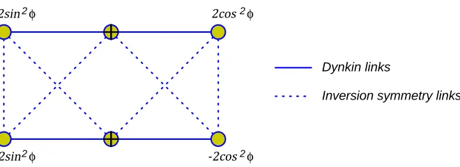
The integer mis the winding number of the string. The equations can be summarized in a diagram shown in fig. 1. The nodes of the diagram correspond to the densities ρ±
n. The
left hand side of the equations is determined by the Dynkin labels, and the right hand side by the links. The original Dynkin links from the Cartan matrix (7.18) determine coefficients in the first term in (7.17). The second term, which is associated with the inversion symmetry, produces additional links on the Dynkin diagram, shown in fig. 1 by broken lines.
18In this section, we denote quantities related to the left (right)d(2,1;α) by +(
−).
19In the AdS
5/CFT4 case,λ is also the ’t Hooft coupling of the dual super-Yang-Mills theory. The
precise nature of the parameterλin the CFT2dual of theAdS3×S3×S3×S1background is not clear
2 2
2 2
φ
φ
φ
φ
Dynkin links
[image:24.595.133.463.91.211.2]Inversion symmetry links
Figure 1: The Dynkin diagram of the classical Bethe equations.
The light-cone energy (E − J = (D−J)/√λ) and the worldsheet momentum of the solution are given by
P = −2X
s=±
s
sin2φ
Z
dx
x ρ
s
1(x) + cos2φ
Z
dx
x ρ
s
3(x)
(7.24)
E − J = 2X
s=±
sin2φ
Z
dx
x2 ρ
s
1(x) + cos2φ
Z
dx
x2 ρ
s
3(x)
. (7.25)
Physical states should in addition satisfy the level-matching condition P ∈2πZ.
7.3
BMN limit
The trivial solution of the finite-gap equations, with zero densities, describes the BMN vacuum. The BMN modes correspond to the vanishingly small cuts whose position is determined by the no-force condition, the vanishing of the left-hand side the Bethe equations. For instance, the left hand side of (7.21) vanishes at
1
xn
= J n sin
2φ
−
r
sin4φ+ n 2
J2
!
, (7.26)
where we have set the winding number m to zero and also neglected the difference between E, which enters the classical Bethe equations, and J, which plays the role of the length of the string in the light-cone gauge. This is justified for small deviations from the BMN vacuum. The set of points {xn} determines the locus at which short
cuts with infinitesimal filling fractions can emerge. The solution with infinitesimal cuts corresponds to exciting a number of BMN modes. Their occupation numbers Nn are
proportional to the filling fractions of the cuts:
Sn =
Z
C1,n
dxρ(x). (7.27)
The precise relationship between the occupation numbers are the filling fractions is de-rived in [12]:
Sn =
πNn
√
λ 1 +
s
1 + n2
J2sin4φ
!
The energy then is
E − J =X
n
2Snsin2φ
x2n = 2π
√
λ
X
n
Nn
r
sin4φ+ n 2
J2 −sin 2φ
!
,
Because the length of the string in the light-cone gauge is 2πJ, the combination n/J plays the role of the worldsheet momentum. The spectrum of small fluctuations thus describes particles with the dispersion relation
ε(p) =
q
p2+ sin4φ . (7.28)
Similarly, the densities ρ±3(x) describe particles with mass cos2φ. The heavy modes are more tricky. They correspond to stacks [60] that cross from node 1 to node 3 through node 2. The stack, roughly speaking, is a set of overlapping densities on different nodes. In this particular case it is a simultaneous solution of a pair of equations
2 sin2φJ x
x2−1 = 2πn,
2 cos2φJ x
x2 −1 = 2πm. (7.29)
The solution is only possible in the thermodynamic limit n ∼ m ∼ J → ∞, since n and m must satisfy n/m= tan2φ, in which case the stack corresponds to a particle of mass 1. The stacks are also responsible for the correct four-fold degeneracy at each mass level. For instance, the bosonic members of theP SU(1|1)×P SU(1|1) multiplet of mass sin2φare the single-node solutions for the densitiesρ+1 andρ−1. The fermions in the same multiplet are the 1+−2+ and 1−−2− stacks.
We have correctly reproduced the massive part of the BMN spectrum. However, the massless modes, that we also found in section 5, are completely missing. As we explain below in section 8, the finite-gap equations do not capture massless modes and describe only those solutions of the sigma-model in which the massless modes are not excited. Although this makes our analysis incomplete, we will proceed with quantization of the classical Bethe equations obtained above.
7.4
Quantum Bethe equations
Dynkin links
Fermionic inversion symmetry links
[image:26.595.127.457.92.204.2]BES/BHL phase
Figure 2: The Dynkin diagram of the asymptotic Bethe ansatz.
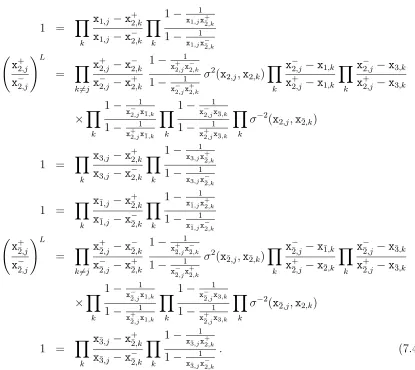
links of type appear in the equations); (iii) the inversions symmetry links that connect the momentum-carrying nodes pairwise. It is quite remarkable that the classical Bethe equations in our case also contain only these three types of structural elements. We can thus apply the same set of rules as in AdS5/CFT4 and AdS4/CFT3 to discretize the classical Bethe equations derived above. There is one subtlety though. The discretization is straightforward only when the elements of the Cartan matrix are integers, which is not the case for the d(2,1;α) algebra in general. The two exceptions areφ =π/4 (considered here) and φ= 0 (discussed below), and we will restrict our attention to these two special cases.
When φ = π/4, the d(2,1;α) superalgebra coincides with osp(4|2) whose Cartan matrix has integer entries. In quantum theory, the cuts of the classical spectral curve get discretized and become the arrays of Bethe roots. The asymptotic Bethe ansatz determines the positions of the roots in the spectral plane, xl,i, through a system of
discrete functional equations (the Bethe equations). The coupling constant of the sigma-model (playing the role of~) 2π/√λdoes not appear in the equations explicitly and only
enters through the quantum parameters x± defined by the Jukovsky map:
x±+ 1
x± =x+ 1
x ±
i
2h(λ). (7.30)
The function h(λ) cannot determined by integrability alone, but at strong coupling should behave as
h(λ)≈
√
λ
2π (λ→ ∞), (7.31)
in order to reproduce the correct dispersion relation ε(p) =p
p2+ 1/4.