Reduced-Rank STAP Schemes for Airborne Radar Based on Switched Joint Interpolation, Decimation and Filtering Algorithm

White Rose Research Online URL for this paper:

http://eprints.whiterose.ac.uk/30666/

Version: Submitted Version

Article:

Fa, R., de Lamare, R.C. and Wang, L. (2010) Reduced-Rank STAP Schemes for Airborne

Radar Based on Switched Joint Interpolation, Decimation and Filtering Algorithm. IEEE

Transactions on Signal Processing. 5447728. pp. 4182-4194. ISSN 1053-587X

https://doi.org/10.1109/TSP.2010.2048212

[email protected] https://eprints.whiterose.ac.uk/ Reuse

Items deposited in White Rose Research Online are protected by copyright, with all rights reserved unless indicated otherwise. They may be downloaded and/or printed for private study, or other acts as permitted by national copyright laws. The publisher or other rights holders may allow further reproduction and re-use of the full text version. This is indicated by the licence information on the White Rose Research Online record for the item.

Takedown

If you consider content in White Rose Research Online to be in breach of UK law, please notify us by

White Rose Research Online

[email protected]

Universities of Leeds, Sheffield and York

http://eprints.whiterose.ac.uk/

This is an author produced version of a paper published in

Chemical Communications

White Rose Research Online URL for this paper:

http://eprints.whiterose.ac.uk/30666

Published paper

Fa, R, de Lamare, R.C, Wang, L(2010)

Reduced-Rank STAP Schemes for Airborne Radar Based on Switched Joint

Interpolation, Decimation and Filtering Algorithm

IEEE TRANSACTIONS ON SIGNAL PROCESSING

58 (8) 4182-4194

For R

eview Only

Reduced-Rank STAP Schemes for Airborne Radar

Based on Switched Joint Interpolation, Decimation

and Filtering Algorithm

Rui Fa, Rodrigo C. de Lamare and Lei Wang

Abstract— In this paper, we propose a reduced-rank space-time adaptive processing (STAP) technique for airborne phased array radar applications. The proposed STAP method performs dimensionality reduction by using a reduced-rank switched joint interpolation, decimation and filtering algorithm (RR-SJIDF). In this scheme, a multiple-processing-branch (MPB) framework, which contains a set of jointly optimized interpolation, decima-tion and filtering units, is proposed to adaptively process the observations and suppress jammers and clutter. The output is switched to the branch with the best performance according to the minimum variance criterion. In order to design the decimation unit, we present an optimal decimation scheme and a low-complexity decimation scheme. We also develop two adaptive implementations for the proposed scheme, one based on a recursive least squares (RLS) algorithm and the other on a constrained conjugate gradient (CCG) algorithm. The proposed adaptive algorithms are tested with simulated radar data. The simulation results show that the proposed RR-SJIDF STAP schemes with both the RLS and the CCG algorithms converge at a very fast speed and provide a considerable SINR improvement over the state-of-the-art reduced-rank schemes.

Index Terms_{— Space-time adaptive processing (STAP),}

reduced-rank techniques, airborne phased array radar.

I. INTRODUCTION

S

PACE-time adaptive processing (STAP) techniques have been motivated as a key enabling technology for advanced airborne radar applications following the landmark publication by Brennan and Reed [1]. A great deal of attention has been given to STAP algorithms and much of the work has been done in the past three decades [2]–[15]. It is fully understood that STAP techniques can improve slow-moving target detection through better mainlobe clutter suppression, provide better detection in combined clutter and jamming environments, and offer a significant increase in output signal-to-interference-plus-noise-ratio (SINR). However, due to its large computational complexity cost by the matrix inversion operation, the optimum STAP processor is prohibitive for practical implementation. Furthermore, an even more challeng-ing issue is raised by full-rank STAP techniques when the number of elements M in the filter is large. It is well-known that K ≥ 2M independent and identically distributed (i.i.d) training samples are required for the filter to achieve the steady performance [16]. Thus, in dynamic scenarios the full-rank STAP with largeM usually fail or provide poor performance

This work is funded by the Ministry of Defence (MoD), UK. Project MoD, Contract No. RT/COM/S/021.The authors are with the Communications Research Group, Department of Electronics, University of York, YO10 5DD, United Kingdom. Email:{rf533, rcdl500, lw517}@ohm.york.ac.uk

in tracking target signals contaminated by interference and noise.

Reduced-rank adaptive signal processing has been consid-ered as a key technique for dealing with large systems in the last decade. The basic idea of the reduced-rank algorithms is to reduce the number of adaptive coefficients by project-ing the received vectors onto a lower dimensional subspace which consists of a set of basis vectors. The adaptation of the low-order filter within the lower dimensional subspace results in significant computational savings, faster convergence speed and better tracking performance. The first statistical reduced-rank method was based on a principal-components (PC) decomposition of the target-free covariance matrix [4]. Another class of eigen-decomposition methods was based on the cross-spectral metric (CSM) [8]. Both the PC and the CSM algorithms require a high computational cost due to the eigen-decomposition. A family of the Krylov subspace methods has been investigated thoroughly in the recent years. This class of reduced-rank algorithms, including the multistage Wiener filter (MSWF) [12], [18] and the auxiliary-vector filters (AVF) [19]–[21], projects the observation data onto a lower-dimensional Krylov subspace. These methods are very complex to implement in practice and suffer from numerical problems despite their improved convergence and tracking per-formance. The joint domain localized (JDL) approach, which is a beamspace reduced-dimension algorithm, was proposed by Wang and Cai [22] and investigated in both homogeneous and nonhomogeneous environments in [23], [24], respectively. Recently, reduced-rank adaptive processing algorithms based on joint iterative optimization of adaptive filters [25], [26] and based on an adaptive diversity-combined decimation and interpolation scheme [27], [28] were proposed, respectively. In our prior work [26], a joint iterative optimization of adaptive filters STAP scheme using the linearly constrained minimum variance (LCMV) was considered and applied to airborne radar applications, resulting in a significant improvement both in convergence speed and SINR performance as compared with the existing reduced-rank STAP algorithms.

The goal of this paper is to devise cost-effective STAP algo-rithms that have substantially faster convergence performance than existing methods. This enables the radar system with a significantly better probability of detection (PD) with limited

training. We develop a reduced-rank STAP design based on a switched joint interpolation, decimation and filtering (RR-SJIDF) algorithm for airborne radar systems. In this scheme, the number of elements for adaptive processing is substantially

For R

eview Only

reduced, resulting in considerable computational savings and

very fast convergence performance for radar applications. The proposed approach obtains the subspace of interest via a mul-tiple processing branch (MPB) framework which consists of a set of simple interpolation, decimation and filtering operations. Unlike the previous work in [27], multiple interpolators and reduced-rank filters are employed in the MPB framework and are designed with the LCMV criterion. For each branch, the interpolator and the reduced-rank filter can be jointly optimized by minimizing a cost function subject to linear con-straints. We describe an optimal decimation scheme and a low-complexity decimation scheme for the proposed structure. We also derive two adaptive implementations using the recursive least squares (RLS) and the constrained conjugate gradient (CCG) algorithms for the proposed scheme and evaluate their computational complexity. The numerical results show that the proposed RR-SJIDF STAP schemes with both the RLS and the CCG algorithms converge at a very fast speed and provide a considerable SINR improvement with significantly low complexity compared with the existing reduced-dimension and reduced-rank algorithms, namely, the JDL, the MSWF and the AVF algorithms.

The main contributions of our paper are listed as follows: i) A reduced-rank STAP scheme based on SJIDF algorithm

for airborne radar platform is proposed.

ii) In the proposed scheme, a MPB framework is introduced. For each branch, the interpolator and reduced-rank fil-ters are jointly optimized by minimizing the modified minimum variance (MV) cost function with a set of constraints.

iii) Two efficient adaptive implementations using the RLS and the CCG algorithms are developed for the proposed STAP scheme and a detailed study of their computational complexity requirements is provided.

iv) Algorithms for automatically adjusting the rank of the proposed SJIDF scheme are developed.

v) A study and comparative analysis of reduced-rank STAP techniques for radar systems is carried out.

This paper is organized as follows. Section II states the signal model, the optimum full-rank STAP algorithm and the fundamentals of reduced-rank signal processing. Section III presents the proposed reduced-rank STAP scheme, describes the proposed joint iterative optimization of the interpolation, decimation and filtering tasks, and details the proposed dec-imation schemes. In Section IV, we develop two adaptive implementations using the RLS and the CCG algorithms and algorithms for automatically adjusting the rank of the proposed scheme. In Section V, we discuss the convergence properties of the optimization of the proposed scheme. The performance assessment of the proposed reduced-rank STAP scheme is provided in Section VI using simulated radar data. Finally, conclusions are given in Section VII.

II. SIGNALMODEL, RADARSIGNALPROCESSING AND

PROBLEMSTATEMENT

The system under consideration is a pulsed Doppler radar residing on an airborne platform. The radar antenna is a uni-formly spaced linear array antenna consisting ofN elements.

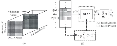
H0: Target Absent H1: Target Present

(a)

KRa

nge G ates

PRI,JPulses

A

nt

enna

,

N

E

le

m

ent

s

i-th Range Gates

r(i-1)

r(i+1)

r(i)

å

=

=

K i

H

i i K 1

) ( ) ( 1

ˆ _{r r}

R STAP

r(i) d(i)

h

H1

H0 H1 < > H0

[image:4.612.323.554.50.141.2]

(b)

Fig. 1. (a) The Radar CPI datacube. (b) The STAP schematic.

Radar returns are collected in a coherent processing interval (CPI), which is referred to as the 3-D radar datacube shown in Fig. 1(a), where K denotes the number of samples collected to cover the range interval. The data is then processed at one range of interest, which corresponds to a slice of the CPI datacube. This slice is a J ×N matrix which consists of N×1spatial snapshots forJ pulses at the range of interest. It is convenient to stack the matrix column-wise to form the M×1, M=JN vectorr(i), termed thei-th range gate space-time snapshot,1≤i≤K [1].

A. Signal Model

The objective of a radar is to ascertain whether targets are present in the data. Thus, given a space-time snapshot, radar detection is a binary hypothesis problem, where hypothesisH0 corresponds to target absence and hypothesisH1corresponds to target presence. The radar space-time snapshot is then expressed for each of the two hypotheses in the following form,

H0:r(i) =v(i), H1:r(i) =as+v(i),

(1)

where a is a zero-mean complex Gaussian random variable with variance σ2

s, v(i) denotes the input

interference-plus-noise vector which consists of clutterrc(i), jammingrj(i)and

the white noisern(i). These three components are assumed to

be mutually uncorrelated. Thus, theM×Mcovariance matrix Rof the undesired clutter-plus-jammer-plus-noise component can be modelled as

R=E{v(i)vH(i)}=Rc+Rj+Rn, (2)

where H represents Hermitian transpose and E denotes ex-pectation. According to [6], the noise covariance noise matrix Rn = E{rn(i)rHn(i)} can be written as a scaled identity

matrixσ2

nIM, whereσ2nis the noise power. The clutter signal

can be modeled as the superposition of a large number of independent clutter patches with evenly distributed in azimuth about the receiver. Thus, the clutter covariance matrix can be expressed as

Rc=E{rc(i)rHc (i)}

=

Nr

X

k=1

Nc

X

l=1 ξc

kl

£

b(ϑc

kl)b(ϑckl)H

¤

⊗£a(̟c

kl)a(̟ckl)H

¤

,

(3)

where Nr denotes the number of range ambiguities and Nc

denotes the number of the clutter patches. ξc

kl is the power

For R

eview Only

of reflected signal by the kl-th clutter patch. The notation⊗

denotes Kronecker product. b(ϑc

kl) and a(̟ckl), respectively,

denote the spatial steering vector with the spatial frequency ϑc

kl and the temporal steering vector with the normalized

Doppler frequency̟c

kl for thekl-th clutter patch, which can

be expressed as follows

b(ϑ) = 

     

1

e−j2πϑ

e−j2π2ϑ

.. . e−j2π(N−1)ϑ



     

, a(̟) = 

     

1

e−j2π̟

e−j2π2̟

.. . e−j2π(K−1)̟



     

, (4)

where ϑ = d

λcos(φ) sin(θ) and ̟ = fd/fr, where λ is

wavelength; d is interelement spacing which is normally set to half wavelength; φ and θ are elevation and azimuth, respectively; fd and fr are Doppler frequency and pulse

repetition frequency, respectively. The jamming covariance matrixRj=E{rj(i)rHj (i)}can be written as

Nj

X

q=1 ξj

q

£

b(ϑj q)b(ϑjq)H

¤ ⊗IK,

where ξj

q is the power of the q-th jammer. b(ϑjq) is the

spatial steering vector with the spatial frequency ϑj q of the

q-th jammer andNj is the number of jammers. The vectors,

which is theM×1normalized space-time steering vector in the space-time look-direction, can be defined as:

s=pξtb(ϑt)⊗a(̟t), (5)

wherea(̟t)is theK×1normalized temporal steering vector

at the target Doppler frequency ̟t and b(ϑt) is the N ×1

normalized spatial steering vector in the direction provided by the target spatial frequencyϑtandξtdenotes the power of the

target.

B. Optimum Radar Signal Processing

To detect the presence of targets, each range bin is processed by an adaptive 2D beamformer (to achieve maximum output SINR) followed by a hypothesis test to determine the target presence or absence. Here, we assume that the secondary data

{r(i)}K

i=1 are i.i.d training samples. The optimum full-rank STAP [1] obtained by an unconstrained optimization of the SINR is given as follows:

ωopt=kR−1s, (6)

where kis an arbitrary nonzero complex number. By solving the LCMV problem as [37]

ωopt= arg min

ω(i)

ωH(i)Rω(i) s. t. sHω(i) = 1, (7) the optimal constrained weight vector for maximizing the output SINR, while maintaining a normalized response in the target spatial-Doppler look-direction was originally given in [29] by

ωopt=

R−1s

sH_R−1_s. (8) The solution in (8) is also known as the minimum variance distortionless response (MVDR) solution.

C. Reduced-Rank Signal Processing

The basic idea of reduced-rank algorithms is to reduce the number of adaptive coefficients by projecting the received vectors onto a lower dimensional subspace as illuminated in the figure. Let SD denote theM×Dprojection matrix with

column vectors which are anM×1basis for aD-dimensional subspace, where D < M. Thus, the received signal r(i) is transformed into its reduced-rank version¯r(i) given by

¯

r(i) =SHDr(i). (9)

The rank signal is processed by an adaptive reduced-rank filter ω¯(i)∈ CD×1_{. Subsequently, the decision is made} based on the filter output y(i) = ¯ωH_{(i)¯r(i). By solving the}

optimization problem as below

¯

ωopt= arg min

¯ ω(i)

¯

ωH(i) ¯Rω¯(i), subject to ω¯H(i)¯s= 1, (10) the optimum MVDR solution for the reduced-rank weight vectorω¯optis obtained [26]

¯

ωopt=

¯

R−1¯s

¯

sH_R¯−1_¯s, (11) where R¯ = SH

DRSD denotes the reduced-rank covariance

matrix and¯s=SH

Dsdenotes the reduced-rank steering vector.

The challenge left to us is how to efficiently design and optimize the projection matrixSD. The PC method which is

also known as the eigencanceller method [4] suggested to form the projection matrix using the eigenvectors of the covariance matrix R corresponding to the eigenvalues with significant magnitude. The CSM method, a counterpart of the PC method belonging to the eigen-decomposition algorithm family, out-performs the PC method because it employs the projection matrix which contains the eigenvectors which contribute the most towards maximizing the SINR [17]. A family of closely related reduced-rank adaptive filters, such as the MSWF [18] and the AVF [19], employs a set of basis vectors as the projection matrix which spans the same subspace, known as the Krylov subspace. The Krylov subspace is generated by taking the powers of the covariance matrix of observations on a cross-correlation (or steering) vector. Despite the improved convergence and tracking performance achieved with these methods, the remaining problems are their high complexity and the existence of numerical problems for implementa-tion. The joint domain localized (JDL) approach, which is a beamspace reduced-dimension algorithm, was proposed by Wang and Cai [22] and investigated in both homogeneous and nonhomogeneous environments in [23], [24], respectively. Recently, reduced-rank filtering algorithms based on joint iterative optimization of adaptive filters [25], [26] and based on an adaptive diversity-combined decimation and interpolation scheme [27], [28] were proposed, respectively.

III. PROPOSEDRR-SJIDF SCHEME

In this section, we detail the proposed adaptive reduced-rank filtering scheme based on the switched joint interpo-lation, decimation and filtering (RR-SJIDF). The reduced-rank adaptive filtering scheme based on combined decimation

For R

eview Only

T1 T2 TB Adaptive Algorithm ) ( ) ( )

(i i i

y b H b r ù = ) ( 1i r ) ( 1 , i I r ) (i r ) ( 1i ù ) ( 2i ù ) (i B ù ) ( 2i r ) (i B r vB(i)

v₁(i)

v₂(i) rI,2(i)

) (

,Bi I

r

(i)

D,1 S (i) B D, S (i)

[image:6.612.76.302.49.178.2]

D,2 S

Fig. 2. Proposed Adaptive Reduced-Rank Filtering Scheme (RR-SJIDF).

and interpolation filtering was presented in [27], [28]. In this work, we develop a reduced-rank STAP algorithm based on the SJIDF scheme for airborne radar applications, whose schematic is shown in Fig. 2. The motivation for designing a projection matrix based on interpolation and decimation comes from two observations. The first is that rank reduction can be performed by constructing new samples with interpolators and eliminating (decimating) samples that are not useful in the STAP design. The second comes from the structure of the projection matrix, whose columns are a set of vectors formed by the interpolators and the decimators.

A. Overview of the RR-SJIDF Scheme

Here, we explain how the proposed RR-SJIDF scheme works and its main building blocks. In this scheme, the number of elements for adaptive processing is substantially reduced, resulting in considerable computational savings and very fast convergence performance for the radar applications. The pro-posed approach obtains the subspace of interest via a multiple processing branch (MPB) framework. The M ×1 received vector r(i) = [r0(i), r1(i),· · ·, rM−1(i)]T is processed by a MPB framework withBbranches, where each spatio-temporal processing branch contains an interpolator filter, a decimation unit and a reduced-rank filter. In the b-th branchb ∈ [1, B], the received vector r(i) is filtered by the interpolator filter

¯

υb(i) = [υ0,b(i), υ1,b(i),· · ·, υI−1,b(i)]T with filter length

I, yielding the interpolated received vector r′

b(i) with M

samples, which is expressed by

r′b(i) =Vb(i)r(i), (12)

where theM×MToeplitz convolution matrixVb(i)is given

by

Vb(i) =

             

υ0,b(i) 0 . . . 0

..

. υ0,b(i) . . . 0

υI−1,b(i) ... . . . 0

0 υI−1,b(i) . . . 0

0 0 . .. 0

..

. ... . .. ...

0 0 . . . υ0,b(i)

              . (13)

In order to facilitate the description of the scheme, let us express the vector r′_b(i) in an alternative way which will be useful in the following through the equivalence:

r′b(i) =Vb(i)r(i) =R0(i)¯υb(i), (14)

where the M×I matrixR_{0(i)with the samples ofr(i) has}

a Hankel structure [30] and is described by

R_{0(i) =}

              

r0(i) r1(i) . . . rI−1(i) r1(i) r2(i) . . . rI(i)

..

. ... . . . ... rM−I(i) rM−I+1(i) . . . rM−1(i) rM−I+1(i) rM−I+2(i) . .. 0

..

. ... . .. ... rM−2(i) rM−1(i) 0 0 rM−1(i) 0 0 0

               . (15)

The dimensionality reduction is performed by a decimation unit with D×M decimation matrices Tb that projectsrI(i)

ontoD×1vectors¯rb(i)withb= 1, . . . , B, whereD=M/L

is the rank andLis the decimation factor. TheD×1vector

¯

rb(i)for branchbis expressed by

¯

rb(i) =TbVb(i)

| {z }

SD,b(i)

r(i) =Tbr′b(i) =TbR0(i)¯υb(i), (16)

where SD,b(i) is the equivalent projection matrix and the

vector ¯rb(i) for branch b is used in the minimization of the

output power for branchb, which is given by

|yb(i)|2=|ω¯Hb (i)¯rb(i)|2.

The output at the end of the MPB framework y(i)is selected according to:

y(i) =ybs(i) when bs= arg min

1≤b≤B|yb(i)|

2_{, (17)}

where Bis a parameter to be set by the designer.Essential to the derivation of the joint iterative optimization that follows is to express the output of the RR-SJIDF STAP yb(i) =

¯

ωH

b (i)¯rb(i) as a function ofυ¯b(i), the decimation matrixTb

and ω¯H

b (i) as follows:

yb(i) = ¯ωHb (i)SD,b(i)r(i)

= ¯ωHb (i)TbR0(i)¯υb(i) = ¯ωHb (i)¯rω,b¯ (i)

= [¯υH_b (i)RH

0(i)THb ω¯b(i)]∗= [¯υHb (i)¯rυ,b¯ (i)]∗. (18)

where ¯r¯ω,b(i) = TbR0(i)¯υb(i) denotes the reduced-rank

signal with respect to ω¯b(i) and ¯r¯υ,b(i) =RH0(i)THb ω¯b(i)

denotes the reduced-rank signal with respect to υ¯b(i), (·)∗

denotes the conjugate operation. The expression (18) indicates that the dimensionality reduction carried out by the proposed scheme depends on finding appropriate υ¯b(i), ω¯b(i) and

Tb. In the following subsections we will derive the joint

optimizations of υ¯b(i) and ω¯b(i) and design the decimation

unitTb.

For R

eview Only

B. Optimization of the Filters

In this part, we describe the proposed joint and iterative optimization algorithm that adjusts the parameters of the interpolator filterυ¯b(i)and the reduced-rank filterω¯b(i)with

the given decimation pattern Tb. According to the LCMV

criterion, the optimization problem is given by

minE

h¯ ¯

¯ω¯Hb(i)TbR0(i)¯υb(i)

¯ ¯ ¯

2i

subject toω¯Hb (i)TbS0υ¯b(i) = 1, b= [1,· · ·, B],

(19)

where S_{0is M×I steering matrix with a Hankel structure,}

which has the same form asR_0(i)

S₀₌



             

s0 s1 . . . sI−1 s1 s2 . . . sI

..

. ... . . . ... sM−I sM−I+1 . . . sM−1 sM−I+1 sM−I+2 . .. 0

..

. ... . .. ... sM−2 sM−1 0 0

sM−1 0 0 0



             

. (20)

The constrained cost function in (19) can be transformed into unconstrained one by introducing a Lagrangian multiplier, which is given as

L( ¯ωb(i),υ¯b(i)) =E

h¯

¯ω¯Hb (i)TbR0(i)¯υb(i)

¯ ¯2

i

+ 2ℜ©λ£ω¯Hb(i)TbS0υ¯b(i)−1

¤ª

, (21)

whereλis the Lagrangian multiplier. By fixingω¯(i)andυ¯(i), respectively, (21) can be rewritten into two equations as

L(¯υb(i)) =E

h¯ ¯υ¯H

b (i)¯rυ,b¯ (i)

¯ ¯2

i

+ 2ℜ©λυ,b¯

£ ¯

υH

b (i)¯sυ,b¯ (i)−1

¤ª

,

L( ¯ωb(i)) =E

h¯

¯ω¯Hb (i)¯rω,b¯ (i)

¯ ¯2

i

+ 2ℜ©λω,b¯

£ ¯

ωHb(i)¯sω,b¯ (i)−1

¤ª

,

where ¯sυ,b¯ (i) = THb (i)S H

0ω¯b(i) and ¯sω,b¯ (i) = TbS0υ¯b(i)

denote the reduced-rank steering vectors with respect toυ¯(i)

and ω¯(i), respectively. λυ,b¯ and λω,b¯ are the Lagrangian multipliers for υ¯(i) and ω¯(i), respectively. By minimizing

L(¯υb(i))and solving forλυ,b¯ , we get

¯

υb(i) =

¯

R−_¯υ,b1¯s¯υ,b(i)

¯sH

¯

υ,b(i) ¯R

−1

¯

υ,b¯sυ,b¯ (i)

, (22)

whereR¯υ,b¯ =E

h

¯rυ,b¯ (i)¯rHυ,b¯ (i)

i

. By minimizingL( ¯ωb(i))and

solving forλω,b¯ , we get

¯

ωb(i) =

¯

R−_ω,b¯1¯sω,b¯ (i)

¯

sH

¯

ω,b(i) ¯R

−1

¯

ω,b¯s¯ω,b(i)

, (23)

where R¯ω,b¯ =E

h

¯rω,b¯ (i)¯rHω,b_¯ (i)

i

. Note that the joint iterative optimization of the interpolation filters {υ¯b(i)|b= 1, ..., B}

and the reduced-rank filters {ω¯b(i)|b= 1, ..., B} are

per-formed separately in all the processing branches.

C. Design of the Decimation Unit

Here, we consider two strategies for the design of the decimation unit Tb(i). We constrain the design of Tb(i) so

that the elements of the matrix only take the value 0 or 1. This corresponds to the decimation unit simply keeping or discarding the samples. The first strategy exhaustively explores all possible decimation patterns which select D samples out ofM samples, this is therefore the optimal approach. In this case, the scheme can be viewed as a combinatorial problem and the total number of patterns B, equal to

B=M·(M−1)· · ·(M−D+ 1) = µ

M D

¶

. (24)

However, the optimal decimation scheme described above is too complex for practical use since it needs Dpermutations of M samples for each snapshot and carries out an exhaustive search over all possible patterns. Therefore, an alternative decimation scheme with low-complexity that renders itself to practical use is of great interest. To this end, we consider the second decimation scheme which we call pre-stored deci-mation unit (PSDU). The PSDU scheme employs a structure formed in the following way

Tb= [φb,1 φb,2 ... φb,D], (25)

where the M ×1 vector φ_b,d denotes the dth basis vector of the bth decimation unit, d = 1, ..., D, b = 1, ..., B, and is composed of a single 1and (M−1) 0s, according to the following

φb,d= [0, ... , 0

| {z }

zb,d

, 1, 0, ... , 0

| {z }

M−zb,d−1

], (26)

where zb,d is the number of zeros before the only element

equal to one. We set the value ofzb,d in a deterministic way

which can be expressed as

zb,d=

M

D ×(d−1) + (b−1). (27)

It should be remarked that other designs have been investigated and this structure has been adopted due to an excellent trade-off between performance and complexity.

IV. ADAPTIVEALGORITHMS

Adaptive implementations of the LCMV beamformer were subsequently reported with the RLS and the CG algorithms [16], [31]–[33]. Here, we develop the RLS and the CCG algorithms that adjust the parameters of the interpolation filters and the reduced-rank filters for the MPB structure based on the minimization of the CMV cost function. Furthermore, we compare the complexity of the proposed RR-SJIDF algorithms with other existing algorithms, namely, the full-rank RLS filter, the JDL, the MSWF and the AVF algorithms, in terms of multiplications and additions per snapshot.

For R

eview Only

A. Recursive Least Squares (RLS) algorithm

Here, we describe an RLS algorithm that adaptively adjusts the coefficients of the interpolation filters{υ¯b(i)|b= 1, ..., B}

and the reduced-rank filters{ω¯b(i)|b= 1, ..., B}based on the

least squares (LS) cost functions, which are shown as below:

LLS(¯υb(i)) = i

X

n=1 αi−n¯

¯υ¯Hb(n)¯rυ,b¯ (n)

¯ ¯2

+ 2ℜ©λυ,b¯

£ ¯

υHb (i)¯sυ,b¯ (i)−1

¤ª

,

LLS( ¯ωb(i)) = i

X

n=1

αi−n¯¯ω¯_bH(n)¯rω,b¯ (n)

¯ ¯2

+ 2ℜ©λω,b¯

£ ¯

ωHb (i)¯sω,b¯ (i)−1

¤ª

, (28)

where αis the forgetting factor. By computing the gradients of LLS(¯υb(i)) and LLS( ¯ωb(i)), and equating them to zero

and solving forλυ,b¯ andλω,b¯ , respectively, we obtain

¯

υb(i) =

ˆ¯

R−_υ,b¯1(i)¯sυ,b¯ (i)

¯

sH

¯

υ,b(i) ˆ¯R

−1

¯

υ,b(i)¯sυ,b¯ (i)

,

¯

ωb(i) =

ˆ¯

R−_¯ω,b1(i)¯sω,b¯ (i)

¯

sH

¯

ω,b(i) ˆ¯R

−1

¯

ω,b(i)¯sω,b¯ (i)

,

(29)

where Rˆ¯υ,b¯ (i) =

Pi

n=1αi−n¯rυ,b¯ (n)¯rυ,bH¯ (n) and Rˆ¯ω,b¯ (i) =

Pi

n=1αi−n¯r¯ω,b(n)¯rHω,b_¯ (n) denote the time averaged

correla-tion matrices with respect toω¯b(i)andυ¯b(i), respectively. By

employing the matrix inversion lemma, and definingPυ,b¯ (i) =

ˆ¯

R−_υ,b¯1(i) and Pω,b¯ (i) = ˆ¯R−ω,b_¯1(i),respectively, and the gain

vectors ¯kυ,b¯ (i) and ¯kω,b¯ (i) are expressed, respectively, as follows

¯

kυ,b¯ (i) =

P¯υ,b(i−1)¯rυ,b¯ (i) α+ ¯rH

¯

υ,b(i)Pυ,b¯ (i−1)¯rυ,b¯ (i) ,

¯

kω,b¯ (i) =

Pω,b¯ (i−1)¯rω,b¯ (i) α+ ¯rH

¯

ω,b(i)Pω,b¯ (i−1)¯rω,b¯ (i) ,

(30)

and thus we can rewritePυ,b¯ (i)and Pω,b¯ (i) recursively as Pυ,b¯ (i) =α−1P¯υ,b(i−1)−α−1k¯υ,b¯ (i)¯rHυ,b¯ (i)Pυ,b¯ (i−1), Pω,b¯ (i) =α−1Pω,b¯ (i−1)−α−1k¯ω,b¯ (i)¯rHω,b¯ (i)Pω,b¯ (i−1),

(31)

wherePυ,b¯ (0)andPω,b¯ (0)are initialized toδ−1I, whereδis a small positive constant andIis the identity matrix. It is worth remarking that ¯rH

¯

ω,b(i),¯rHυ,b¯ (i),¯sω,bH¯ (i) and ¯sHυ,b¯ (i) have to be updated as soon asυ¯b(i)andω¯b(i)are updated since they are

dependent onω¯b(i)andυ¯b(i), respectively. The output at the

end of the MPB frameworky(i)is selected according to:

y(i) =ybs(i) when bs= arg min

1≤b≤B|yb(i)|

2_{, (32)}

where

yb(i) = ¯ωHb (i)TbR0(i)¯υb(i). (33)

The algorithm is summaried in Table I.

TABLE I

THESJIDF SCHEMEUSING THERLSALGORITHM

Initialisation: for each branchb= 1,· · ·, B Pυ,b¯ (0) =δ−1IandP¯ω,b(0) =δ−1I,

¯

ωb(0) = [1,0,· · ·,0]T andυ¯b(0) = [1,0,· · ·,0]T, ¯

sυ,b¯ (1) =THbSH0ω¯b(0), ¯

sω,b¯ (1) =TbS0υ¯b(0),

Recursion: for each branchb= 1,· · ·, B

and each time instanti= 1,· · ·, K

STEP 1: updatingυ¯b(i)

¯

r¯υ,b(i) =THbRH0ω¯b(i−1), ¯

kυ,b¯ (i) =

P_¯υ,b(i−1)¯r_¯υ,b(i)

α+¯rH

¯

υ,b(i)Pυ,b¯ (i−1)¯rυ,b¯ (i)

,

Pυ,b¯ (i) =α−1Pυ,b¯ (i−1)−α−1k¯υ,b¯ (i)¯rHυ,b¯ (i)P¯υ,b(i−1), ¯

υb(i) =

P_¯υ,b(i)¯sυ,b(_¯ i) ¯

sH

¯

υ,b(i)Pυ,b¯ (i)¯s¯υ,b(i)

,

¯

sω,b¯ (i) =TbS0υ¯b(i), STEP 2: updatingω¯b(i)

¯

rω,b¯ (i) =TbR0υ¯b(i), ¯

kω,b¯ (i) =

Pω,b(_¯ i−1)¯rω,b(_¯ i)

α+¯rH

¯

ω,b(i)Pω,b¯ (i−1)¯r¯ω,b(i)

,

Pω,b¯ (i) =α−1Pω,b¯ (i−1)−α−1¯kω,b¯ (i)¯rHω,b¯ (i)P¯ω,b(i−1), ¯

ωb(i) =

Pω,b(_¯ i)¯sω,b(_¯ i) ¯

sω,b(_¯ i)HPω,b(_¯ i)¯sω,b(_¯ i),

¯

sυ,b¯ (i+ 1) =THbS H

0ω¯b(i),

STEP 3: Calculating the output ofb-th branch

yb(i) = ¯ωHb(i)TbR0(i)¯υb(i), Output:

y(i) =ybs(i) when bs= arg min1≤b≤B|yb(i)| 2_.

B. Constrained Conjugate Gradient (CCG) Algorithm

In this subsection, we develop a CCG algorithm to imple-ment the proposed RR-SJIDF STAP. According to (22) and (23) which were derived in the previous section based on CMV criterion, let us define two intermediate vectors, CG-based weight vectors,υ¯˜b(i) = ¯Rυ,b−_¯1¯sυ,b¯ (i)andω˜¯b(i) = ¯R−ω,b_¯1¯sω,b¯ (i), respectively, to solve the equations and save the computations. Thus, we may obtain υ¯b(i) = ˜υ¯b(i)/(¯sHυ,b¯ (i)˜υ¯b(i)) and

¯

ωb(i) = ˜ω¯b(i)/(¯sHω,b_¯ (i)˜ω¯b(i)). The solutions toR¯υ,b¯ υ˜¯b(i) =

¯

sυ,b¯ (i) and R¯ω,b¯ ω˜¯b(i) = ¯sω,b¯ (i), υ˜¯b(i) and ω˜¯b(i),

respec-tively, are given by solving two optimization problems as follows [33]–[35]

Φ(˜¯υb) = ˜υ¯Hb(i) ¯Rυ,b¯ ˜¯υb(i) + 2ℜ

© ¯

sHυ,b_¯ (i)˜υ¯b(i)

ª

,

˜ ¯

υb(i) = arg min

˜ ¯ υb(i)∈CI×1

Φ(˜¯υb), (34)

and

Φ(˜ω¯b) = ˜ω¯Hb(i) ¯Rω,b¯ ω˜¯b(i) + 2ℜ

©

¯sH_ω,b¯ (i)˜ω¯b(i)

ª

,

˜¯

ωb(i) = arg min

˜ ¯

υb(i)∈CD×1

Φ(˜ω¯b), (35)

where Φ(˜¯υb) and Φ(˜ω¯b) are cost functions with respect to

˜¯

υb(i) and ω˜¯b(i), respectively. The correlation matrices R¯υ,b¯ and R¯ω,b¯ , respectively, are estimated by

ˆ ¯

R¯υ,b(i) =λfRˆ¯υ,b¯ (i) + ¯r¯υ,b(i)¯rH¯υ,b(i),

ˆ ¯

Rω,b¯ (i) =λfRˆ¯ω,b¯ (i) + ¯rω,b¯ (i)¯rHω,b¯ (i),

(36)

For R

eview Only

where λf is the forgetting factor. Let us define gυ,b¯ (i) and

gω,b¯ (i) as residual vectors which are expressed, respectively, as follows

gυ,b¯ (i) =−▽υ˜¯bΦ(˜¯υb)

= ¯sυ,b¯ (i)−Rˆ¯υ,b¯ (i)˜¯υb(i),

(37)

and

gω,b¯ (i) =−▽ω˜¯bΦ(˜¯ωb)

= ¯sω,b¯ (i)−Rˆ¯ω,b¯ (i)˜¯ωb(i).

(38)

Thus, the CG-based weight vectors υ˜¯b(i) and ω˜¯b can be

recursively written as [36]

˜ ¯

υb(i) = ˜υ¯b(i−1) +αυ,b¯ (i)pυ,b¯ (i),

˜ ¯

ωb(i) = ˜ω¯b(i−1) +αω,b¯ (i)p¯ω,b(i),

(39)

where αυ,b¯ (i) and αω,b¯ (i) denote the step sizes. pυ,b¯ (i) and pω,b¯ (i) denote the direction vectors. According to [36], αυ,b¯ (i),α¯ω,b(i),p¯υ,b(i)andpω,b¯ (i)can, respectively, be given by

αυ,b¯ (i) =

n

λf

£

pHυ,b_¯ (i)gυ,b¯ (i−1)−pHυ,b¯ (i)¯sυ,b¯ (i)

¤

−ηυ¯pHυ,b¯ (i)gυ,b¯ (i−1)

o h

pH_υ,b¯ (i) ˆ¯Rυ,b¯ (i)pυ,b¯ (i)

i−1 ,

αω,b¯ (i) =

n

λf

£

pHω,b_¯ (i)gω,b¯ (i−1)−pHω,b¯ (i)¯sω,b¯ (i)

¤

−ηω¯pHω,b¯ (i)gω,b¯ (i−1)

o h

pH_ω,b¯ (i) ˆ¯Rω,b¯ (i)pω,b¯ (i)

i−1 ,

pυ,b¯ (i) =gυ,b¯ (i−1) +βυ,b¯ (i)pυ,b¯ (i), pω,b¯ (i) =gω,b¯ (i−1) +βω,b¯ (i)pω,b¯ (i),

(40)

where0≤ηυ¯, ηω¯≤0.5,βυ,b¯ (i)andβω,b¯ (i)can be computed as

β¯υ,b(i) =

gH

¯

υ,b(i) [gυ,b¯ (i) +λfs¯¯υ,b(i)−gυ,b¯ (i−1)] gH

¯

υ,b(i−1)g¯υ,b(i−1)

,

βω,b¯ (i) = gH

¯

ω,b(i) [gω,b¯ (i) +λfs¯ω,b¯ (i)−gω,b¯ (i−1)] gH

¯

ω,b(i−1)gω,b¯ (i−1)

. (41)

Thus, the interpolation filters υ¯b(i) and the reduced-rank

filters ω¯b(i) can be written as υ¯b(i) = ˜¯υb(i)/(¯sHυ,b_¯ (i)˜¯υb(i))

and ω¯b(i) = ˜¯ωb(i)/(¯sHω,b¯ (i)˜¯ωb(i)) based on the CG-based

weight vectors, respectively. The adaptive implementation of the proposed RR-SJIDF STAP using the CCG algorithm is summarised in Table II

C. Branch and Rank Selection

The performance of the algorithms described in the previous subsections highly depends on the parameters including the ranksD,I and the number of branchesB. In this subsection, we discuss the parameter settings to meet the best trade-off between the performance and the complexity. We have mentioned that in the previous section that the optimal number of branches is in (24), which is quite large. Within such range, we can claim that more branches, better performance for the proposed algorithm. However, considering the affordable complexity, we have to configure the algorithm with the

TABLE II

THESJIDF SCHEMEUSING THECCGALGORITHM

Initialisation: for each branchb= 1,· · ·, B ˜

¯

ωb(0) = [1,0,· · ·,0]T andυ¯˜b(0) = [1,0,· · ·,0]T, ¯

sυ,b¯ (1) =THbSH0ω¯b(0)and¯sω,b¯ (1) =TbS0υ¯b(0), gυ,b¯ (0) = ¯sυ,b¯ (1)andpυ,b¯ (1) =g¯υ,b(0),

gω,b¯ (0) = ¯sω,b¯ (1)andpω,b¯ (1) =gω,b¯ (0),

ˆ

Rυ,b¯ (0) =δ−1IandRˆω,b¯ (0) =δ−1I,

¯

υb(0) = ˜¯υb(0)/(¯sHυ,b¯ (1)˜υ¯b(0)), ¯

ωb(0) = ˜¯ωb(0)/(¯sHω,b¯ (1)˜ω¯b(0)), Recursion: for each branchb= 1,· · ·, B

and each time instanti= 1,· · ·, K

STEP 1: updatingυ¯b(i)

¯

r¯υ,b(i) =THbRH0ω¯b(i−1), ˆ

¯

Rυ,b¯ (i) =λfRˆ¯υ,b¯ (i) + ¯r¯υ,b(i)¯rHυ,b¯ (i),

α¯υ,b(i) =

n

λf

h

pH

¯

υ,b(i)gυ,b¯ (i−1)−pυ,bH¯ (i)¯s¯υ,b(i)

i

−η¯υpHυ,b¯ (i)gυ,b¯ (i−1)

o h

p_υ,bH_¯ (i) ˆR¯υ,b¯ (i)pυ,b¯ (i)

i−1

,

gυ,b¯ (i) =λfgυ,b¯ (i−1)−αυ,b¯ (i) ˆR¯¯υ,b(i)pυ,b¯ (i),

˜ ¯

υb(i) = ˜¯υb(i−1) +αυ,b¯ (i)pυ,b¯ (i),

β¯υ,b(i) =

gH_υ,b¯ (i)[gυ,b_¯ (i)+λf¯s¯υ,b(i)−g¯υ,b(i−1)] gH

¯

υ,b(i−1)g¯υ,b(i−1)

,

p¯υ,b(i) =gυ,b¯ (i−1) +βυ,b¯ (i)pυ,b¯ (i),

¯

υb(i) = ˜¯υb(i)/(¯sHυ,b¯ (i)˜υ¯b(i)), ¯

sω,b¯ (i) =TbS0υ¯b(i), STEP 2: updatingω¯b(i)

¯

rω,b¯ (i) =TbR0υ¯b(i), ˆ

¯

Rω,b¯ (i) =λfRˆ¯ω,b¯ (i) + ¯rω,b¯ (i)¯rHω,b¯ (i)

αω,b¯ (i) =

n

λf

h

pH

¯

ω,b(i)gω,b¯ (i−1)−pω,bH¯ (i)¯sω,b¯ (i)

i

−η¯ωpHω,b¯ (i)g¯ω,b(i−1)

o h

pH

¯

ω,b(i) ˆR¯ω,b¯ (i)p¯ω,b(i)

i−1

,

gω,b¯ (i) =λfgω,b¯ (i−1)−αω,b¯ (i) ˆR¯ω,b¯ (i)pω,b¯ (i),

˜ ¯

ωb(i) = ˜ω¯b(i−1) +αω,b¯ (i)p¯ω,b(i),

βω,b¯ (i) =

gHω,b_¯ (i)[gω,b(¯ i)+λf¯s¯ω,b(i)−gω,b(¯ i−1)] gH

¯

ω,b(i−1)gω,b(¯ i−1) , p¯ω,b(i) =gω,b¯ (i−1) +βω,b¯ (i)pω,b¯ (i),

¯

ωb(i) = ˜ω¯b(i)/(¯sHω,b¯ (i)˜ω¯b(i)), ¯

sυ,b¯ (i+ 1) =THbSH0ω¯b(i),

STEP 3: Calculating the output ofb-th branch

yb(i) = ¯ωHb(i)TbR0(i)¯υb(i), Output:

y(i) =ybs(i) when bs= arg min1≤b≤B|yb(i)|2.

number of branches as small as possible and meanwhile achieving competitive performance. As will be shown in the simulation results, the proposed algorithms with the number of branches Bequal to 4 or 5 have good trade-offs between the performance and the complexity. Since the performance of the proposed RR-SJIDF algorithm is also sensitive to the ranks DandI, we present adaptation methods for automatically se-lecting the ranks of the algorithms based on the exponentially

For R

eview Only

weighteda posterioriLS type cost function described by

C( ¯ω(_bD),υ¯(_bI)) =

i

X

l=1 αi−l¯¯

¯ω¯

H,(D)

b (l)TbR0(l)¯υ(bI)(l)

¯ ¯ ¯

2 (42)

where α is the forgetting factor, ω¯(_bD)(i) is the reduced-rank filter with reduced-rank D and υ¯(_bI)(i) is the interpolator filter with rankI. For each time instant iand a given decimation pattern Tb andB, we select the ranksDand I to minimize

C( ¯ω(_bD),υ¯(_bI)). The proposed rank adaptation algorithm that chooses the best ranksDoptandIoptfor the filtersω¯b(i)and

¯

υb(i), respectively, is given by

{Dopt, Iopt}= arg min

Imin≤I≤Imax Dmin≤D≤Dmax

C( ¯ω(_bD),υ¯(_bI)), (43)

where Dmin and Dmax, Imin and Imax are the minimum,

maximum ranks allowed for the reduced-rank filters and in-terpolators, respectively. Note that a smaller rank may produce faster adaptation during the initial stages of estimation proce-dure and a slightly greater rank usually yields a better steady-state performance. Although the rank adaptation increases the computational complexity, two benefits can be achieved: one is that the ranks, which are crucial to the proposed algorithm, can be selected automatically, and the other is that the performance is much enhanced, which will be shown in the simulation results.

D. Complexity Analysis

We detail the computational complexity in terms of addi-tions and multiplicaaddi-tions of the proposed schemes with the RLS and the CCG algorithms, and other existing algorithms, namely the full-rank RLS filter, the JDL, the MSWF-RLS and the AVF algorithms as shown in Table III. Note that the complexity of our proposed SJIDF scheme is dependent on the size of the interpolator and the reduced-rank filter(I and D) and the number of branchesB, rather than the system size M. There is a tradeoff between complexity and performance when we set the parameters I,D andB. We found that the proposed scheme withB= 4,D= 4andI= 16works well, as will be verified in the simulation results. The computational complexity of all algorithms is shown in Fig. 3, where we can find that the proposed schemes using both the RLS and the CCG algorithms have significantly lower complexity than other algorithms, expect the JDL algorithm. As will be seen in the simulation results, the JDL algorithm performs poorly in steady state and our proposed algorithms outperform the JDL algorithm in both convergence speed and steady-state performance.

V. ANALYSIS OF THEOPTIMIZATIONPROBLEM

Let us now study the convergence properties of the proposed scheme. With respect to global convergence, a sufficient but not necessary condition is the convexity of the cost function, which is verified if its Hessian matrix is positive semi-definite. The method leads to an optimization problem with multiple solutions due to the discrete nature of Tb and the

switching between branches. Therefore, the convergence of the

TABLE III

COMPARISON OF THE COMPUTATIONAL COMPLEXITY.

Algorithm

Number of operations per snapshot Additions Multiplications Full-Rank-RLS 6M2_{−8M+ 3 6M}2_{+ 2M+ 2}

JDL-RLS DM+ 4D2_{−D−2 DM+ 5D}2_{+ 5D}

MSWF-RLS (D+ 1)M2+ 6D2 (D+ 1)M2+ 2DM

−8D+ 2 +3D+ 2

AVF D(M

2_{+ 3(M−1)}2_{)−1 D(4M}2_{+ 4M+ 1)}

+D(5(M−1) + 1) + 2M +4M+ 2 SJIDF-RLS 5D

2_{B+ 5DIB+ 4DB 4D}2_{B+ 5DIB−3DB}

+5I2_{B+ 3IB+ 2B +4I}2_B−3IB−3B

SJIDF-CCG 4DIB+ 3D

2_{B+ 12DB 4DIB+D}2_{B+ 5DB}

+3I2_{B+ 12IB+ 6B +I}2_{B+ 5IB−6B}

20 40 60 80 100 120 102

103

104

105

106

M

Number of Multiplications

20 40 60 80 100 120 101

102 103 104

105 106

M

Number of Additions

FULL−RANK−RLS JDL−RLS AVF MSWF−RLS SJIDF−CCG SJIDF−RLS

Fig. 3. The computational complexity analysis.

algorithms is not guaranteed to the global minimum since local minima may be encountered by the proposed RLS and CCG algorithms. It should be mentioned, however, that the proposed scheme is composed of several independent branches, and independent optimization problems, which are considerd to minimize the output energy with constraint for each single branch. Firstly, we consider an analysis of the optimization problem of single branch of joint interpolation, decimation and filtering method from the point of view of the cost function and constraints. We examine three cases of adaptation and discuss the nature of the optimization problem. Let us drop the time index(i)and the branch indexbfor simplicity, thus, the cost function in (21) can be rewritten as

L(¯υ,ω¯) =Eh¯¯ω¯HTR_0υ¯¯¯2 i

+ 2ℜ©λ£ω¯HTS_0υ¯−1¤ª_.

(44) We will consider three cases of interest for our analysis as follows:

For case 1), we assume ω¯ is fixed and υ¯ is time-variant. The cost function in (44) can be rewritten as

L(¯υ) =Eh¯¯υ¯H¯rυ¯

¯ ¯2

i

+ 2ℜ©λ£υ¯H¯sυ¯−1

¤ª

, (45)

where ¯r¯υ = RH0THω¯ and ¯s¯υ = SH0THω¯. The Hessian 1

For R

eview Only

matrix respect to υ¯ is given by

Hυ¯=

∂∂L(¯υ)

∂υ¯H_∂υ¯ =E{¯rυ¯¯r H

¯

υ}= ¯Rυ¯, (46)

whereR¯υ¯is a positive semi-definite matrix, which means that

L(¯υ,ω¯) is a convex function of υ¯ conditioned on the fixed

¯

ω.

For case 2), we supposeω¯ is time-variant andυ¯ is fixed. Using the same procedure of case 1), we may obtain the Hessian matrix respect toω¯ as

Hω¯=E{¯rω¯r¯Hω¯}= ¯Rω¯, (47) where¯rω¯ =TR0υ¯andR¯ω¯is a positive semi-definite matrix. In this case, L(¯υ,ω¯) is a convex function ofω¯ conditioned on the fixedυ¯.

For case 3): we consider that bothω¯ andυ¯are time-variant and the problem is to jointly optimize the two adaptive filters. The cost function in (44) is rewritten as

L(ζ) =Eh¯¯ ¯ζHAζ

¯ ¯ ¯

2i

+2λℜhζHBζ−1i, (48) whereζ= [¯υT ω¯T]T _{is(I+D)×1vector,A}

0(i)andB0(i) are(I+D)×(I+D)matrices written by

A0=

·

0 0 TR_{0 0}

¸

and B0=

·

0 0 TS_{0 0}

¸

,

respectively. Thus, the Hessian matrix is given by

Hζ=

∂∂L(ζ)

∂ζH∂ζ = 2E

n

A0ζζHAH0

o + 2E

n

ζHAH₀ζA0

o

+ 2λB0(i). (49)

In this case, the optimization problem depends on the pa-rameters ω¯,υ¯ and λ, which suggests a nonconvex problem. However, convexity is a sufficient, but not necessary condition for the property that the cost function has no points of local minima. In our case, we conjecture that every point is possibly a point of global minima. To verify that, we carried out a number of studies and find that for a given decimation unit, the algorithms always converge to the same minima regardless of the initialization, providedω¯,υ¯are not all-zero quantities. An analysis of this problem remains an interesting open problem. Based on the discussion above, a single branch global minima ζ⋆_b can be provided by each branch. Thus, we can obtain a set of such minimas, which actually are local minimas relative to the overall optimization problem. Therefore the overall global minima can be obtained by

ζ⋆_o = arg min ζ⋆_∈{ζ⋆

b|b=1,···,B}

L(ζ⋆). (50)

Note that the overall global minima can be found whenBand the decimation units are properly selected.

TABLE IV

RADARSYSTEMPARAMETERS

Parameter Value

Antenna array Sideway-looking array (SLA) Carrier frequency (fc) 450 MHz

Transmit pattern Uniform PRF (fr) 300 Hz

Platform velocity (v) 50 m/s Platform height (h) 9000 m Clutter-to-Noise ratio (CNR) 40 dB Jammer-to-Noise ratio (JNR) 40 dB

Antenna setting I:

Elements of sensors (N) 10 Number of Pulses (J) 8

Antenna setting II:

Elements of sensors (N) 8 Number of Pulses (J) 10

VI. PERFORMANCEASSESSMENT

In this section, we assess the proposed RR-SJIDF STAP algorithm using simulated radar data. The parameters of the simulated radar platform are shown in Table IV. For all simulations, we assume the presence of a mixture of two broadband jammers at −45◦ _{and 60}◦ _with

jammer-to-noise-ratio (JNR) equal to 40 dB. The clutter-to-noise-jammer-to-noise-ratio (CNR) is fixed at 40 dB. All presented results are averages over 1000 independent Monte-Carlo runs.

A. Setting of Parameters

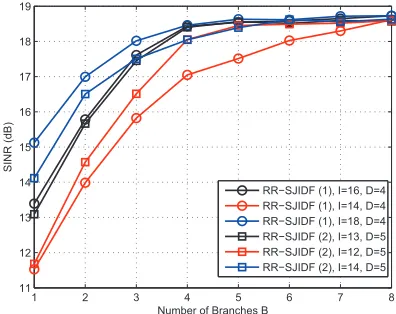
In the first several experiments, we evaluate the SINR performance of our proposed RR-SJIDF scheme with different selections ofB,I andD. We investigate RR-SJIDF scheme with the RLS algorithm in two antenna settings withM= 80

for both. The first setting is to configure the number of elements N = 10 and the number of pulsesJ = 8, and the second is to configureN = 8andJ = 10. The evaluation of the SINR performance against the number of branches B is shown in Fig. 4. We consider the RR-SJIDF-RLS algorithm with different values of I and D in both antenna settings. The results indicate that the RR-SJIDF-RLS algorithm using B = 4can achieve approximately the same performance of that using more than 4 branches. Thus, in our case, to meet the best trade-off between the performance and the complexity, we normally choose B= 4 in our simulations. In Fig. 5, the SINR performance against the rankDis shown. We can find that for the first antenna setting, the proposed scheme achieves the best performance with D= 4when I = 16and B= 4, while for the second antenna setting, the scheme achieves the best performance with D = 5 when I = 13 and B = 4. The results indicate an interesting fact that the selection of ranksDandIis highly related to the antenna setting, in other words, it is related to the structure of the received signal. That means the performance of the reduced-rank STAP algorithms can be improved if the structure of the received signal are well explored.

In the next experiment, we evaluate the SINR performance against the interpolator rank I for the proposed RR-SJIDF-RLS algorithm with different B andD, which are shown in

For R

eview Only

1 2 3 4 5 6 7 8

11 12 13 14 15 16 17 18 19

Number of Branches B

SINR (dB)

[image:12.612.337.534.59.216.2]

RR−SJIDF (1), I=16, D=4 RR−SJIDF (1), I=14, D=4 RR−SJIDF (1), I=18, D=4 RR−SJIDF (2), I=13, D=5 RR−SJIDF (2), I=12, D=5 RR−SJIDF (2), I=14, D=5

Fig. 4. SINR performance vs the number of branchesBwith different values ofIandD,M= 80,α= 0.9998,K= 100 snapshots. (1)N= 10andJ= 8

antenna setting, (2)N= 8andJ= 10antenna setting.

2 3 4 5 6

−10 −5 0 5 10 15 20

Rank D

SINR (dB)

[image:12.612.88.286.60.217.2]

RR−SJIDF (1), I=16, B=4 RR−SJIDF (1), I=14, B=4 RR−SJIDF (2), I=13, B=4 RR−SJIDF (2), I=12, B=4

Fig. 5. SINR performance vs the rankDwithM = 80,α= 0.9998,K

= 100 snapshots. (1)N = 10andJ= 8antenna setting, (2)N = 8and

J= 10antenna setting.

Fig. 6. The proposed scheme can improve the performance and converge fast if it is able to construct an appropriate subspace projection with proper coefficients in ω¯b(i) andυ¯b(i). Thus,

for this reason and to keep a low complexity we adoptI = 16

andD= 4for the first antenna setting andI= 13andD= 5

for the second antenna setting since these values yield the best performance. In the folowing subsection, we will focus on the performance assessment of the proposed STAP scheme with B= 4,I= 16andD= 4for the antenna setting I.

B. Comparison with Existing Algorithms

In this subsection, we compare both the SINR performance against the number of snapshots and the PD performance

against the signal-to-noise-ratio (SNR) for the different designs of linear receiver using the full-rank filter with the RLS algorithm, the MSWF with the RLS algorithm, the AVF and our proposed technique, where the reduced-rank filter ω¯(i)

10 12 14 16 18 20

10 11 12 13 14 15 16 17 18 19 20

Interpolator Rank I

SINR (dB)

RR−SJIDF(1), B=4,D=4 RR−SJIDF(1), B=3,D=4 RR−SJIDF(2), B=4,D=5 RR−SJIDF(2), B=3,D=5

Fig. 6. SINR performance vs the interpolator rankI withM = 80,α= 0.9998,K = 100 snapshots. (1)N = 10 andJ = 8antenna setting, (2)

N= 8andJ= 10antenna setting.

0 100 200 300 400 500

0 2 4 6 8 10 12 14 16 18 20

Snapshot

SINR (dB)

Reduced Rank STAP

Full−Rank−LCMV−RLS JDL−RLS (5×3) AVF, D=8 MSWF−RLS,D=6

RR−SJIDF−RLS, B=1,I=16,D=4 RR−SJIDF−RLS, B=2,I=16,D=4 RR−SJIDF−RLS, B=4,I=16,D=4 RR−SJIDF−CCG, B=4,I=16,D=4 MVDR

Fig. 7. SINR performance against snapshot withM= 80, SNR = 0 dB,α= 0.9998. All algorithms are initialized to a scaled identity matrixδ−1_{I, where}

δis a small constant.

withDcoefficients provides an estimate to determine whether the target is present or not.

Firstly, as shown in Fig. 7, we evaluate the SINR against the number of snapshots K performance of our proposed algorithm with different setting parameters and compare with the other schemes. The schemes are simulated overK= 500

snapshots and the SNR is set at 0 dB. The curves show an excellent performance by the proposed algorithm, which also converges much faster than other schemes. With the number of branchesB= 4, the proposed scheme approaches the optimal MVDR performance after 50 snapshots. As one may expect, with an increase in the number of branches, the steady SINR performance improves.

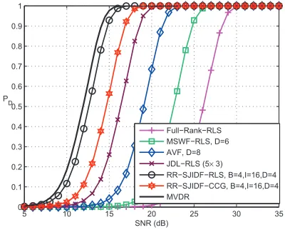
In the second experiment, in Fig. 8, we present PD versus

SNR performance for all schemes using 50 snapshots as the training data. The false alarm rate PF A is set to 10−6 and

we suppose the target is injected in the boresight (0◦) with Doppler frequency 100Hz. The figure illustrates that the

[image:12.612.88.539.278.443.2]

For R

eview Only

5 10 15 20 25 30 35

0 0.1 0.2 0.3 0.4 0.5 0.6 0.7 0.8 0.9 1

P_D

SNR (dB)

Full−Rank−RLS MSWF−RLS, D=6 AVF, D=8 JDL−RLS (5× 3)

[image:13.612.88.288.59.220.2]

RR−SJIDF−RLS, B=4,I=16,D=4 RR−SJIDF−CCG, B=4,I=16,D=4 MVDR

Fig. 8. Probability of detection performance vs SNR withM = 80,α= 0.9998,K= 50 snapshots,PF A= 10−6.

−1500 −100 −50 0 50 100 150

2 4 6 8 10 12 14 16 18 20

Doppler Frequency (F_D)

SINR (dB)

Full−Rank−RLS JDL−RLS AVF MSWF−RLS RR−SJIDF−CCG RR−SJIDF−RLS Optimal

Fig. 9. SINR performance against Doppler frequency (FD) withM = 80,

α= 0.9998,K= 100 snapshots.

posed algorithm provides sub-optimal detection performance using very short support data, but remarkably, obtains a 90 percent detection rate, beating 50 percent for the AVF, 40 percent for the MSWF with the RLS and 30 percent for the full rank filter with the RLS at an SNR level of 15 dB.

We evaluate the SINR performance against the target Doppler frequency at the main bean look angle for our proposed algorithms and other existing algorithms, which are illustrated in Fig. 9. The potential Doppler frequency space form -150 to 150 Hz is examined and 100 snapshots are used to train the filter. The plots show that our proposed algorithms converge and approach the optimum in a short time, and form a deep null to cancel the mainbeam clutter. Note that the proposed RR-SJIDF-RLS algorithm outperforms other algorithms in the most of Doppler bins, but performs slightly worse than the AVF algorithm in the Doppler range of -50 to 50Hz.

VII. CONCLUSIONS

In this paper, we proposed an RR-SJIDF STAP scheme for airborne radar systems. The proposed scheme performed dimensionality reduction by employing a MPB framework, which jointly optimizes interpolation, decimation and filtering units. The output was switched to the branch with the best performance according to the minimum variance criterion. In order to design the decimation unit, we considered the optimal decimation scheme and also a low-complexity pre-stored dec-imation units scheme. Furthermore, we developed an adaptive RLS algorithm for efficient implementation of the proposed scheme. Simulations results showed that the proposed RR-SJIDF STAP scheme converged at a very fast speed and provided a considerable SINR improvement, outperforming existing state-of-the-art reduced-rank schemes.

REFERENCES

[1] L. E. Brennan and I. S. Reed, “Theory of adaptive radar”, IEEE Trans. Aero. Elec. Syst., vol. AES-9, no. 2, pp. 237–252, 1973.

[2] I. S. Reed, J. D. Mallett, and L. E. Brennan, “Rapid convergence rate in adaptive arrays”,IEEE Trans. Aero. Elec. Syst., vol. AES-10, no. 6, pp. 853–863, 1974.

[3] E. J. Kelly, “An adaptive detection algorithm”, IEEE Trans. Aero. Elec. Syst., vol. AES-22, no. 2, pp. 115–127, 1986.

[4] A. M. Haimovich and Y. Bar-Ness, “An eigenanalysis interference canceler”,IEEE Trans. Sig. Process., vol. 39, no. 1, pp. 76–84, 1991. [5] F. C. Robey, D. R. Fuhrmann, E. J. Kelly, and R. Nitzberg, “A CFAR

adaptive matched filter detector”,IEEE Trans. Aero. Elec. Syst., vol. 28, no. 1, pp. 208–216, Jan 1992.

[6] J. Ward, “Space-time adaptive processing for airborne radar,”,Tech. Rep. 1015, MIT Lincoln lab., Lexington, MA, Dec. 1994.

[7] A. Haimovich, “The eigencanceler: adaptive radar by eigenanalysis methods”, IEEE Trans. Aero. Elec. Syst., vol. 32, no. 2, pp. 532–542, 1996.

[8] J. S. Goldstein and I. S. Reed, “Reduced-rank adaptive filtering”,IEEE Trans. Sig. Process., vol. 45, no. 2, pp. 492–496, 1997.

[9] J. S. Goldstein and I. S. Reed, “Theory of partially adaptive radar”,IEEE Trans. Aero. Elec. Syst., vol. 33, no. 4, pp. 1309–1325, 1997. [10] Y.-L. Gau and I.S. Reed, “An improved reduced-rank CFAR space-time

adaptive radar detection algorithm”,IEEE Trans. Sig. Process., vol. 46, no. 8, pp. 2139–2146, Aug 1998.

[11] I. S. Reed, Y. L. Gau, and T. K. Truong, “CFAR detection and estimation for STAP radar”,IEEE Trans. Aero. Elec. Syst., vol. 34, no. 3, pp. 722– 735, 1998.

[12] J. S. Goldstein, I. S. Reed, and P. A. Zulch, “Multistage partially adaptive STAP CFAR detection algorithm”, IEEE Trans. Aero. Elec. Syst., vol. 35, no. 2, pp. 645–661, 1999.

[13] J. R. Guerci, J. S. Goldstein, and I. S. Reed, “Optimal and adaptive reduced-rank STAP”, IEEE Trans. Aero. Elec. Syst., vol. 36, no. 2, pp. 647–663, 2000.

[14] R. Klemm, Principle of space-time adaptive processing, IEE Press, Bodmin, UK, 2002.

[15] W. L. Melvin, “A STAP overview”,IEEE Aero. .Elec. Syst. Mag., vol. 19, no. 1, pp. 19–35, 2004.

[16] S. Haykin,Adaptive Filter Theory, NJ: Prentice-Hall, 4th, ed2002. [17] J. S. Goldstein and I. S. Reed, “Subspace selection for partially adaptive

sensor array processing”, IEEE Trans. Aero. Elec. Syst., vol. 33, no. 2, pp. 539–544, 1997.

[18] J. S. Goldstein, I. S. Reed, and L. L. Scharf, “A multistage representation of the wiener filter based on orthogonal projections”, IEEE Trans. Inf. Theory, vol. 44, no. 7, pp. 2943–2959, 1998.

[19] D. A. Pados and S. N. Batalama, “Joint space-time auxiliary-vector filtering for DS/CDMA systems with antenna arrays”, IEEE Trans. Commun., vol. 47, no. 9, pp. 1406–1415, 1999.

[20] D. A. Pados and G. N. Karystinos, “An iterative algorithm for the computation of the MVDR filter”, IEEE Trans. Sig. Process.], vol. 49, no. 2, pp. 290–300, Feb 2001.

[21] D. A. Pados, G. N. Karystinos, S. N. Batalama, and J. D. Matyjas, “Short-data-record adaptive detection”,2007 IEEE Radar Conf., pp. 357– 361, 17-20 April 2007.

[image:13.612.86.292.248.444.2]

For R

eview Only

[22] H. Wang, and L. Cai, “On adaptive spatial-temporal processing for airborne surveillance radar systems”,IEEE Trans. Aero. Elec. Syst., vol. 30, no. 3, 660670, 1994.

[23] R. S. Adve, T. B. Hale, and M. C. Wicks, “Practical joint domain localised adaptive processing in homogeneous and nonhomogeneous environments. Part 1: Homogeneous environments.”, IEE Proceedings Radar, Sonar and Navigation, vol. 147, no. 2, 5765, 2000.

[24] R. S. Adve, T. B. Hale, and M. C. Wicks, “Practical joint domain localised adaptive processing in homogeneous and nonhomogeneous environments. Part 2: Nonhomogeneous environments.”,IEE Proceedings Radar, Sonar and Navigation, vol. 147, no. 2, 6674, 2000.

[25] R. C. de Lamare and R. Sampaio-Neto, “Reduced-rank adaptive filtering based on joint iterative optimization of adaptive filters”,IEEE Sig. Proc. Lett., vol. 14, no. 12, pp. 980–983, 2007.

[26] R. Fa, R. C. de Lamare, and D. Zanatta-Filho, “Reduced-rank STAP algorithm for adaptive radar based on joint iterative optimization of adaptive filters”, inConf. Record of the Fourty-Second Asilomar Conf. Sig. Syst. Comp., 2008.

[27] R. C. de Lamare and R. Sampaio-Neto, “Adaptive reduced-rank mmse parameter estimation based on an adaptive diversity-combined decimation and interpolation scheme”, inProc. IEEE Int. Conf. Acous. Speech Sig. Process., 15–20 April 2007, vol. 3, pp. III–1317–III–1320.

[28] R. C. de Lamare, and R. Sampaio-Neto, “Adaptive reduced-rank processing based on joint and iterative interpolation, decimation, and filtering”, IEEE Trans. Sig. Process., vol.57, no.7, pp.2503-2514, July 2009

[29] S. Applebaum and D. Chapman, “Adaptive arrays with main beam constraints”, IEEE Trans. on Ant. Prop., vol. 24, no. 5, pp. 650–662, 1976.

[30] G. H. Golub and C. F. van Loan,Matrix Computations, Wiley, 2002. [31] L. S. Resende, J. M. T. Romano, and M. G. Bellanger, “A fast

least-squares algorithm for linearly constrained adaptive filtering”,IEEE Trans. Sig. Process., vol. 44, no. 5, pp. 1168–1174, 1996.

[32] Jr. Apolinario, J. A., M. L. R. De Campos, and C. P. Bernal O, “The constrained conjugate gradient algorithm”,Signal Processing Letters,vol. 7, no. 12, pp. 351–354, 2000.

[33] P. S. Chang and Jr. A. N. Willson, “Analysis of conjugate gradient algorithms for adaptive filtering”,IEEE Trans. Sig. Process., vol. 48, no. 2, pp. 409–418, Feb. 2000.

[34] M. E. Weippert, J. D. Hiemstra, J. S. Goldstein, and M. D. Zoltowski, “Insights from the relationship between the multistage wiener filter and the method of conjugate gradients”, in Proc. Sensor Array and Multichannel Signal Processing Workshop, 4–6 Aug. 2002, pp. 388–392. [35] L. L. Scharf, E. K. P. Chong, M. D. Zoltowski, J. S. Goldstein, and I. S. Reed, “Subspace expansion and the equivalence of conjugate direction and multistage wiener filters”,IEEE Trans. Sig. Process., vol. 56, no. 10, pp. 5013–5019, Oct. 2008.

[36] L. Wang and R. C. de Lamare, “Constrained adaptive filtering algorithms based on conjugate gradient techniques for beamforming,” Submitted to

IET Signal Processing.

[37] H. L. Van Trees, Optimum Array Processing, Wiley, New York, 2002.