Rochester Institute of Technology
RIT Scholar Works
Theses Thesis/Dissertation Collections
5-1-2009
Feature selection of microarray data using genetic
algorithms and artificial neural networks
Paul Yacci
Follow this and additional works at:http://scholarworks.rit.edu/theses
This Thesis is brought to you for free and open access by the Thesis/Dissertation Collections at RIT Scholar Works. It has been accepted for inclusion in Theses by an authorized administrator of RIT Scholar Works. For more information, please [email protected].
Recommended Citation
Feature Selection of Microarray Data Using
Genetic Algorithms and Artificial Neural
Networks
Approved:
________________________________
Director of Bioinformatics
________________________________
Head, Department of Biological Sciences
Submitted in partial fulfillment of the requirements for the Master of Science
degree in Bioinformatics at the Rochester Institute of Technology.
Paul Yacci
Thesis Committee
Members
Dr. Roger Gaborski Department of Computer Science Laboratory for Computational Studies Rochester Institute of Technology, Rochester NY
Dr. Anne Haake
Department of Information Sciences and Technologies Rochester Institute of Technology, Rochester NY
Dr. Gary Skuse Director of Bioinformatics
ABSTRACT
Microarrays, which allow for the measurement of thousands of gene expression
levels in parallel, have created a wealth of data not previously available to biologists
along with new computational challenges. Microarray studies are characterized by a low
sample number and a large feature space with many features irrelevant to the problem
being studied. This makes feature selection a necessary pre-processing step for many
analyses, particularly classification. A Genetic Algorithm -Artificial Neural Network
(ANN) wrapper approach is implemented to find the highest scoring set of features for an
ANN classifier. Each generation relies on the performance of a set of features trained on
an ANN for fitness evaluation. A publically-available leukemia microarray data set
(Golub et al., 1999), consisting of 25 AML and 47 ALL Leukemia samples, each with
7129 features, is used to evaluate this approach. Results show an increased performance
List of Figures
Figure 1 A simplified view of the central dogma of molecular biology. ... 2
Figure 2 Hematopoiesis. ... 4
Figure 3 Leukemia cells ... 5
Figure 4 Hybridization ... 7
Figure 5 Affymetrix® PM MM strategy ... 9
Figure 6. Normalized gene expression values for 50 genes from (Golub 1999) ... 10
Figure 7 Signal to noise distribution. ... 13
Figure 8 A Simple diagram of a perceptron. ... 18
Figure 9 Sample transfer/activation functions, http://www.mathworks.com/ ... 19
Figure 10 Basic architecture of an artificial neural network ... 19
Figure 11 Simple genetic algorithm ... 24
Figure 12 Probability vector ... 27
Figure 13 Crossover operator ... 28
Figure 14 Chromosome decoding ... 31
Figure 15 Sampling distributions of ANN performance, 10, 25 and 100 samples ... 34
Figure 16 Structure of ANN ... 33
Figure 17 Fitness of population over 131 generations ... 40
Acknowledgments
I would like to thank my committee members who have helped make this thesis a
success. I am also grateful for all of the support and encouragement from my family and friends, without which, this thesis would not have been possible.
Introduction
Central Dogma
To fully understand this study, a basic knowledge of molecular biology and the data used
is necessary. At the heart of gene expression and cell biology is the Central Dogma. The central
dogma has influenced molecular biology since it was first described by Crick in 1956 (Watson,
et al. 2004). Simply, information is stored in DNA which passes through an intermediate
molecule named mRNA to construct a protein as in Figure 1.
Figure 1 A simplified view of the Central Dogma of molecular biology.
DNA which has been described as the ‘blueprint’ of life is the initial source of
information. In eukaryotic organisms DNA is located in the nucleus of cells. A DNA sequence
can be thought of as a string of characters consisting of the letters, A, T, C and G. These are
representations of the bases, Adenine, Thymine, Cytosine, and Guanine. An organization of
these bases that expresses a polypeptide results in a gene. While the exact definition of a gene is
still debated amongst experts in the field, it can be understood as a substring of the entire DNA
groups of three bases, together which code for an amino acid. However the DNA does not leave
the nucleus; it serves as a “permanent” memory that is accessed for its information and returned
for storage. In order to convert the information contained within a string of DNA to a functional
protein, the sequence must first be converted into an intermediate molecule known as mRNA.
Chemically mRNA differs in its backbone structure and its base usage (DNA uses Thymine,
mRNA uses Uracil). The “m” in mRNA stands for messenger, which accurately describes its
purpose. A series of enzymes read the DNA sequence and transcribe the DNA sequence into an
mRNA molecule. The mRNA molecule serves as an inverse mobile copy of the DNA sequence.
The mRNA exits the nucleus of the cell where it is translated into a polypeptide by complexes of
molecules in the cytoplasm called ribosomes. These polypeptides go on to perform different
functions throughout the cell. One of the important roles these polypeptides play is in complex
feedback loops that regulate the amount of themselves or other polypeptides; making cellular
processes and regulation a complex web of non linear interactions.
Cancer
Cancer has afflicted humans throughout recorded history, with some of the earliest
documented cases found in ancient Egyptian mummies (American Cancer Society, 2009).
Cancer arises through several small accumulated mutations or a few large disruptions within the
genetic material of cells (Hagemeijer & Grosveld, 1996). These mutations can arise from DNA
replication errors or through environmental effects such as radiation and chemical exposure.
Cellular division is the process that converts a single fertilized egg into an organism with
billions or trillions of cells. Normally cellular division is a tightly controlled process, where
several systems ensure that cells divide only when appropriate. However, if a cell collects
enough mutations in these control systems over time, problems will arise and the cell will no
longer possess the ability to control its cellular division. This results in an increase in aberrant,
often non-functional cells, which can form a tumor. The different subtypes of cancer derive
from their tissues of origin. For examples lung cancers arise from mutated lung cells and skin
cancer from skin cells. While all cells within an organism originally arise from a single cell,
these cells undergo differentiation that result in physiologically different cells. When these cells
of different lineages become diseased they can become unique forms of cancer.
Leukemia is a common cancer of the blood caused by diseased cells from an organism’s
immune system. Approximately 231,641 people in the United States suffer from this disease
(Leukemia and Lymphoma Society, 2009). The two predominate forms of leukemia are Acute
Myelogenous Leukemia and Acute Lymphoblastic Leukemia. Both Acute Myelogenous
Leukemia (AML) and Acute Lymphoblastic Leukemia (ALL) are characterized by increases in
circulating non functional immune precursor cells.
Leukemia cells arise from progenitor cells that normally undergo hematopoiesis.
Hematopoiesis is the differentiation process that results in the different cell types of the immune
system. As a cell further divides in a differentiation pathway, its function becomes more
specialized. All of cells of the immune system start as a multipotential hematopoietic stem cell
and then further differentiate into their specific cell types. Stem cells retain the ability to
differentiate into a specific type of cell. While they can also renew themselves the hematopoietic
Figure 2 Hematopoiesis two major lineages, Lymphoid and Myeloid.
The myeloid lineage gives rise to cells such as granulocytes, phagocytes and monocytes
(Parham, 2005). These cells primarily function as part of the innate immune response. Cells of
the innate immune response serve as the first responders to threats to the body. This is
contrasted to the lymphoid lineage which differentiates into B cells and T cells which are the key
components of the adaptive immune response, which tailors antibodies to fight infections. AML
and ALL, respectively, refer to unregulated division of a myeloid lineage cell or a lymphoid
lineage cell.
Once these cells have lost the ability to control their division, they rapidly dominate the
blood stream. This is contrasted with CML and CLL which are the chronic forms of disease that
typically have a slower progression, and often arise from cancerous cells that are further
Importance of Diagnostic Tests
In prescribing treatment for these cancers, accurate diagnostic tests play an important
role. Without knowing the specific type of cancer, important decisions about treatment regimes
are difficult for a doctor to make. Due to the difference in origin, the cancerous cells respond
differently to treatments and clinical outcome can vary (Poi & Evans, 1998). Therapies that are
tailored for AML do not work as well against ALL and vice versa, resulting in differences in
patient outcome. In the information age and with the future vision of personalized medicine,
knowing specific details about a cancer can result in a much different prognosis and treatment.
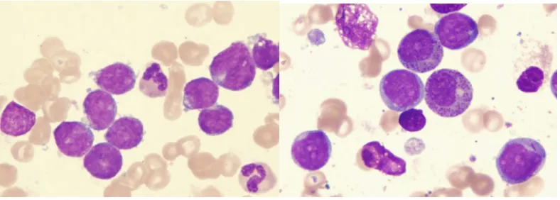
[image:11.612.109.503.470.611.2]Leukemia cells are traditionally difficult to classify by morphology alone as seen in
Figure 3, and require a series of immunological tests to determine their nature. However these tests remain inaccurate by making diagnosis a subjective task. Microarray profiling of cancer
cells has been suggested as a more informative approach to diagnosis (Golub et al., 1999)
ALL AML
Microarrays
Biologists are particularly interested in the types and amounts of proteins present within
the cell under given conditions. Because proteins act as the functional molecules of a cell,
having different types and quantities changes the behavior of the cell. In cancer this is of even
greater interest, as cancers have different expression patterns. However, measuring the amount
of a specific protein remains a complicated process. This is due to the complex,
three-dimensional structures of proteins. A protein structure can be flexible and can vary greatly in
shape and size, making high throughput measurement difficult (Primrose & Twyman, 2004). To
help infer the proteins present in a cell under given conditions, researchers measure mRNA.
Since mRNA is a precursor for protein, it can be assumed with some confidence that the quantity
of mRNA is proportional to the quantity of protein present. The relationship is not always 1-to-1
requiring further validation using protein studies.
Although it is a labile macromolecule, the structure of mRNA lends it to much easier
measurement than protein. Every protein is unique, making it difficult to design a tool that can
measure thousands of proteins simultaneously. Nucleic acids are able to hybridize to their
complementary sequence. Hybridization is the binding of complementary molecules in a low
energy state that creates a double stranded molecule that does not easily separate. In
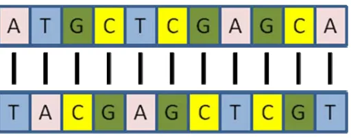
hybridization, Adenine binds with Thymine and Cytosine binds with Guanine (Figure 4). This
highly specific molecular interaction allows for massive parallel comparison of thousands of
Figure 4 Hybridization between two DNA molecules
When preparing a microarray, first mRNAs are isolated from a given sample representing
a state of interest (cancer, non-cancer etc.) and reverse transcribed and labeled with a fluorescent
tag. Reverse transcription is the process of converting mRNA back into DNA, a more stable
information carrier, using mRNA dependent DNA polymerase or reverse transcriptase.
This solution of reverse transcribed cDNA, known as the target, is then washed over the
array and sequences are allowed to hybridize to the probes. After hybridization, the remaining
single stranded sequences are washed away, leaving only sequences that have found a
complement among the probe sequences bound to the array. The amount of double stranded
DNA is then measured by the fluorescence intensities of the hybridized sequences for each
location on the array.
There exist several forms of microarray, one of the most popular being Affymetrix
GeneChip®. An Affymetrix GeneChip® microarray contains thousands of individual DNA
sequences called probes, affixed to the surface of a quartz wafer using photolithographic
techniques (Draghici, 2003). These probes contain the known complement to thousands of genes
The expression values for a gene from Affymetrix® data actually represent an average of
20 different probes pairs. A probe pair consists of one perfect match (PM) probe and one
mismatch (MM) probe. The perfect match regions are sequences that are perfectly
complementary to a target sequence. A mismatch contains the same sequence as the PM, except
that it contains exactly one base difference in the middle of the probe and is considered to be a
measurement of non-specific hybridization (Draghici, 2003). This technique allows for
correction of intensities to determine a more accurate measurement of the true amount of cRNA
present. Ideally the PM intensity is much greater than the MM intensity, allowing for a clear
signal.
Equation 1
PM represents the perfect match probe intensity, MM the mismatch probe intensity, N the number of probe
Figure 5 Affymetrix® PM MM strategy
The main benefit from microarray technology is the high throughput measurement of
thousands of genes in parallel. In the past, technologies such as the Northern blot analysis and
real time PCR could only be used to quantify the expression of a handful of genes at a given time
(Kuo, et al., 2004). However a common problem in microarray data analysis is the small number
of replicates. This stems from the huge imbalance between the number of features (probes) and
the number of samples.
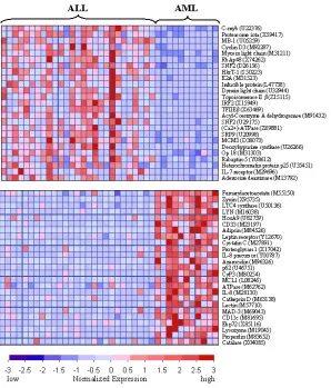
Traditionally microarray data has been analyzed using clustering techniques. From this, a
visual approximation is typically taken to determine if there is indeed a pattern present that
warrants further study. As microarray data is noisy, it can sometimes be difficult to determine
where these patterns exist. The clustering results are typically represented in what is called a
samples, and the y axis represents the genes analyzed. This representation allows for quick
[image:16.612.191.489.141.490.2]visual interpretation of intensities that is easily interpretable by the human eye.
Figure 6. Normalized gene expression values for 50 genes, represented as a heatmap from (Golubet al., 1999).
Feature Subset Selection
Feature subset selection (FSS) is a well studied problem within the machine learning
community. This problem is characterized by a dataset with a large number of features. Within
this set of features there are a few features that contain relevant information, with the rest of the
reducing the number of features that are ultimately used for classification, an increase in
performance in the algorithm can be seen (Yang & Honavar, 1998). Filter and wrapper
approaches are the two primary methods that researchers utilize to tackle this problem. The
important difference between filter and wrapper methods is their use of univariate and
multivariate analysis, respectively.
The filter approach performs feature selection as a preprocessing step before the use of a
classification algorithm (Yang & Honavar, 1998). Here each feature is evaluated independently
using a test statistic and acceptable features are used for the classification algorithm. Studies of
feature reduction of microarray data most commonly use this approach (Inza et al. 2004). A
commonly used test statistic in microarray studies is the t-test to isolate significantly
differentially expressed genes.
The wrapper approach is any method that incorporates a classifier to select relevant
features as a group (Yang & Honavar, 1998). Groups of features are evaluated together using an
algorithm, and the best set of features is retained before modifying the feature set. This
approach, while generally more accurate than the filter approach, comes at a computational cost
(Inza et al. 2004). The wrapper method relies on many evaluations of the data while the filter
approach uses a single evaluation.
Dataset
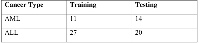
Within the microarray data mining community the Golub dataset (Golub et al., 1999) is
often used as a standard for evaluating new algorithms. The data is presented as a training set of
38 samples and an independent testing set of 34 samples. Each of these is represented in an n x
contains the expression values for each sample at each feature. The samples represent two types
[image:18.612.136.480.181.256.2]of leukemia, acute myeloid leukemia (AML) and acute lymphoblastic leukemia (ALL).
Table 1
Cancer Type Training Testing
AML 11 14
ALL 27 20
Original data division from Golub 1999
Golub et al. (1999) developed a class prediction algorithm that achieved an accuracy of
85% for samples presented and 100% for samples that were above a prediction strength
threshold. This method first identified samples that were significantly differentially expressed
by a signal to noise statistic. This statistic compares the average expression between two classes
and looks for a high difference, representing high correlation between the gene and an idealized
expression pattern of high expression in one class and low expression in the other.
Equation 2
µ1=mean of genes in class 1, µ2=mean of genes in class 2, σ1= standard deviation of genes in class 1,σ2=standard
deviation of genes in class 2
A positive value reflects gene expression that is high in class 1 and low in class 2,
whereas a negative value represents gene expression that is high in class 2 but low in class 1.
between -1 and 1 like a Pearson correlation. The genes were then ranked based on this statistic.
The set of n informative genes is constructed from genes that are most highly correlated to
high expression in class one and genes that are most highly correlated to high expression in
[image:19.612.125.495.202.513.2]class two.
Figure 7 Signal to noise distribution. Negative values indicate a strong correlation to high expression in ALL samples one
and low expression in AML samples. Positive values indicate a strong correlation to low expression ALL samples and
high expression in AML samples.
From the set of informative genes from the training class a classifier was constructed.
Equation 3
=Correlation, =Expression of gene, =
The sum of the absolute values of the vote for each class is calculated to give the final
prediction. The winning class is determined by the most votes. A larger difference in votes
yields higher prediction strengths.
Equation 4
This model made strong predictions about most of the independent samples presented; it
did not classify five of the samples above the set prediction strength threshold of 0.3, resulting in
samples labeled “no call”. Of the 34 independently tested samples, only 29 met or exceeded the
threshold for prediction. Therefore, it would be more accurate to claim that this technique
classified correctly for ~85% of the samples that were presented to it. Of the five samples that
did not meet the prediction threshold, two did not correctly classify. Golub et al.’s 1999 report
of 100% accuracy is misleading and should be more properly reported as 100% accuracy of
samples that exceeded the threshold.
While they showed that there was sufficient information contained within the data to
classify, they did not attempt to determine the minimum number of features for accurate
prediction. Ultimately Golub chose a subset of 50 genes to use as predictive features. However,
genes obtained the same percent accuracy (Golub et al., 1999). Whether this represents a
classification ability higher than the original 85%, remains unreported.
The number of samples within this dataset is adequate for accurate prediction according
to Dobbin (Dobbin, Zhao, Simon, 2008) who created a new method to determine required
sample sizes based on the maximum standardized fold change of the dataset. Fold change is the
ratio of the experimental group expression to the baseline group expression. Dobbin uses
Equation 5 to determine fold change for a gene.
Equation 5
B=Baseline group mean and E=Experimental Group mean
Using this method only 28 samples are required for a training set to produce an accurate
classifier (Dobbin et al. 2008).
Samples that are vastly different will require fewer features to classify on, and samples
that are most similar will require more complex feature subsets to classify on. The signal
intensity patterns of the Golub dataset are expected to have a large number of features to classify
upon. (Dobbin, Zhao, Simon, 2008).
Normalization
To correct for intensity differences, Golub et al. (1999) used several normalization
steps. First a rescaling method based on regression was used to rescale the samples. This
sample. The inverse of the slope is used as a multiplicative rescaling factor by which the data is
multiplied by. The closer a rescaling factor is to 1 the more similar it was to the reference
sample. For all samples within the Golub dataset, the greatest rescaling factor is 3.091.
Additional preprocessing steps include (Dudoit, Fridlyand, & Speed, 2002):
1)
Equation 6
Setting a minimum value of 100 and maximum value of 16000 for all expression
measurements
2)
Equation 7
Removing features that the maximum /minimum expression values for a gene are less
than or equal to 5 or where difference between the maximum and minimum values is
less than 500.
Equation 8
After performing these steps, 3051 features remained (Dudoit, Fridlyand & Speed,
2002). These were then used to calculate the signal to noise statistic (Dudoit, Fridlyand,
& Speed, 2002). Max and min refer to the maximum and minimum expression value
respectively, for an individual gene.
Neural networks
Artificial Neural Networks (ANNs) are an attempt to model the power of the brain (Baldi
& Brunak, 2001). The brain has evolved many efficient ways to store and process information
that we attempt to model through artificial neural networks.
The Neuron
Artificial neural networks had their start relatively recently in the 1940’s. The basic
processing unit of a neural network is the neuron. The first model of the neuron was published
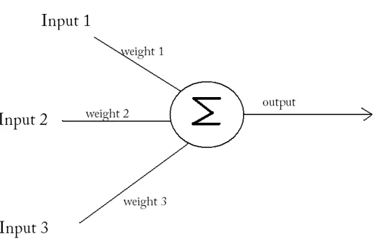
by McCullough and Pitts in 1943 (Trappenberg, 2002). At the highest level a neuron receives a
series of inputs and depending upon the strength of the input and the connection determines
whether the neuron will fire or not. The inputs are multiplied by their synaptic connection and
summed. This sum is then used as input for a transfer function which calculates the output of the
neuron. This function is represented in Equation 9. The basic conceptual framework for a single neuron is show in Figure 8.
w represents the weight of the synaptic connection between the input and the neuron, r represents the input
[image:24.612.190.459.226.400.2]value. g represents the transfer function of the neuron.
Figure 8 A Simple diagram of a perceptron. Lines represent connections to other neurons (synapses).
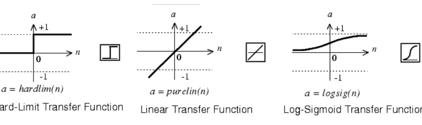
Each neuron utilizes a transfer function that determines a neurons response to the sum of
its inputs. Early neuronal models such as the McCullough Pitts neuron utilized a hard limit
transfer function that produced a binary response if a threshold was met. However newer models
utilize continuous functions that allow for finer adjustments in neuronal output. Some
Figure 9 Sample transfer/activation functions. Different usage will give the network different dynamics. (From
http://www.mathworks.com/)
These different transfer functions result in different neuron output. For example a hard
limit function will only propagate a 1 or a 0, revealing little information to how accurate the
neuron is but resulting in very clear propagation of signal. Whereas a continuous transfer
function is much more precise with outputs but can potentially propagate irrelevant signals.
Figure 10 Basic architecture of an artificial neural network. Input neurons take in supplied values and connect to one or
more hidden layers. This hidden layer can connect to another hidden layer or to an output layer depending on the
[image:25.612.173.475.413.624.2]The basic architecture of an artificial neural network is seen in Figure 10. Each circle represents a single neuron as seen in Figure 8, where the output of each serves as an input into the next layer. This connection of simple neurons was first implemented in the perceptron model by
Rosenblatt in 1958. The connections between neurons represent a weighted connection called a
synapse. Like the single neuron seen the inputs are multiplied by the synaptic weight and passed
through a transfer function. A typical ANN consists of an input layer, k hidden layers, and an
output layer. This network topology is determined by the user and is based on the type and
complexity of the problem space.
Training
Training is an iterative process that seeks to modify the network through numerous
presentations of data. There are many different methods to train neural networks, the two main
distinctions are unsupervised and supervised learning. An unsupervised neural network only
uses the input data to adjust its synaptic weights. Supervised learning however relies on a set of
training data with known target values. In other words, the training data consists of a set of input
patterns and output values. The goal of training is to optimize a function that will map the inputs
to the outputs that can be used to correctly approximate unseen inputs.
Constructing an ANN using a supervised learning methodology requires the initialization
of a network with random synaptic weights between neurons. At this point an input signal
presented to the network would result in no meaningful output. To derive a meaningful output
the network synapses must be adjusted. The method to adjust the many weights of the network
requires a calculation of error of the network for an input pattern at each epoch. An epoch
response. The error of the network for a given input pattern is described as the difference
between the network output and the desired output value. A standard error measure, such as
mean squared error is often used to describe this distance.
Equation 10
While this error value shows how far the network output is from a desired value, it does
not reveal anything about how to correct the network to more closely match the desired value.
To minimize the error value, the error is used in a learning function to update the synaptic
connections of the network. A simple synaptic learning function is shown in Equation 11
Equation 11
wnew represents the new weight of the input neuron, wold the old weight of the neuron, alpha the learning
rate, targetValue-output is the error function and the input is the input that goes through the synapse
A learning rate is often used to control how quickly the weights are updated. If a large
value is used the weights of the network will oscillate wildly if set too low it will take more
epochs to adjust the weights.
Several learning paradigms exist to train networks, one of the most commonly used is
backpropagation. Backpropagation originally described in 1974 by Paul Werbos (Chester, 1993)
is an extension of Equation 11. Simple learning methods are not able to directly compute the error from hidden layers of multilayered networks; however with the discovery of
topologies that were previously unavailable. Backpropagation is accomplished through a process
where error correction flows through the network in a reverse direction (Swamy, 2006).
Backpropagation attempts to minimize the amount of error by modifying the synapses with the
strongest connections. The weights of these synapses are then modified to a greater degree than
their weaker counterparts using a method similar to Equation 11.
Testing
After training has been completed, usually signaled by a lack of further decrease in the
error or after a set number of epochs, the weights of the network are set and testing of new
samples begins. During testing the testing data is presented to the network to obtain a measure
of performance. This performance is measured by a similar method that is used to determine the
error of the network during training.
Cross validation
An important part in evaluation of any classifier is the use of cross validation. However
with microarray data this is difficult, as typically there are a statistically small number of
samples, making over fitting of the model a real possibility. Some basic cross validation
techniques include, leave one out, hold out and k-fold.
Leave one out cross validation is one of the most extreme cross validation methods. In
this case, 1 sample is used for testing and n-1 samples are used for training. This is repeated n
times, until all individuals have taken a turn as the testing sample. This is a nearly unbiased
method rapidly grows with larger sample sizes. With 72 samples, this would take 72 repeat
evaluations to build a fitness value.
The n-fold cross validation method is a scaled down version of the leave one out method,
where the dataset is divided into n divisions. Each of these divisions is used as a testing set
while the classifier is trained on the remaining samples.
Hold out cross validation is commonly used for classifiers that have a low number of
samples. Typically in this case, 90% of the samples are used for training and the remaining 10%
are used for testing procedures.
While supervised artificial neural networks are powerful tools by themselves they can
only sort what is presented to them. The typical structure of microarray data has too many
features and not enough replicates. To alleviate this problem, a Genetic Algorithm (GA) can be
used to evaluate combinations of genes.
Genetic Algorithms
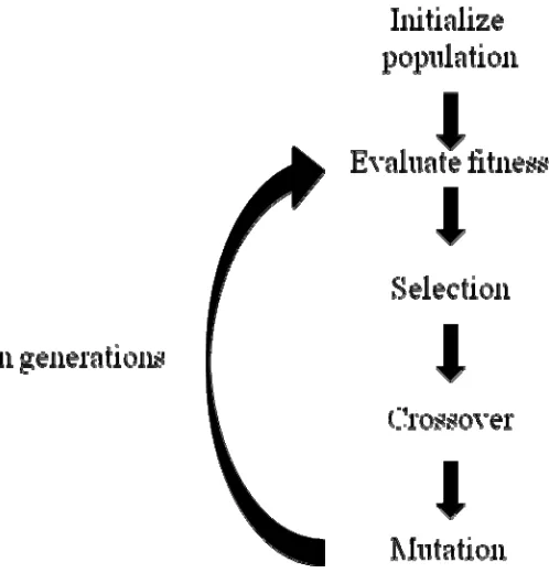
Genetic algorithms comprise a search algorithm that guides its search based on a model
of evolution (Mitchell, 1999). Evolution is the process by which organisms continually improve
over generations, through, selection, crossover and mutation. Evolution derives its power by
evaluating many possible solutions at once, and propagating the fittest.
In a genetic algorithm, a population of organisms is represented by a population of short
strings called chromosomes. Each chromosome represents a different portion of the possible
of features for a given problem. One could evaluate every possible solution for a problem,
known as a brute force approach, but as the number of parameters increases the search space
grows in dimensionality, resulting in problem spaces that are too large to search with exhaustive
methods. Genetic algorithms have been shown to be a robust search method for problems with
extremely large search spaces (Goldberg, 1989). Within a search space there are often many
local minima/maxima and one global minima/maxima. Local minima/maxima are solutions that
are close but are not the best solution. Minima or maxima are substituted depending on the
direction that function is being optimized. Many optimization algorithms go to great lengths to
avoid or escape local solutions. The global solutions represent the best possible solution and are
[image:30.612.182.431.400.660.2]often difficult to find.
Representation
The choice of representation in a genetic algorithm is of utmost importance; this process
involves mapping parameters into a string that the algorithm can manipulate. Poor choice of
representation can limit how the algorithm works (Reeves & Wright,1995).
Many Genetic algorithms utilize a binary representation of the data (Sivanandam and
Deepa). In a feature selection problem this would consist of a string the length of the feature set,
where each character was a binary value that represented the presence (1) or absence (0) of a
feature.
Representation is also important due to linkage. Linkage is the probability that genes will
be inherited together. This probability is based directly upon how far apart the genes are located
from each other. Two genes that are close together are less likely to separate than two genes that
are located at either end of the chromosome (Goldberg, 1989). This is because there are more
possible crossover events that could separate the two genes when the genes are farther apart, than
if the genes were adjacent to each other.
Fitness Function
The fitness function represents the problem that the genetic algorithm seeks to solve. At
each generation the performance of the individuals within the population must be measured
against this function (Srinivas & Patnaik, 1994). The performance of an individual with the
Selection
Selection is the method by which GAs determine which chromosomes should propagate.
The scores from the fitness function are evaluated by the selection function. Individuals
reproduce proportionately to their fitness. There are several types of selection methods including
ranked and tournament among others. There is no correct answer for which selection method to
use. The method implemented here is that of a roulette wheel.
To implement a roulette wheel the fitness of the entire population must be evaluated at
each generation. Next the probability of selection for each individual is calculated by dividing
the individual’s fitness by the sum of the population’s fitness (Zhong et al., 2005).
Equation 12
Individuals are then ranked in descending order and a vector is constructed of
accumulating probabilities.
Equation 13
The sum of all probabilities must equal one. For example if the probabilities from a 4
member population were (.50, .25, .14, .11), the resulting accumulated probability vector would
be: (.50, .75, .89, 1). Next a random number is generated between zero and one. Where the value
individual 1 is selected. Because the individuals with the highest contribution to the population
fitness occupy a greater range of values between 0 and 1, they are selected more frequently into
mating pairs. However this does not prevent an individual who has a low probability from being
selected, gives them as much opportunity as they provide fitness. This allows genes that
potentially have fitness in other combinations to remain in the pool, but with low chance of being
selected. There is nothing to stop a high scoring individual from being selected to mate with
[image:33.612.129.521.280.342.2]itself, producing no new offspring.
Figure 12 Probability vector. Genes with higher fitness occupy a greater range of the vector.
Crossover
Crossover is the process of swapping genes between individuals at each generation. The
mating pairs selected by the selection function will determine which individuals will cross with
each other. For an individual mating pair utilizing a single point of crossover, a random point is
used and the strings are swapped at that index. The offspring then replace the parents within the
population. For example if the crossover point was 5 and the length of the chromosome was 10,
each child would contain half of the chromosome from each parent. However, this process
should not occur for every individual at each generation, as the GA will quickly converge to a
solution that is not necessarily close to the global optimum. To limit the amount of crossover,
Figure 13 Overview of crossover operator
Mutation
The mutation operator is used as a source of genetic variation in the population. This increases
the features evaluated beyond the features within the initial population and allows the algorithm
to escape local minima. Without allowing for the addition of new genes the GA would quickly
converge. However if the mutation rate is set to high, the system becomes unstable and any
performance increases are immediately wiped out by mutation. Therefore the mutation rate must
Statistics
The central limit theorem is the backbone of statistical theory. From Introductory
Statistics by N. Weiss (page 346)
“For a relatively large sample size, the variable x is approximately normally distributed
regardless of the distribution of the variable under consideration. The approximation becomes
better with increasing sample size.”
The basis of this theorem is that from a population, if a statistic, of all possible samples is
calculated; for example the mean of these sample means will resemble a normal distribution. A
histogram of sample means is called a sampling distribution,and it is useful to show how
probable a sample statistic is. In building a sampling distribution one finds that as the number of
samples increases, the closer the sampling distribution resembles a normal curve.
Methods
A genetic algorithm that optimizes inputs for a neural network was constructed in
MATLAB. This system evaluated the classification ability of feature combinations using an
artificial feed forward neural network. Each set of features was used to train a neural network
and then the classification ability of those features was evaluated. High scoring features were
preserved by the GA while low scoring features and feature combinations were discarded.
The feature subset size was determined by the smallest subset size reported by Golub et
al. (1999). Golub reports that results from 10 to 50 features achieved the same classification
features were used. A fixed feature size was used because the neural network requires a fixed
number of input features.
The initial population of chromosomes was created by randomly generating a 10 x m
matrix. The value 10 represents the number of features within a chromosome and m the
population size. The ceiling of each of the random values is multiplied by the maximum number
of genes in the dataset, which returns a matrix of integers between 1 and the maximum number
of features. A chromosome containing the numbers 3780, 2387, 1816, etc. refer to the rows
[image:36.612.143.471.330.592.2]3780, 2387 and 1816 from the original expression matrix.
Table 2
Chromosome
1 Chromosome 2 Chromosome 3 Chromosome 4 Chromosome 5
3780 5519 3779 4856 5876
2387 6532 4235 4808 1199
1816 6751 3378 5348 2089
2288 6837 5923 3287 2702
6576 3316 396 59 4011
1580 3601 2743 4051 5335
1176 5968 756 2889 4515
2791 1330 6765 687 5753
3304 1854 5439 3920 3027
5678 23 4576 7123 321
Population of 5 chromosomes
At each generation, selection was performed using roulette wheel selection to construct
mating pairs. Of the 50 mating pairs generated, approximately 75% crossed at each generation.
operator was called at each generation and it randomly changed 1% of the indices to a randomly
[image:37.612.134.482.142.365.2]generated index.
Figure 14 Decoding of chromosomes. Chromosome values are used to construct a matrix of expression values that are
used as input for an artificial neural network.
Data Division
In most supervised learning studies, the dataset is divided into a training set and a testing
set. The original data division of 38 training and 34 testing samples was changed in this study to
increase the number of samples that could be included within the training dataset. By increasing
the number of samples in the training set, the ANN is able to perform at a higher level due to
having a more robust training set.
The testing samples from the original division samples are reported to be from
1999). Given the noisy nature of microarray data this is an important consideration. Training on
samples from one laboratory and validating on independently collected samples could result in a
classifier that is biased towards sample preparation methods from the training set. To help
diminish this effect the data was divided into 68 samples for training and testing the model, and 4
samples were reserved for final validation. Each leukemia type was represented by two samples
within the validation data. The 68 samples were further divided into a training set and a testing
set, with 56 samples in the training and 12 samples for testing.
AML samples were labeled with a target value of -1 and ALL samples with a target value
of 1.
Neural Network
The neural network used to evaluate fitness consisted of two hidden layers and can be
seen in Figure 15. The first hidden layer contained two neurons, while the second contained a
Figure 15 Structure of ANN used to evaluate feature sets
Each neuron used a tangent sigmoid transfer function as seen in Equation 14.
Equation 14
Sigmoid transfer function (Trappenberg, 2002)
At every generation, each chromosome was decoded into its values and 56 samples were
used to train a neural network using the MATLAB adapt function. The adapt function uses
Each network was initialized to the same weight values to decrease fluctuations in performance
caused by randomized starting weights. Each network was trained for 1000 epochs, after which
classification ability was evaluated on the 12 testing samples. For each network this process was
repeated 20 times with different samples of training and testing classes. This sampling method
helped to build an accurate representation of the mean performance. The mean of the scores was
taken as the fitness of the chromosome. This process was repeated for each chromosome in the
population at each generation. As can be seen in Figure 16, as more samples of the training and
testing sets are taken, the closer the histogram resembles a normal curve, making the mean more
[image:40.612.93.503.334.443.2]representative of the majority of the samples.
Figure 16 Sampling distributions of ANN performance, 10, 25 and 100 samples
Performance score
The classification ability of each network was measured by the amount of error in the
classification. For each of the 12 testing samples, the error was measured by the following
function.
The difference between the actual target and network output is a standard measure of
error that is used to train the network. However, here the absolute value of this difference was
subtracted from 2, as 2 is the largest error that performance could incur. A perfect score would
result in a value of 2 and a completely wrong classification would result in a score of 0. While
a binary “pass/fail” measure could be used to determine the performance, it would not be
representative of prediction strength. Acceptable prediction strength was set at 1.5, and any
performance greater than 1.5 was set to 2, as shown in Equation 16. This was done so that the
performance measure could distinguish between performances that were weak on all testing
samples and performances that were all correct except for a few samples. These scores are then
summed to create a single value of performance. Thus over 12 samples a perfect score is
represented by a performance of 24.
Equation 16
Thresholding equation for performance scores.
To determine a satisfactory solution that met the GA stopping criteria, every 5
generations the top two performing sets of features were isolated and trained on a network for
2000 epochs. If one of the fitness scores was perfect, then the GA was halted and the high
scoring features were reported.
The Affymetrix® analysis strategy today implements a more superior method than the
negative values are present in many of the rows within the expression matrix. These values
indicate that the mismatch probes, on average, bound more labeled transcript than the perfect
match probes. However in modern analysis, negative values are treated as noise and are
corrected. However Li et al. (2003) state that "...MM responses do contain information on the
gene expression levels and that this information can be better recovered by analyzing the PM and
MM responses separately." Moreover, Li and Wong (2001) implemented a new model that
corrected for probe-specific differences that they measured. These researchers raise questions
about what exactly is represented by the PM-MM difference values from the Golub study.
If the original raw files from the Golub et al. (1999) study were available, the raw data
could be analyzed more thoroughly; however only average probe differences were released to the
public. Due to the inability to compute expression differences using newer methods, the data
was left un-normalized to preserve as much signal as possible. If there is no true signal within
the negative of the dataset, then any chromosome containing a feature with uninformative
negative values will be at a disadvantage by having a feature with no difference between classes.
However if there is any signal within these values, the ANN will detect it.
Logging
Population values are logged at each generation, and used to create graphs summarizing
the performance of the population. The x-axis represents the generation while the y-axis
represents the fitness score as seen in Figure 17. Each chromosome is represented by a single
population over generations. It also helps to quickly analyze the results while the GA
continuously runs. At each generation a log file is updated with the fitness scores and the
chromosomes present within the population. This is used as a method to restart the GA if a
power failure or computer crash should occur before saving. Retaining the population at each
generation also allows for analysis of the appearance of features within the generation. Finally a
log of the gene names within the final population, with frequencies and accession numbers, is
created. These numbers help provide insight into which genes are most important.
Parallel Computing
Parallel computing is used to distribute workloads over multiple nodes. In the most basic terms
this is a division of computational processing that allows independent tasks to be run on multiple
machines simultaneously. The fitness evaluation procedure for the GA is scalable to a parallel
architecture. While the GA eventually needs to compare the fitness of the individual with
respect to the rest of the population, the computation of fitness of a given individual does not
require information from any of the other individuals. In parallel computing this type of function
is referred to as “embarrassingly parallel.”
To optimize this code, the fitness function was converted to a parallel for loop. The population
was divided into 4 groups, one for each processor. The processors then independently calculated
the fitness for each individual and reported the values back to a central array. The scores in this
Results
The GA/ANN isolated a high scoring solution on the training data after 131 generations.
This simulation took approximately a week and a half to complete, and in total 262,000 neural
networks were trained and tested. Of all the 7129 features, only approximately 27% percent of
these features were represented within the population. The mutation rate was set at 1% for all
features present and 75% of the selected mating pairs were crossed. The population size was set
[image:44.612.216.389.320.469.2]at 100 individuals. These parameters are summarized in Table 3
Table 3
Number of Features 10 Population Size 100 Number of Epochs 1000 Max Generation 2000 Size of Hidden Layer 2 Size Hidden Layer 2 1 Mutation Rate 0.01 Crossover Probability 0.75
Genetic Algorithm parameters.
Figure 17 shows the individual fitness scores along with the mean of the population over 131 generations. Each circle represents the fitness of an individual chromosome at a specific
generation and the solid blue line represents the population mean. This figure helps to illustrate
the diversity of the population and the overall performance of the system. Over time, the
population's mean steadily increased and the variance decreased slowly. In the first generations
the variance was very high, however as the algorithm converged on high scoring solutions the
fitness at each generation. The largest increase in performance occurred over the first 20
generations.
To show that the genetic algorithm became more specific at each generation, a histogram
of the features at generation 1 and generation 131 was generated and can be seen in Figure 18. This histogram shows the frequency of all of the features within the population. At generation 1,
the frequency of any given feature was very low, as expected due to random initialization.
However by generation 131 a select number of features reached a very high frequency.
The appearance of a feature within the population can help determine how useful the
GA/ANN found that feature for classifying. Features that appeared in generation 1 were part of
the initial random population that survived until the last generation. Features that appeared in
later generations arose through the mutation operator. The longer a feature has been in the
population the more ways it has been represented and tested. For example, if a feature appeared
in generation 130, that feature did not receive the same fitness evaluation as a feature that
Figure 18 Histogram of the final population frequencies. The x-axis shows the index of a feature and the y-axis the
frequency of that feature within the population (a) Generation 1, almost uniform for genes that are present(b) Generation
Validation
To determine how accurate the isolated features were in classifying, a final network was
trained on all of the training data (68 samples) and tested on the 4 reserved validation samples.
The GA/ANN solution correctly classified the 4 validation samples with 100% accuracy.
Each time a new neural network is initialized within MATLAB it starts with different
weights. To ensure no bias in the selected features towards the locked-in weights of the ANN,
the feature set was tested on 20 different networks. As stated previously, samples with
performance values greater than 1.5 were set to 2. On the validation samples a value of 8
represents perfect classification. While a value below 8 does not mean that it did not make an
accurate prediction, it means that a sample did not accurately predict at a satisfactory level.
Table 4
Probe Name Class
correlation Pass Golub filter Rank Golub classifier First Gen. |S/N|
CST 3 Cystatin C ALL Yes 3 Yes 58
MPO from human myeloperoxidase ALL Yes 140 No 25
MB-1 gene AML Yes 7 yes 1
PLCB2 Phospholipase C, beta 2 ALL Yes 247 No 1
KIAA0128 gene partial cds AML Yes 158 No 1
MYBPC1 Myosin-binding protein C, slow-type
ALL Yes 1555 No 42
Mucin 1 epithelial, Alt. Splice 6 - No - - 1
Phosphatidylinositol 4-kinase ALL Yes 2341 No 5
PZP pregnancy-zone protein - No - - 31
Triadin mRNA - No - - 1
Ten genes isolated by the GA/ANN after 131 generations. Golub Filter is in reference to preprocessing equations 6, 7 and
8. The rank of the signal to noise score represents the absolute value of these scores. Golub classifier shows which
Ten genes were isolated by the GA/ANN and are shown in Table 4. To better understand how the GA/ANN compared to the classifier from Golub 1999, the signal to noise scores (
Equation 2 ) for each feature was reported. For features that did not pass the preprocessing steps (Equations Equation 6Equation 7 and Equation 8) the signal to noise statistic was not calculated. The absolute value of the signal to noise statistic was calculated and the features were ranked by
value to determine the most informative genes regardless of class correlation. A high score on
this statistic represents a feature containing a large difference between the two sample means.
Evaluating the top ten GA/NN isolated features, it was found that Cystatin C was the
third most informative gene, while MB-1 was the 7th and MPO was the 140th when using the
signal/noise filtering statistic. Of the 10 features only Cystatin C and MB-1 gene were included
in the original Golub classifier.
Architecture Performance
Neural network architecture plays a large role in how the neural network performs. To
evaluate the effect of the architecture chosen, additional architectures were evaluated. Along
with this the effect of epoch number on these topologies was evaluated and can be seen in Table
5. Architectures are denoted by the number of hidden layers present. Each integer represents a hidden layer, and the value of the integer represents the number of neurons within that hidden
layer. Each architecture was trained for 6 different epoch lengths of 1, 100, 1000, 2000, 5000
and 10000 epochs. This was done because varying the structure of the network modifies the
amount of time required to sufficiently fit the data. As more hidden layers are added, it takes
longer to train the network. These networks were trained on the ten features isolated by the
Two effects can be measured in Table 5, showing the effect of different ANN
architectures and the required training time to reach an acceptable performance. Each value is
the average of 20 networks under the same conditions. All conditions eventually reached an
acceptable performance threshold, but as expected, required different training lengths.
As shown in Table 5, increasing the number of neurons within a single layer did not have
as large of an impact as increasing the number of hidden layers. The architecture used by the
GA/ANN of two hidden layers with three total nodes reached sufficient training performance by
epoch 1000. In networks with a third hidden layer, such as the [2,2,1] and [3,2,1] networks, the
number of epochs required to reach a satisfactory performance score increased from 1000 to
10,000 epochs. Table 5 Hidden Layers 1 epoch 100 epochs 1,000 epochs 2,000 epochs 5,000 epochs 10,000 epochs
[2,1] 4.66 5.55 8 8 8 8
[1,2] 4.41 4.80 8 8 8 8
[3] 3.85 4.98 8 8 8 8
[5] 4.25 5.56 7.89 8 8 8
[10] 4.01 5.04 8 8 8 8
[20] 4.91 6.94 8 8 8 8
[2,2] 4.07 4.39 7.07 7.80 8 8 [3,2,1] 3.74 5.16 7.2 7.2 7.47 8 [2,2,1] 4.35 4.37 6.29 7.20 7.74 8
Performance of different ANN architectures with different training lengths. The notation [x,y] represents two hidden layers with x number of neurons in the first layer and y number of neurons in the second layer.
Feature Combinations
Because the feature number was locked at 10 features for the GA/ANN, a number of
calculated (Golub, 1999). The top 2 features, according to the signal/noise statistic, were tested
and resulted in a classification score of 7.6. However this did not meet the acceptable threshold
of 8. Using the top 4 features (Signal/Noise rank < 300) did not increase the performance of the
classifier. Using features that would not have passed a preprocessing step resulted in a
classification score close to random. Using only the features that passed the preprocessing steps
[image:51.612.219.392.303.559.2]in equations Equation 6,Equation 7Equation 8, resulted in a classification score of 7. The top ten features ranked by the Golub 1999 signal to noise statistic resulted in a perfect classification.
Table 6
Combination Score
Top 2 (Signal/Noise)
MB-1 & CST3
7.6
Eliminated in preprocessing
PZP, Mucin, Traidin
3.98
Signal/Noise rank<300
MB-1, CST3, KIAA, & PLCB2
7.6
Passed preprocessing all but PZP, Mucin, Triadin
7
Golub top 10 8 GA/NN selected 8
Discussion
Genetic Algorithm Considerations
The solution found by the combine GA/ANN algorithm performed perfectly when
validated. However the algorithm would most likely converge on a different solution if the
algorithm were run again as indicated by the performance of the top ten features from Golub et
al. (1999). This is due to the high information content within the dataset and differences between
the two cancer types. Because the GA only focuses on accurate classification, local minima are
acceptable if they reach an acceptable threshold. This is shown by the perfect performance of
the 10 features isolated using Golub’s method and the GA/ANN method.
The ability of the GA to only represent slightly more than a quarter of the features and
find an acceptable solution could be indicative of effective GA exploration or of many high
scoring local minima that are easily found.
Linkage most likely plays a role in the preservation of some of the lower scoring features.
If two features are close together on a chromosome, it is more probable that they will be
inherited together because they are not likely to be separated by the crossover operator. This
appears to have resulted in the genetic algorithm holding on to several of the lower scoring
features, as the low scoring features were always physically next to high scoring features within
the chromosome. This is consistent regardless of fitness measure (Signal/Noise or ANN). The
have enough generations to separate. However when only the high scoring features were tested
the classification accuracy was less than perfect, signaling some information loss with the
exclusion of the low scoring features. Therefore, linkage alone cannot explain the retention of
these lower scoring features, and the features most likely contribute some signal.
GA Parameters
Machine learning methods require the specification of several parameters by the user.
The changing of these values can greatly alter the efficiency and performance of an evolutionary
system. Several pre-runs were conducted to help determine the free parameters of the system.
Of interest was an early run that led to the implementation of the sampling method used. In this
run a high scoring feature set was found after a lengthy search process. However when attempts
were made to validate the accuracy on a differently sampled set the fitness of this solution was
found to be substandard. This discovery led to the implementation of the cross-validation
technique that ensured that the fitness level used by the genetic algorithm was representative of
the feature sets true performance. The sampling method helped to build an accurate assessment
for a set of features from 20 samples of the training data. While larger samples will allow for a
more accurate mean, it is not computationally feasible to sample excessively. For example, 100
samples of the training data would require 100 neural networks to be trained and tested to
evaluate a single individual at each generation. For n samples this quickly increases the
computational cost. Sample sizes greater than or equal to thirty are traditionally used for
accurate estimation (Weiss, 2008). To balance the computation time with accuracy of
the mean, while not requiring excessive computation. Ideally a larger dataset would eliminate
the need for this sampling method as more samples could be used for both training and
validation.
The population size of 100 resulted in a solution by generation 131. Increasing the
population size would most likely have resulted in a longer time to reach convergence, but it
would have performed a more thorough search that might have found a high scoring solution
sooner. A larger population will increase the number of new features that are introduced by the
mutation operator and in the original population. This allows for a greater number of features to
be evaluated. By exposing the GA/ANN to more possible features the GA would more likely
converge on a solution closer to the global minima. The crossover rate used could have been
lowered and have resulted in a more stable increase in the population’s average fitness, but
would be dependent upon the mutation operator.
Throughout the simulation, the algorithm retained a higher degree of variance that only
decreased towards the end of the simulation (Appendix 7). This could be due to the crossover
and mutation operators. If a high scoring feature set relies on interactions between all of its
features for an accurate performance, a disruption of any of those features could radically drop
that set’s performance. This disruption could occur through the mutation or crossover operator.
The mutation operator in general should be the more disruptive operator as it is more likely to
Neural Network Considerations
By limiting the number of epochs to a low value, the GA/ANN isolated features that were
able to quickly classify. If the value was increased to 10,000 epochs or beyond, less information
carrying genes could have been selected for high scoring feature combinations. This is because
as the training epoch’s increases the model has more time to fit its weights to minimize error. If
one set of features could have classified within 1000 epochs and the other only after 8,000
epochs, there would be no measurable difference between the performances by epoch 10,000.
By epoch 10000 the performance of the first set of features may have degraded due to a model
that memorized the training data.
The performance score implemented does not allow for searching for the global minima.
By accepting values that possibly still contain some error, local minima are accepted. To search
for the global minima this threshold could be removed. However the goal of this study was to
accurately classify, so local minima that can achieve this result are deemed acceptable. By
adjusting the threshold, the specificity of the algorithm is modified. For example, by setting the
threshold value very low, combinations of features that were accurate predictors would be
included even though these combinations are not the most informative. This would not preclude
high-scoring features from being found, but would allow for low-scoring and high-scoring
combinations of features to be selected as a solution. Setting a higher threshold would force the
algorithm to search for combinations of features that would be easily separable.
Comparisons to Golub et al. (1999)
Several of the features that were isolated in this experiment would have been eliminated
eliminating these features would result in no decrease in the performance score, as the
preprocessing steps should ideally only eliminate features that contain no significant signal. A
classifier built only using the features that passed the filtering conditions was tested. This
classifier performed worse than the full set of features isolated by the GA/ANN. Several factors
could account for this. First, there could be a small signal within the features that the filtering
methods deemed insignificant. Another possibility is that a complex interaction between the
features allows for a small signal to convey enough information for the ANN to detect. Complex
non-linear relationships are common in gene expression patterns and possibly could have
allowed for a small set of weakly interacting signals to convey a significant signal.
As shown previously in Table 6, the highest non-perfect combination score was obtained
by using only the two highest signal to noise scoring features isolated by the GA/ANN. This
performance did not decrease when the set was enlarged to include the top 4 features (overall
rank less than 300). This indicates that the inclusion of two more features within the feature set
did not increase the average performance. This could be because the expression profiles
contained redundant information to the features already present. The features by themselves
showed high information content.
Evaluating the top ten selected features from Golub’s signal to noise statistic (5 highly
correlated to each class) show that several combinations of features exist that have perfect
classification ability. This also highlights the potential use of a filtering statistic that could be
used to eliminate a large number of features from the data set before applying the GA/ANN
search. However this comes at the cost of not finding novel combinations of features that allow