Multiobjective Feature Selection of Microarray Data via Distributed Parallel Algorithms

(1)

Cao, B, Zhao, J, Yang, P, Yang, P, Liu, X, Qi, J, Simpson, A, Elhoseny, M, Mehmood, I and Muhammad, K

Multiobjective Feature Selection of Microarray Data via Distributed Parallel Algorithms

http://researchonline.ljmu.ac.uk/id/eprint/10219/

Article

LJMU has developed LJMU Research Online for users to access the research output of the University more effectively. Copyright © and Moral Rights for the papers on this site are retained by the individual authors and/or other copyright owners. Users may download and/or print one copy of any article(s) in LJMU Research Online to facilitate their private study or for non-commercial research. You may not engage in further distribution of the material or use it for any profit-making activities or any commercial gain.

The version presented here may differ from the published version or from the version of the record. Please see the repository URL above for details on accessing the published version and note that access may require a subscription.

For more information please contact [email protected]

Citation (please note it is advisable to refer to the publisher’s version if you

intend to cite from this work)

Cao, B, Zhao, J, Yang, P, Yang, P, Liu, X, Qi, J, Simpson, A, Elhoseny, M, Mehmood, I and Muhammad, K (2019) Multiobjective Feature Selection of Microarray Data via Distributed Parallel Algorithms. Future Generation Computer Systems, 100. pp. 952-981. ISSN 0167-739X

(2)

Multiobjective Feature Selection of Microarray Data

via Distributed Parallel Algorithms

Bin Caoa,b, Jianwei Zhaoa,b,∗, Po Yangc,∗∗, Peng Yangb, Xin Liua, Jun Qic,

Andrew Simpsonc_{, Mohamed Elhoseny}d_{, Irfan Mehmood}e_,

Khan Muhammadf

a_{State Key Laboratory of Reliability and Intelligence of Electrical Equipment, Hebei} University of Technology, China

b_{School of Artificial Intelligence, Hebei University of Technology, China} c_{Department of Computer Science, Liverpool John Moores University, UK}

d_{Faculty of Computers and Information, Mansoura University, Egypt}

e_{Department of Computer Science and Engineering, Sejong University, Seoul, Republic} of Korea

f_{College of Electronics and Information Engineering, Sejong University, Seoul, Republic} of Korea

Abstract

Many real-world problems are large scale and hence difficult to address. Due to the large number of features in microarray datasets, feature selection and classification are even more challenging. Although there are numerous fea-tures, not all features contribute to the classification, and some features are even impeditive. Through feature selection, a feature subset that contains only a small quantity of essential features is generated, which can increase the classification accuracy and significantly reduce the time consumption. In this paper, we construct a multiobjective feature selection model that simultaneously considers classification error, feature number and feature re-dundancy. For this model, we propose several distributed parallel algorithms through different encodings and an adaptive strategy. Additionally, to re-duce the time consumption, various tactics are employed, including feature number constraint, distributed parallelism and sample-wise parallelism. For

∗_{Corresponding author} ∗∗_{Corresponding author}

Email addresses: [email protected](Jianwei Zhao),

(3)

a batch of microarray datasets, the proposed algorithms are superior to sev-eral state-of-the-art multiobjective evolutionary algorithms in terms of both effectiveness and efficiency.

Keywords: microarray data set, high dimension, multiobjective feature selection, distributed parallelism, feature redundancy

1. Introduction

An object can be abstracted to a series of features that indicate various

properties. Based on these features, we can classify a number of object

instances, perform analyses, and so forth [1, 2, 3, 4, 5]. With the emergence of the big data era, many problems are becoming increasingly larger in scale. 5

For the feature selection problem with respect to microarray data [6, 7], as the number of genes reaches more than tens of thousands, its complexity increases even more rapidly. If the feature selection problem is viewed as a

combination problem, assuming that there are n features, then the number

of possible combinations will be 2n _{due to their exponential relationship.}

10

Thus, for microarray datasets, the exhaustive enumeration will be very time consuming and intolerable.

Due to the high computational cost, the research on feature selection of microarray datasets is focused on filter methods [6, 7], and studies on wrapper and embedded methodologies are relatively few. However, in such 15

filter methods, the classifier is not considered simultaneously, often leading to poor classification performance.

For NP-hard problems and the aforementioned time-consuming combina-tion problems, heuristic algorithms can explore the search space using simple population-based strategies, finding suboptimal solutions within a tolerable 20

time without examining every possible solution. In [8], a simple genetic al-gorithm (GA) [9] was enhanced with a local improvement strategy, resulting in a powerful evolutionary algorithm (EA) aiming at feature selection. In each experiment, a desirable feature number was introduced, and a penalty was applied to the fitness. Gu et al. [10] employed the competitive swarm 25

optimizer, a variant of particle swarm optimization (PSO) [11], to generate a feature subset from a large number of features, and a threshold was uti-lized to select features represented by continuous values. In [12], a feature selection algorithm was proposed by hybridizing PSO and SVM; specifically, the feature selection status and the parameters of the RBF kernel function 30

(4)

in SVM were simultaneously optimized utilizing PSO. Onan et al. [13] uti-lized a GA to aggregate the feature rankings from filter methods for feature selection. In [14], the grey wolf optimization was transformed to a binary form, outperforming PSO and GA.

However, the above research mainly considered one objective, namely, the 35

classification accuracy, while the feature number was fixed and a threshold was applied. To simultaneously consider multiple objectives, multiobjective evolutionary algorithms (MOEAs) are suitable. Thus, many research efforts have been devoted to the multiobjective feature selection problem [15].

In the studies on MOEAs, the classification accuracy is always the main 40

concern, such as the overall classification accuracy, the true positive rate and the true negative rate [16]. The feature number is also an objective [17]. However, the feature redundancy is rarely considered [18, 19]. In this paper, we propose a multiobjective feature selection model by simultaneously considering three objectives: classification error, feature number and feature 45

redundancy.

Microarray datasets contain an extremely large number of features. Al-though MOEAs are more efficient than brute force methodologies, the time consumption may still be intolerable to some extent. Consequently, feature number constraining and distributed parallel MOEAs [20] will be benefi-50

cial. Additionally, for high-dimensional multiobjective problems (MOPs), by separating variables into several groups, the cooperative coevolutionary (C-C) framework [21] divides the original problem into several low-dimensional tasks, yielding better optimization effectiveness and efficiency.

In summary, the contributions of this paper can be highlighted as follows: 55

1. A multiobjective feature selection model is proposed by simultaneously considering three objectives: classification error, feature number and feature redundancy.

2. Several distributed algorithms are presented to address the multiob-jective feature selection problem. Specifically, different encodings are 60

considered, resulting in weight-encoded and binary-encoded algorithms with real and binary-encoded values, respectively. In addition, an adap-tive improvement is tested, yielding two binary-encoded algorithms. 3. By constraining the feature number, time consumption is greatly

re-duced. Based on variable grouping and individual allocation, a two-65

layer distributed parallel structure is constructed. A large number of CPU cores can perform the individual evaluation in parallel,

(5)

signifi-cantly reducing time consumption. Sample-wise parallelism is quite beneficial for reducing the time consumption of the recording process. The remainder of this paper is organized as follows. Section 2 introduces 70

the multiobjective feature selection model. The proposed algorithms are detailed in Section 3. The experimental analysis follows in Section 4. Finally, we conclude this paper in Section 6.

2. Multiobjective Feature Selection Model

For the feature selection problem, we simultaneously consider three ob-75

jectives, namely, classification error, feature number, and the redundancy among features, with respect to the generated feature subset, which will be detailed in the following subsections.

2.1. Classification Error

The classification error possesses the utmost importance, and it can be 80 formulated as follows: fE = NN NN +NP (1)

where fE represents the fitness value of the classification error objective and

NN andNP denote the numbers of misclassified and correctly classified

sam-ples, respectively.

2.2. Feature Number

85

This objective describes the feature number of the generated feature sub-set, illustrated in the following:

fN =

Nf

Nth F

(2)

where fN denotes the fitness value of the feature number objective and Nf

and Nth

F are respectively the feature number in the generated feature subset

and the maximum number of features allowed in a feature subset, thus,Nf ≤

90

(6)

2.3. Feature Redundancy

We utilize the Pearson correlation coefficient, as follows, to measure the correlation among features:

r(Fα, Fβ) = PNS i=1 Fα(i)−Fα Fβ(i)−Fβ q PNS i=1 Fα(i)−Fα 2qPNS i=1 Fβ(i)−Fβ 2 (3)

where NS is the number of training samples, α and β denote features, Fα(i)

95

(Fβ(i)) represents the α (β) feature value of the i-th sample, Fα (Fβ) is

the average value of feature α (β) over all samples, and r(Fα, Fβ) is the

correlation value, which is a positive value in the range of [0.0,1.0], between

features α and β.

Furthermore, the objective value of the feature redundancy,fR, is

formu-100 lated as follows: fR= 1 Nf(Nf −1)/2 X α,β∈SF, α6=β r(Fα, Fβ) (4)

where SF denotes the set of features selected and Nf = |SF| represents the

cardinality of the set. If the generated feature subset only contains one

feature, fR cannot be calculated as above; therefore, the following formula is

applied: 105 fR= 1 NF −1 X β6=α r(Fα, Fβ) (5)

where NF denotes the number of all features, α represents the selected

fea-ture, and β is another feature among the remaining ones.

2.4. Multiobjective View

For an MOEA, the optimization target can be summarized as follows:

min (fE, fN, fR) (6)

From the above specifications of these three objectives, it is easy to com-110

prehend that their value ranges all lie in [0.0,1.0], and our aim is to minimize

(7)

3. Proposed Algorithms

In this section, we introduce the proposed algorithms. First, we illustrate the overall framework of the algorithm. Subsequently, based on this frame-115

work, by utilizing different encoding methods and an additional adaption improvement, we describe the proposed algorithms one by one. Finally, the feature number constraint and parallelism details are provided.

3.1. Overall Framework 3.1.1. Grouping

120

In microarray datasets, there are numerous features, and each feature is encoded by one variable; thus, the dimensionality of the multiobjective fea-ture selection problem will be quite high. For high-dimensional problems, simultaneously optimizing all variables will be ineffective, whereas by sepa-rating variables into several groups and optimizing each variable group under 125

the CC framework [21], the original problem can be separated into several low-dimensional ones, which can be addressed more effectively and efficiently.

For this purpose, we randomly separate all variables intoNG uniform groups.

The proposed algorithms are based on our previous study [22] — dis-tributed parallel cooperative coevolutionary multiobjective large-scale evolu-130

tionary algorithm (DPCCMOLSEA). There are two types of variables, name-ly, variables in the currently optimized group and remaining variables in the other groups, for which the evolutionary strategies are different, detailed as follows.

3.1.2. Evolution of Variables in the Current Group

135

For each parent individual, to generate the variables in the current group for an offspring individual, another single individual (for binary-encoded al-gorithms) or two individuals (for the weight-encoded algorithm) are selected from the parent population; then, crossover or adaptive differential evolution (DE) [23, 24] will be applied, which will be detailed in Sections 3.2.1 and 140

3.3.1.

3.1.3. Evolution of Remaining Variables in the Other Groups

As in DPCCMOLSEA [22], for the remaining variables in an offspring, they are the crossover result of its parent and another two randomly selected individuals in the parent population. The crossover rate adopts the adaptive 145

(8)

ug_j+1,i =    xg,i_j , if r ≤CRi xg,r1 j , else ifr0 ≤0.5 xg,r2 j , otherwise (7) s.t. j /∈S_kG

whereg, iandj denote the generation number, the individual index and the

variable index, respectively, thus, xg,i_j represents the variable j of individual

i in the population of generation g, u is the trail vector, r and r0 denote

two random numbers uniformly generated in the range of [0.0,1.0),S_kG is the

150

variable set in the currently considered groupk, and the crossover rate,CRi_,

is formulated as follows:

CRi =Gauss(µCR,0.1) (8)

where Gauss(µ, σ) generates a random value according to the Gaussian

dis-tribution with the location parameter of µ and the scale parameter of σ,

here, CRi is bounded to the range of [0.0,1.0], thus, it will be truncated to

155

0.0 or 1.0 ifFi _<₀_._{0 or if} _Fi _>₁_._{0, respectively . Initially set as 0}_._5, _µ

CR is updated as follows: µCR = (1.0−c)×µCR+c× P i∈SCRCR i |SCR| (9)

where c= 0.1 represents the learning factor and SCR and |SCR| denote the

set of indices of the individuals successfully updated in the prior generation and its cardinality, respectively.

160

3.1.4. Mutation

After the generation of variables in the current group and remaining vari-ables in the other groups, an offspring is preliminarily generated. To increase the probability of jumping over local optima, mutation is then performed. The details are presented in Sections 3.2.2 and 3.3.2.

165

3.2. Weight-Encoded Algorithm

By encoding each feature via a weight value, we propose the distribut-ed parallel cooperative coevolutionary multiobjective large-scale evolutionary

(9)

algorithm for feature selection with weight encoding, denoted as DPCCMOLSEA-FS-w. In this algorithm, the selection priority of one feature is represented 170

by its weight; in other words, the higher the weight is, the more likely it is to be selected.

Therefore, each gene (variable) is a weight value of the corresponding feature. Additionally, another variable is employed to control the feature number. We can illustrate the encoding of each individual as follows:

175 x0, . . . , xNF−1 | {z } Feature weights , xNF |{z} Feature number (10) s.t. xj ∈[0.0,1.0], j = 0, . . . , NF.

where x0 to xNF−1 encode the selection weights of all NF features and xNF

controls the feature number. Specifically, the selected feature number is

Nf = xNF ×N

th

F + 1 (will be truncated to NFth if Nf > NFth), which is an

integer from 1 to Nth

F .

Then, to form the feature subset, the topNf features with higher weights

180

are selected.

3.2.1. Evolution

As mentioned in Section 3.1.2, to evolve the variables in the currently con-sidered group, we use an adaptive strategy similar to JADE [25], formulated as follows: 185 ug_j+1,i =xg,i_j +Fi× xg,r3 j −x g,r4 j (11) s.t. j ∈S_kG

where r3 6=r4 6=i are two randomly selected individuals and Fi denotes the

scaling factor of individual i, which, similar to JADE [25], has the following

form:

Fi =Cauchy(µF,0.1) (12)

where Cauchy(µ, σ) generates a random value according to the Cauchy

dis-tribution with the location parameter ofµand the scale parameter ofσ, here,

190

(10)

Fi _≤ ₀_._{0 and will be truncated to 1}_._{0 if} _Fi _>₁_._{0. Initially,} _µ

F = 0.5, and it

will be updated as follows:

µF = (1.0−c)×µF +c× P i∈SF (F i₎2 P i∈SF F i (13)

wherec= 0.1 denotes the learning factor andSF represents the set of indices

of the individuals successfully updated in the prior generation. 195

3.2.2. Mutation

Polynomial mutation (PM) [26] is utilized to adjust the variable values

with the probability ofpm = _nDim1 , here,nDim=NF+1 is the dimensionality

of the feature selection problem. The formula is as follows:

xg+1,i=P M ug+1,i, pm

(14)

Finally, each offspring individual,xg+1,i, i= 1, . . . , N P, will be generated.

200

Here, N P is the population size.

3.3. Binary-Encoded Algorithms

We propose two types of binary-encoded algorithms, namely, distribut-ed parallel cooperative coevolutionary multiobjective large-scale binary evo-lutionary algorithm for feature selection and distributed parallel cooper-205

ative coevolutionary multiobjective large-scale adaptive binary evolution-ary algorithm for feature selection, denoted as DPCCMOLSBEA-FS and DPCCMOLSABEA-FS, respectively. In these two algorithms, each feature is represented by a binary value, 1 or 0, which indicates whether the cor-responding feature is selected to form the feature subset, while there is no 210

extra variable to encode the feature number, and the encoding is as follows:

x0, . . . , xNF−1

| {z }

Binary encoding

(15) s.t. xj ∈ {0,1}, j = 0, . . . , NF −1

(11)

3.3.1. Evolution

To evolve the variables in the currently considered group as mentioned in Section 3.1.2, for both DPCCMOLSBEA-FS and DPCCMOLSABEA-FS, the process can be described as follows:

215 ug_j+1,i = xg,r5 j , if r≤CRiB xg,i_j , otherwise (16)

wherer5 6=idenotes a randomly selected individual in the parent population,

r is a random number uniformly generated in the range of [0.0,1.0), and

CRi

B represents the crossover rate of individual i. The difference between

DPCCMOLSBEA-FS and DPCCMOLSABEA-FS depends on the value of

CRi B:

220

1. For DPCCMOLSBEA-FS,CR_Bi = 1.0 for alli= 1, . . . , N P.

2. For DPCCMOLSABEA-FS, CRi

B is generated adaptively, similar to

CRi_{, detailed as follows:}

CRi_B =Gauss µB_CR,0.1 (17)

whereCRi

B is truncated to [0.0,1.0], and the initial value ofµBCR is 0.9,

and it is updated as follows: 225 µB_CR = (1.0−c)×µB_CR +c× P i∈S_CRB CR i B |SCRB| (18)

where c= 0.1 denotes the learning factor and SCRB and |SCRB|

repre-sent the set of indices of individuals successfully updated in the prior generation and its cardinality, respectively.

3.3.2. Mutation

To mutate a preliminarily generated offspring, we have the following for-230 mula: xg_j+1,i= 1−ug_j+1,i, if r≤pm ug_j+1,i, otherwise (19)

whereris a random number uniformly generated within the range of [0.0,1.0),

and as mentioned in Section 3.2.2, pm = _nDim1 is the mutation probability,

(12)

3.3.3. Feature Adjustment

235

In the feature number objective (Eq. 2), there is a constraint that at

most Nth

F features can be selected to form a feature subset. In this type of

binary-encoded algorithm, from the generated offspring, the cardinality of

the corresponding feature subset can exceed Nth

F or be less than 1; thus, an

adjustment procedure is applied. 240

The adjustment procedure includes two phases, as follows:

1. Reset the feature number: set the feature number, Nf, to a random

integer in the range of 1, Nth

F

.

2. Randomly add or remove features: if the cardinality of the original

feature subset is above Nth

F , then randomly remove NFth−Nf different

245

features by setting the corresponding variable values to 0; otherwise,

randomly add Nf different features by setting the corresponding

vari-able values to 1.

3.4. Feature Number Constraint and Parallelism Details

MOEAs are based on population and iteration. During the evolution, 250

numerous generations of populations will be produced, and a large number of fitness evaluations (FEs) are performed. To reduce the time consumption, three strategies are applied:

A) Feature number constraint: From the objective functions (Section 2), it is clear that the time consumption depends on the cardinality of the 255

feature subset and that the classification error objective is the most time-consuming one, compared to which the evolution of the population and other objectives are very efficient. Thus, the classification error objective is considered to be the only time-consuming procedure for analysis. In this study, the nearest neighbor classifier (1-NN) is employed; thus, the 260

time consumption is proportional to the selected feature number. For the considered microarray data, the feature number can reach more than tens of thousands, for which the cardinality of the feature subset can be quite high and the time consumption will be intolerable. By applying the constraint, only a small number of features are considered in the 265

objective evaluation; thus, the time consumption can be greatly reduced. B) Distributed parallelism: The former strategy reduces the time consump-tion of each FE; however, the evaluaconsump-tions of all individuals in the offspring population are conducted in serial. By taking advantage of the variable

(13)

groups and the population-based evaluation, we construct the following 270

distributed parallel structure:

a) Assume that there are NC CPU cores and that the group number is

NG. For each group, we form a population withN P individuals, and

we divide the CPU cores uniformly to these populations, as follows:

N_Ci = NC

NG

(20) s.t. i= 1, . . . , NG.

where N_Ci denotes the number of CPU cores allocated to population

275

i.

b) Then, the individuals in each population are separated to the CPUs in the population for FEs, as follows:

N_Ci,j = N P

Ni C

(21) s.t. i= 1, . . . , NG, j = 1, . . . , NCi.

where N_Ci,j denotes the number of individuals in the charge of CPUj

in population i.

280

c) In summary, for the evolution of populations, all individuals are in the charge of one CPU in each population; thus, the evolution is parallel at the population level; for the time-consuming FE, all CPUs are utilized — each CPU evaluates the individuals allocated, and all CPUs operate in parallel. Thus, the evaluation process is parallel at 285

the individual level.

C) Sample-wise parallelism: To observe the evolution behavior of MOEAs during the optimization process, every predefined number of generations, we record the fitness values of the individuals of the current population. In addition, we also test the individuals on the test set and record the 290

results. Although the number of recordings is extremely small compared to the overall generation number, if the evaluation on the test set is performed in serial, its time consumption exceeds that of the optimization process with distributed parallelism.

Therefore, we also parallelize this test procedure. Specifically, when e-295

(14)

subset, which is broadcast to all otherNC CPUs. Then, the classification

burdens of all test samples are uniformly allocated to all CPUs, and all the CPUs perform their own tasks in parallel. Finally, the root CPU gathers the classification results from all CPUs.

300

After this parallelism, the overall time consumption is significantly re-duced, and the benefit of the parallelism of the optimization process is not impeded by the recording process.

4. Experimental Analysis

4.1. Microarray Datasets

305

Few years ago in the twentieth century, the study of genes was very low in efficiency with only one or few genes checked at one time. While in the living things, there are substantial numbers of genes, and for an instance, we humans own approximately 20,000 genes. Consequently, the investigation process can take a scientist’s lifetime. Fortunately, by the aid of microarray

310

technology, the expression situations of numerous genes can be investigated at once. Compared to healthy cells, there seems to be something wrong with the gene expression. Via microarray the expression levels of numerous genes of healthy and cancer cells (or different cancer cells) can be obtained; then through feature selection and classification, the potential genes causing the

315

cancer (or the relationship among cancers) can be detected, facilitating the study of the mechanism. Additionally, by comparing the difference of gene expression before and after a therapy, the mechanism of treatment and its effectiveness can be examined.

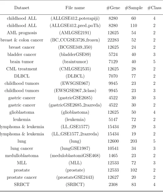
The microarray datasets1 _{utilized in this paper are listed in Table 1.}

320

There are 24 datasets, each of which is characterized by a very high feature number and low sample instance number. For each dataset, the data are normalized with respect to each feature; then, we generate a training set using the stratified bootstrap. Thus, the class distribution is maintained, and the samples that are not selected form the test set. Furthermore, the leave-325

one-out (LOO) methodology is employed for calculating the classification error.

1_{The utilized microarray datasets can be downloaded at}

http://www.biolab.si/

(15)

Table 1: Details of the Datasets

Dataset File name #Gene #Sample #Class

childhood ALL (ALLGSE412 poterapiji) 8280 60 4 childhood ALL (ALLGSE412 pred poTh) 8280 110 2

AML prognosis (AMLGSE2191) 12625 54 2

breast & colon cancer (BC CCGSE3726 frozen) 22283 52 2

breast cancer (BCGSE349 350) 12625 24 2

bladder cancer (bladderGSE89) 5724 40 3

brain tumor (braintumor) 7129 40 5

CML treatment (CMLGSE2535) 12625 28 2

DLBCL (DLBCL) 7070 77 2

childhood tumors (EWSGSE967) 9945 23 2

childhood tumors (EWSGSE967 3class) 9945 23 3

gastric cancer (gastricGSE2685) 4522 30 3

gastric cancer (gastricGSE2685 2razreda) 4522 30 2

glioblastoma (glioblastoma) 12625 50 4

leukemia (leukemia) 5147 72 2

lymphoma & leukemia (LL GSE1577) 15434 29 3

lymphoma & leukemia (LL GSE1577 2razreda) 15434 19 2

lung (lung) 12600 203 5

lung cancer (lungGSE1987) 10541 34 3

medulloblastoma (meduloblastomiGSE468) 1465 23 2

MLL (MLL) 12533 72 3

prostate (prostate) 12533 102 2

prostate cancer (prostateGSE2443) 12627 20 2

SRBCT (SRBCT) 2308 83 4

4.2. Utilized Algorithms and Parameter Settings

For comparison, four algorithms are utilized, as follows:

1. Cooperative coevolutionary generalized differential evolution 3 (CCGDE3) 330

(16)

2. Cooperative multiobjective differential evolution (CMODE) [28].

3. Multiobjective evolutionary algorithm based on decomposition (MOEA/D) [29].

4. Nondominated sorting genetic algorithm II (NSGA-II) [30]. 335

For a fair comparison, the population size of all algorithms is fixed to 120. In particular, for CCGDE3, there are two swarms, each of which has 60 individuals; for CMODE, there are three swarms for three objectives, with a size of 20 for each of them, and the size of the archive is 120.

The maximum number of FEs is 6×104_{. For each dataset, each MOEA}

340

runs 20 times.

In CCGDE3, DE [23, 24] is utilized, in whichF = 0.5 andCR = 1.0, and

the same settings are adopted in DE employed in MOEA/D. For CMODE, adaptive DE variants are utilized, and their parameter settings can be found in [31] and [25].

345

In NSGA-II, GA [9] is utilized, the distribution indices for crossover and

mutation are both 20, and their probabilities are 1.0 and _nDim1 , respectively.

For all the above algorithms, different encodings are tested, denoted as CCGDE3-FS, CCGDE3-FS-w, CMODE-FS, CMODE-FS-w, MOEA/D-FS, MOEA/D-FS-w, NSGA-II-FS and NSGA-II-FS-w. For the binary encod-350

ing, the feature adjustment in Section 3.3.3 is also added. Note that for

CCGDE3-FS, CMODE-FS, MOEA/D-FS and NSGA-II-FS, each variable is still encoded as a real value; thus, for the binary representation issue, a threshold (i.e., the mid-value) is utilized.

For the proposed algorithms, for DE, F follows the adaptive strategy in

355

JADE [25], while CR is fixed to 1.0 or adaptive as in JADE. The number of

variable groups is simply set to 5. For PM, its distribution index is 20, and

the probability is _nDim1 . Similar to MOEA/D, each individual corresponds

to a weight vector in the objective space, for which they have the same parameter settings.

360

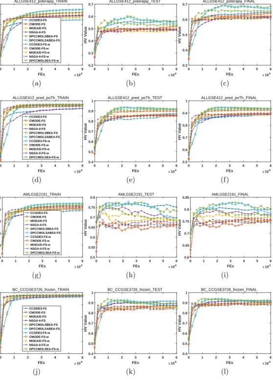
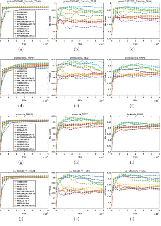
4.3. Analysis

In the following images (Fig. 1 to Fig. 24), there are three columns, corresponding to the training results, the test results and the final results. Specifically, for an obtained population, a feature subset is decoded from each individual. The classification error objective is calculated with respect 365

to the training set, the test set and the weighted sum of the former two, as follows:

(17)

f_EF IN AL = 0.368×f_ET RAIN + 0.632×f_ET EST (22)

where fF IN AL

E denotes the final classification error value, which depends on

fT RAIN

E and fET EST — classification errors on the training set and the test

set, respectively. Nevertheless, the remaining two objectives are only related 370

to the inherit property of the feature subset.

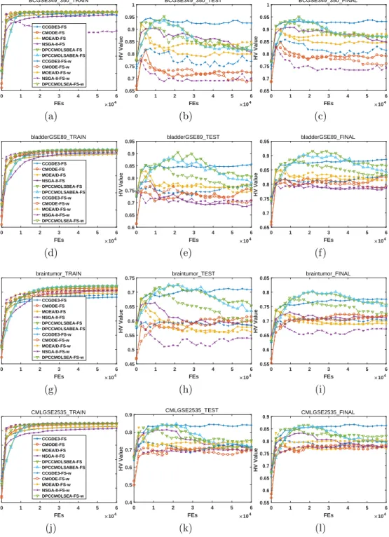
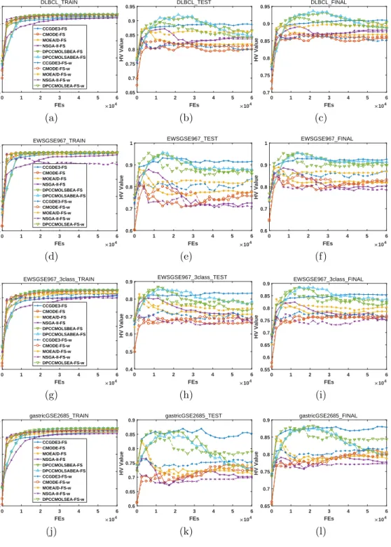
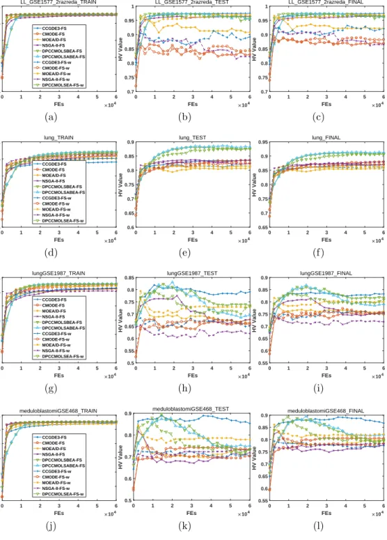
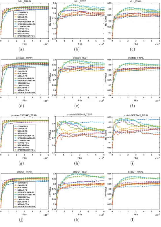
4.3.1. Hypervolume Indicator

In Figs. 1 to 6, we illustrate the hypervolume (HV) indicator [27] values, which can simultaneously measure the distribution and convergence of the obtained nondominated solutions during the evolution. For the reference 375

point in HV, because all objective values are not above 1, we set it as (1,1,1).

For the first column, we observe that the HV indicator values are monotonous-ly increasing, indicating that the qualities of the obtained nondominated

so-lutions are being ameliorated. Specifically, for the first approximately 104

FEs, the performance of all algorithms is improved rapidly; however, during 380

the following FEs, the improvement is minimal. For the second column, the HV indicator curves are not as monotonous because the classification error is derived based on the test set. At the beginning, the performance is improving quickly; then, however, for most datasets and algorithms, there are drops in the curves, indicating the occurrence of overfitting. In other words, although 385

the optimization performance on the training set is still good, the validation results on the test set deteriorate to some extent, and the situations become quite worse for some cases. Finally, by simultaneously considering the train-ing and testtrain-ing performance, the final optimization results are illustrated in the third column. Due to the nonmonotonic behavior of the results on the 390

test set, the final HV indicator values are also not monotonic during the evolutionary process.

Regarding the optimization performance of different algorithms, we have the following:

1. For the training results, the differences among various algorithms are 395

minimal. However, the proposed algorithms can always achieve the best results. For the two types of encodings, the weight-encoded ones converge faster than the binary-encoded ones. The ranking of other algorithms depends on the considered dataset.

(18)

2. For the test results, the performance varies. In most cases, overfitting 400

occurs. The common trend is that the indicator value increases rapidly to the maximum value within a very small number of FEs; then, over-fitting occurs, and the indicator value decreases or fluctuates. The only exception is the CCGDE3 algorithm, as its evolutionary curve only has slight fluctuations without a large drop, while the binary-encoded C-405

CGDE3 is much better than the weight-encoded one. However, with the view of the whole process, the peak HV indicator values are always obtained by the proposed algorithms.

3. For the final results, the proposed algorithms can generally obtain the peak HV indicator values.

410

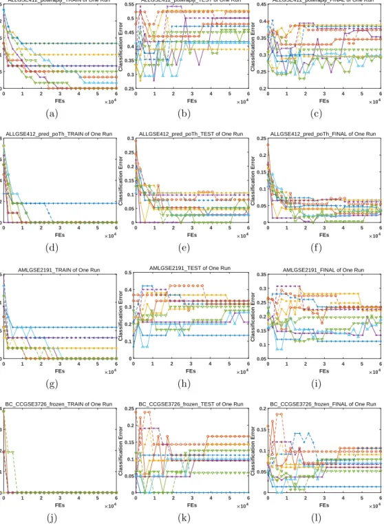
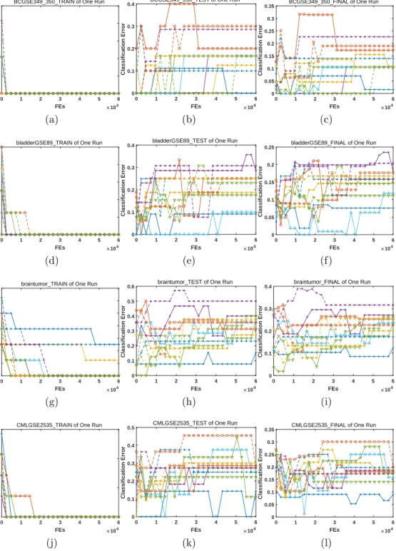
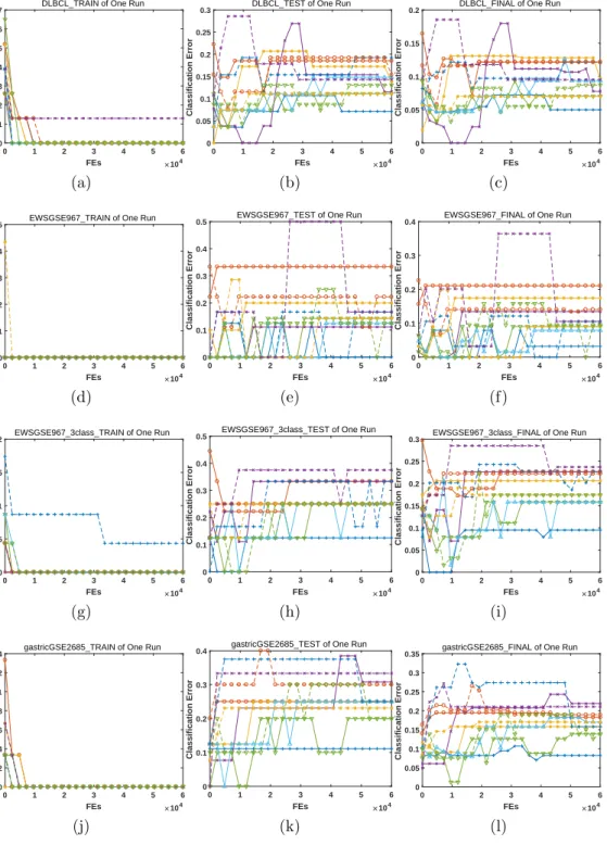
4.3.2. Classification Error

To better clarify the optimization results, we illustrate the lowest classi-fication errors during the evolutionary process of the run with median HV indicator value in Fig. 7 to Fig. 12. We can summarize the results as follows: 1. For the training data, in most cases, most algorithms can achieve zero 415

classification error. Especially, for 12 datasets of BC CCGSE3726 frozen,

BCGSE349 350, bladderGSE89, CMLGSE2535, EWSGSE967, gastricGSE2685, gastricGSE2685 2razreda, leukemia, LL GSE1577, LL GSE1577 2razreda, meduloblastomiGSE468 and prostateGSE2443, the classification errors remain at 0 almost during the whole evolutionary process. The dif-420

ference among all algorithms is the convergence issue, which is trivial. For the proposed algorithms, with respect to all datasets, there exists at least one algorithm that achieves zero classification error, and the same situation is also true for CMODE.

2. For the test data, the minimum classification error fluctuates violently 425

during evolution, which is more complex with respect to that on the training data; thus, we focus on the lowest value over the whole evolu-tion. For 20 out of 24datasets, zero classification error can be obtained; in particular, for the datasets of braintumor, MLL and prostate, only the proposed algorithms achieve zero classification error. On the con-430

trary, the classification errors obtained by CMODE are usually quite high, indicating the serious overfitting problem.

3. Comprehensively considering the training and test data, zero fication error indicates that the corresponding feature subset classi-fies all samples correctly in both the training data and the test data, 435

(19)

which is the expected result. For the following 13datasets of

ALL-GSE412 pred poTh, BC CCGSE3726 frozen, BCGSE349 350, bladderGSE89, DLBCL, EWSGSE967, EWSGSE967 3class, gastricGSE2685 2razreda,

LL GSE1577, LL GSE1577 2razreda, MLL, prostateGSE2443 and

S-RBCT, zero classification errors are observed. Specifically, for the

440

datasets of BC CCGSE3726 frozen and bladderGSE89, only the pro-posed algorithms can obtain zero classification error, while for all other datasets, the proposed algorithms are also generally not worse than their counterparts. And the binary-encoded ones are better than the weight-encoded one.

445

Corresponding to the above individuals with minimum classification er-rors, the feature numbers and feature redundancy are illustrated in the fol-lowing two subsections from Figs. 13 to 18 and Figs. 19 to 24, respectively.

4.3.3. Feature Number

For 15 datasets of ALLGSE412 pred poTh, BC CCGSE3726 frozen, BCGSE349 350, 450

CMLGSE2535, DLBCL, EWSGSE967, EWSGSE967 3class, gastricGSE2685, gastricGSE2685 2razreda, leukemia, LL GSE1577, LL GSE1577 2razreda, lung-GSE1987, meduloblastomiGSE468 and prostateGSE2443, illustrated in Figs.

13 to 18, all algorithms can generate a subset within 10 features (fN =

Nf

Nth F

=

10

50 = 0.2), except some special cases of CCGDE3. For the other datasets,

455

the feature number fluctuates along the evolution. With respect to the train-ing data and test data, however, in contrast to the status analyzed in the previous sections, the evolutionary curves share similar characteristics.

4.3.4. Feature Redundancy

For the feature redundancy objective, the evolutionary curves in Figs. 460

19 to 24 are characterized by undulations, which is subtle to comprehend. By formulating the feature redundancy as an objective, during the evolu-tion, it will lead the algorithm to form good-performing feature subsets with relatively few features with little redundancy.

4.3.5. Time Consumption

465

In Table 2, we list the average operating time for each algorithm with respect to each dataset. Additionally, the sum of time consumption over all datasets is listed in the second line from the bottom, and the speedup ratios are the values in parenthesis. With respect to the proposed algorithms, all

(20)

other MOEAs are at least one magnitude slower, except for the simple algo-470

rithm of CCGDE3-FS. For the proposed distributed algorithms, the number of utilized CPU cores is 60. Additionally, the speedup ratios with

respec-t respec-to respec-the mosrespec-t respec-time-consuming serial MOEA, CMODE, are 3.77E+ 01 and

4.91E+ 01, respectively, which are quite close to the ideal value of 60.

There-fore, we can conclude that the proposed algorithms are able to obtain better 475

(21)

0 1 2 3 4 5 6 FEs 104 0.4 0.5 0.6 0.7 0.8 0.9 1 HV Value ALLGSE412_poterapiji_TRAIN CCGDE3-FS CMODE-FS MOEA/D-FS NSGA-II-FS DPCCMOLSBEA-FS DPCCMOLSABEA-FS CCGDE3-FS-w CMODE-FS-w MOEA/D-FS-w NSGA-II-FS-w DPCCMOLSEA-FS-w (a) 0 1 2 3 4 5 6 FEs 104 0.2 0.3 0.4 0.5 0.6 0.7 HV Value ALLGSE412_poterapiji_TEST (b) 0 1 2 3 4 5 6 FEs 104 0.3 0.4 0.5 0.6 0.7 HV Value ALLGSE412_poterapiji_FINAL (c) 0 1 2 3 4 5 6 FEs 104 0.6 0.7 0.8 0.9 1 HV Value ALLGSE412_pred_poTh_TRAIN CCGDE3-FS CMODE-FS MOEA/D-FS NSGA-II-FS DPCCMOLSBEA-FS DPCCMOLSABEA-FS CCGDE3-FS-w CMODE-FS-w MOEA/D-FS-w NSGA-II-FS-w DPCCMOLSEA-FS-w (d) 0 1 2 3 4 5 6 FEs 104 0.4 0.5 0.6 0.7 0.8 0.9 1 HV Value ALLGSE412_pred_poTh_TEST (e) 0 1 2 3 4 5 6 FEs 104 0.5 0.6 0.7 0.8 0.9 1 HV Value ALLGSE412_pred_poTh_FINAL (f) 0 1 2 3 4 5 6 FEs 104 0.75 0.8 0.85 0.9 0.95 1 HV Value AMLGSE2191_TRAIN CCGDE3-FS CMODE-FS MOEA/D-FS NSGA-II-FS DPCCMOLSBEA-FS DPCCMOLSABEA-FS CCGDE3-FS-w CMODE-FS-w MOEA/D-FS-w NSGA-II-FS-w DPCCMOLSEA-FS-w (g) 0 1 2 3 4 5 6 FEs 104 0.5 0.55 0.6 0.65 0.7 0.75 0.8 HV Value AMLGSE2191_TEST (h) 0 1 2 3 4 5 6 FEs 104 0.6 0.65 0.7 0.75 0.8 0.85 HV Value AMLGSE2191_FINAL (i) 0 1 2 3 4 5 6 FEs 104 0.5 0.6 0.7 0.8 0.9 1 HV Value BC_CCGSE3726_frozen_TRAIN CCGDE3-FS CMODE-FS MOEA/D-FS NSGA-II-FS DPCCMOLSBEA-FS DPCCMOLSABEA-FS CCGDE3-FS-w CMODE-FS-w MOEA/D-FS-w NSGA-II-FS-w DPCCMOLSEA-FS-w (j) 0 1 2 3 4 5 6 FEs 104 0.4 0.5 0.6 0.7 0.8 0.9 1 HV Value BC_CCGSE3726_frozen_TEST (k) 0 1 2 3 4 5 6 FEs 104 0.4 0.5 0.6 0.7 0.8 0.9 1 HV Value BC_CCGSE3726_frozen_FINAL (l)

(22)

0 1 2 3 4 5 6 FEs 104 0.75 0.8 0.85 0.9 0.95 1 HV Value BCGSE349_350_TRAIN CCGDE3-FS CMODE-FS MOEA/D-FS NSGA-II-FS DPCCMOLSBEA-FS DPCCMOLSABEA-FS CCGDE3-FS-w CMODE-FS-w MOEA/D-FS-w NSGA-II-FS-w DPCCMOLSEA-FS-w (a) 0 1 2 3 4 5 6 FEs 104 0.65 0.7 0.75 0.8 0.85 0.9 0.95 1 HV Value BCGSE349_350_TEST (b) 0 1 2 3 4 5 6 FEs 104 0.65 0.7 0.75 0.8 0.85 0.9 0.95 1 HV Value BCGSE349_350_FINAL (c) 0 1 2 3 4 5 6 FEs 104 0.75 0.8 0.85 0.9 0.95 1 HV Value bladderGSE89_TRAIN CCGDE3-FS CMODE-FS MOEA/D-FS NSGA-II-FS DPCCMOLSBEA-FS DPCCMOLSABEA-FS CCGDE3-FS-w CMODE-FS-w MOEA/D-FS-w NSGA-II-FS-w DPCCMOLSEA-FS-w (d) 0 1 2 3 4 5 6 FEs 104 0.6 0.65 0.7 0.75 0.8 0.85 0.9 0.95 HV Value bladderGSE89_TEST (e) 0 1 2 3 4 5 6 FEs 104 0.65 0.7 0.75 0.8 0.85 0.9 0.95 HV Value bladderGSE89_FINAL (f) 0 1 2 3 4 5 6 FEs 104 0.7 0.75 0.8 0.85 0.9 0.95 1 HV Value braintumor_TRAIN CCGDE3-FS CMODE-FS MOEA/D-FS NSGA-II-FS DPCCMOLSBEA-FS DPCCMOLSABEA-FS CCGDE3-FS-w CMODE-FS-w MOEA/D-FS-w NSGA-II-FS-w DPCCMOLSEA-FS-w (g) 0 1 2 3 4 5 6 FEs 104 0.45 0.5 0.55 0.6 0.65 0.7 0.75 HV Value braintumor_TEST (h) 0 1 2 3 4 5 6 FEs 104 0.55 0.6 0.65 0.7 0.75 0.8 0.85 HV Value braintumor_FINAL (i) 0 1 2 3 4 5 6 FEs 104 0.7 0.75 0.8 0.85 0.9 0.95 1 HV Value CMLGSE2535_TRAIN CCGDE3-FS CMODE-FS MOEA/D-FS NSGA-II-FS DPCCMOLSBEA-FS DPCCMOLSABEA-FS CCGDE3-FS-w CMODE-FS-w MOEA/D-FS-w NSGA-II-FS-w DPCCMOLSEA-FS-w (j) 0 1 2 3 4 5 6 FEs 104 0.4 0.5 0.6 0.7 0.8 0.9 HV Value CMLGSE2535_TEST (k) 0 1 2 3 4 5 6 FEs 104 0.55 0.6 0.65 0.7 0.75 0.8 0.85 0.9 HV Value CMLGSE2535_FINAL (l)

(23)

0 1 2 3 4 5 6 FEs 104 0.75 0.8 0.85 0.9 0.95 1 HV Value DLBCL_TRAIN CCGDE3-FS CMODE-FS MOEA/D-FS NSGA-II-FS DPCCMOLSBEA-FS DPCCMOLSABEA-FS CCGDE3-FS-w CMODE-FS-w MOEA/D-FS-w NSGA-II-FS-w DPCCMOLSEA-FS-w (a) 0 1 2 3 4 5 6 FEs 104 0.65 0.7 0.75 0.8 0.85 0.9 0.95 HV Value DLBCL_TEST (b) 0 1 2 3 4 5 6 FEs 104 0.7 0.75 0.8 0.85 0.9 0.95 HV Value DLBCL_FINAL (c) 0 1 2 3 4 5 6 FEs 104 0.75 0.8 0.85 0.9 0.95 1 HV Value EWSGSE967_TRAIN CCGDE3-FS CMODE-FS MOEA/D-FS NSGA-II-FS DPCCMOLSBEA-FS DPCCMOLSABEA-FS CCGDE3-FS-w CMODE-FS-w MOEA/D-FS-w NSGA-II-FS-w DPCCMOLSEA-FS-w (d) 0 1 2 3 4 5 6 FEs 104 0.6 0.7 0.8 0.9 1 HV Value EWSGSE967_TEST (e) 0 1 2 3 4 5 6 FEs 104 0.6 0.7 0.8 0.9 1 HV Value EWSGSE967_FINAL (f) 0 1 2 3 4 5 6 FEs 104 0.7 0.75 0.8 0.85 0.9 0.95 1 HV Value EWSGSE967_3class_TRAIN CCGDE3-FS CMODE-FS MOEA/D-FS NSGA-II-FS DPCCMOLSBEA-FS DPCCMOLSABEA-FS CCGDE3-FS-w CMODE-FS-w MOEA/D-FS-w NSGA-II-FS-w DPCCMOLSEA-FS-w (g) 0 1 2 3 4 5 6 FEs 104 0.4 0.5 0.6 0.7 0.8 0.9 HV Value EWSGSE967_3class_TEST (h) 0 1 2 3 4 5 6 FEs 104 0.55 0.6 0.65 0.7 0.75 0.8 0.85 0.9 HV Value EWSGSE967_3class_FINAL (i) 0 1 2 3 4 5 6 FEs 104 0.75 0.8 0.85 0.9 0.95 1 HV Value gastricGSE2685_TRAIN CCGDE3-FS CMODE-FS MOEA/D-FS NSGA-II-FS DPCCMOLSBEA-FS DPCCMOLSABEA-FS CCGDE3-FS-w CMODE-FS-w MOEA/D-FS-w NSGA-II-FS-w DPCCMOLSEA-FS-w (j) 0 1 2 3 4 5 6 FEs 104 0.6 0.65 0.7 0.75 0.8 0.85 0.9 HV Value gastricGSE2685_TEST (k) 0 1 2 3 4 5 6 FEs 104 0.65 0.7 0.75 0.8 0.85 0.9 HV Value gastricGSE2685_FINAL (l)

(24)

0 1 2 3 4 5 6 FEs 104 0.8 0.85 0.9 0.95 1 HV Value gastricGSE2685_2razreda_TRAIN CCGDE3-FS CMODE-FS MOEA/D-FS NSGA-II-FS DPCCMOLSBEA-FS DPCCMOLSABEA-FS CCGDE3-FS-w CMODE-FS-w MOEA/D-FS-w NSGA-II-FS-w DPCCMOLSEA-FS-w (a) 0 1 2 3 4 5 6 FEs 104 0.75 0.8 0.85 0.9 0.95 1 HV Value gastricGSE2685_2razreda_TEST (b) 0 1 2 3 4 5 6 FEs 104 0.75 0.8 0.85 0.9 0.95 1 HV Value gastricGSE2685_2razreda_FINAL (c) 0 1 2 3 4 5 6 FEs 104 0.7 0.75 0.8 0.85 0.9 0.95 1 HV Value glioblastoma_TRAIN CCGDE3-FS CMODE-FS MOEA/D-FS NSGA-II-FS DPCCMOLSBEA-FS DPCCMOLSABEA-FS CCGDE3-FS-w CMODE-FS-w MOEA/D-FS-w NSGA-II-FS-w DPCCMOLSEA-FS-w (d) 0 1 2 3 4 5 6 FEs 104 0.45 0.5 0.55 0.6 0.65 0.7 0.75 HV Value glioblastoma_TEST (e) 0 1 2 3 4 5 6 FEs 104 0.55 0.6 0.65 0.7 0.75 0.8 0.85 HV Value glioblastoma_FINAL (f) 0 1 2 3 4 5 6 FEs 104 0.8 0.85 0.9 0.95 1 HV Value leukemia_TRAIN CCGDE3-FS CMODE-FS MOEA/D-FS NSGA-II-FS DPCCMOLSBEA-FS DPCCMOLSABEA-FS CCGDE3-FS-w CMODE-FS-w MOEA/D-FS-w NSGA-II-FS-w DPCCMOLSEA-FS-w (g) 0 1 2 3 4 5 6 FEs 104 0.65 0.7 0.75 0.8 0.85 0.9 0.95 HV Value leukemia_TEST (h) 0 1 2 3 4 5 6 FEs 104 0.7 0.75 0.8 0.85 0.9 0.95 1 HV Value leukemia_FINAL (i) 0 1 2 3 4 5 6 FEs 104 0.75 0.8 0.85 0.9 0.95 1 HV Value LL_GSE1577_TRAIN CCGDE3-FS CMODE-FS MOEA/D-FS NSGA-II-FS DPCCMOLSBEA-FS DPCCMOLSABEA-FS CCGDE3-FS-w CMODE-FS-w MOEA/D-FS-w NSGA-II-FS-w DPCCMOLSEA-FS-w (j) 0 1 2 3 4 5 6 FEs 104 0.6 0.65 0.7 0.75 0.8 0.85 0.9 0.95 HV Value LL_GSE1577_TEST (k) 0 1 2 3 4 5 6 FEs 104 0.65 0.7 0.75 0.8 0.85 0.9 0.95 HV Value LL_GSE1577_FINAL (l)

(25)

0 1 2 3 4 5 6 FEs 104 0.75 0.8 0.85 0.9 0.95 1 HV Value LL_GSE1577_2razreda_TRAIN CCGDE3-FS CMODE-FS MOEA/D-FS NSGA-II-FS DPCCMOLSBEA-FS DPCCMOLSABEA-FS CCGDE3-FS-w CMODE-FS-w MOEA/D-FS-w NSGA-II-FS-w DPCCMOLSEA-FS-w (a) 0 1 2 3 4 5 6 FEs 104 0.7 0.75 0.8 0.85 0.9 0.95 1 HV Value LL_GSE1577_2razreda_TEST (b) 0 1 2 3 4 5 6 FEs 104 0.7 0.75 0.8 0.85 0.9 0.95 1 HV Value LL_GSE1577_2razreda_FINAL (c) 0 1 2 3 4 5 6 FEs 104 0.75 0.8 0.85 0.9 0.95 1 HV Value lung_TRAIN CCGDE3-FS CMODE-FS MOEA/D-FS NSGA-II-FS DPCCMOLSBEA-FS DPCCMOLSABEA-FS CCGDE3-FS-w CMODE-FS-w MOEA/D-FS-w NSGA-II-FS-w DPCCMOLSEA-FS-w (d) 0 1 2 3 4 5 6 FEs 104 0.6 0.65 0.7 0.75 0.8 0.85 0.9 HV Value lung_TEST (e) 0 1 2 3 4 5 6 FEs 104 0.65 0.7 0.75 0.8 0.85 0.9 0.95 HV Value lung_FINAL (f) 0 1 2 3 4 5 6 FEs 104 0.7 0.75 0.8 0.85 0.9 0.95 1 HV Value lungGSE1987_TRAIN CCGDE3-FS CMODE-FS MOEA/D-FS NSGA-II-FS DPCCMOLSBEA-FS DPCCMOLSABEA-FS CCGDE3-FS-w CMODE-FS-w MOEA/D-FS-w NSGA-II-FS-w DPCCMOLSEA-FS-w (g) 0 1 2 3 4 5 6 FEs 104 0.5 0.55 0.6 0.65 0.7 0.75 0.8 0.85 HV Value lungGSE1987_TEST (h) 0 1 2 3 4 5 6 FEs 104 0.55 0.6 0.65 0.7 0.75 0.8 0.85 0.9 HV Value lungGSE1987_FINAL (i) 0 1 2 3 4 5 6 FEs 104 0.7 0.75 0.8 0.85 0.9 0.95 1 HV Value meduloblastomiGSE468_TRAIN CCGDE3-FS CMODE-FS MOEA/D-FS NSGA-II-FS DPCCMOLSBEA-FS DPCCMOLSABEA-FS CCGDE3-FS-w CMODE-FS-w MOEA/D-FS-w NSGA-II-FS-w DPCCMOLSEA-FS-w (j) 0 1 2 3 4 5 6 FEs 104 0.5 0.6 0.7 0.8 0.9 HV Value meduloblastomiGSE468_TEST (k) 0 1 2 3 4 5 6 FEs 104 0.55 0.6 0.65 0.7 0.75 0.8 0.85 0.9 HV Value meduloblastomiGSE468_FINAL (l)

(26)

0 1 2 3 4 5 6 FEs 104 0.75 0.8 0.85 0.9 0.95 1 HV Value MLL_TRAIN CCGDE3-FS CMODE-FS MOEA/D-FS NSGA-II-FS DPCCMOLSBEA-FS DPCCMOLSABEA-FS CCGDE3-FS-w CMODE-FS-w MOEA/D-FS-w NSGA-II-FS-w DPCCMOLSEA-FS-w (a) 0 1 2 3 4 5 6 FEs 104 0.55 0.6 0.65 0.7 0.75 0.8 0.85 0.9 HV Value MLL_TEST (b) 0 1 2 3 4 5 6 FEs 104 0.65 0.7 0.75 0.8 0.85 0.9 0.95 HV Value MLL_FINAL (c) 0 1 2 3 4 5 6 FEs 104 0.7 0.75 0.8 0.85 0.9 0.95 1 HV Value prostate_TRAIN CCGDE3-FS CMODE-FS MOEA/D-FS NSGA-II-FS DPCCMOLSBEA-FS DPCCMOLSABEA-FS CCGDE3-FS-w CMODE-FS-w MOEA/D-FS-w NSGA-II-FS-w DPCCMOLSEA-FS-w (d) 0 1 2 3 4 5 6 FEs 104 0.55 0.6 0.65 0.7 0.75 0.8 0.85 0.9 HV Value prostate_TEST (e) 0 1 2 3 4 5 6 FEs 104 0.6 0.65 0.7 0.75 0.8 0.85 0.9 0.95 HV Value prostate_FINAL (f) 0 1 2 3 4 5 6 FEs 104 0.75 0.8 0.85 0.9 0.95 1 HV Value prostateGSE2443_TRAIN CCGDE3-FS CMODE-FS MOEA/D-FS NSGA-II-FS DPCCMOLSBEA-FS DPCCMOLSABEA-FS CCGDE3-FS-w CMODE-FS-w MOEA/D-FS-w NSGA-II-FS-w DPCCMOLSEA-FS-w (g) 0 1 2 3 4 5 6 FEs 104 0.5 0.6 0.7 0.8 0.9 1 HV Value prostateGSE2443_TEST (h) 0 1 2 3 4 5 6 FEs 104 0.6 0.65 0.7 0.75 0.8 0.85 0.9 0.95 HV Value prostateGSE2443_FINAL (i) 0 1 2 3 4 5 6 FEs 104 0.75 0.8 0.85 0.9 0.95 1 HV Value SRBCT_TRAIN CCGDE3-FS CMODE-FS MOEA/D-FS NSGA-II-FS DPCCMOLSBEA-FS DPCCMOLSABEA-FS CCGDE3-FS-w CMODE-FS-w MOEA/D-FS-w NSGA-II-FS-w DPCCMOLSEA-FS-w (j) 0 1 2 3 4 5 6 FEs 104 0.55 0.6 0.65 0.7 0.75 0.8 0.85 0.9 HV Value SRBCT_TEST (k) 0 1 2 3 4 5 6 FEs 104 0.6 0.65 0.7 0.75 0.8 0.85 0.9 0.95 HV Value SRBCT_FINAL (l)

(27)

0 1 2 3 4 5 6 FEs 104 0 0.05 0.1 0.15 0.2 0.25 Classification Error

ALLGSE412_poterapiji_TRAIN of One Run

(a) 0 1 2 3 4 5 6 FEs 104 0.25 0.3 0.35 0.4 0.45 0.5 0.55 Classification Error

ALLGSE412_poterapiji_TEST of One Run

(b) 0 1 2 3 4 5 6 FEs 104 0.2 0.25 0.3 0.35 0.4 0.45 Classification Error

ALLGSE412_poterapiji_FINAL of One Run

(c) 0 1 2 3 4 5 6 FEs 104 0 0.02 0.04 0.06 0.08 Classification Error

ALLGSE412_pred_poTh_TRAIN of One Run

(d) 0 1 2 3 4 5 6 FEs 104 0 0.05 0.1 0.15 0.2 0.25 0.3 Classification Error

ALLGSE412_pred_poTh_TEST of One Run

(e) 0 1 2 3 4 5 6 FEs 104 0 0.05 0.1 0.15 0.2 0.25 Classification Error

ALLGSE412_pred_poTh_FINAL of One Run

(f) 0 1 2 3 4 5 6 FEs 104 0 0.05 0.1 0.15 Classification Error

AMLGSE2191_TRAIN of One Run

(g) 0 1 2 3 4 5 6 FEs 104 0 0.1 0.2 0.3 0.4 0.5 Classification Error

AMLGSE2191_TEST of One Run

(h) 0 1 2 3 4 5 6 FEs 104 0.05 0.1 0.15 0.2 0.25 0.3 0.35 Classification Error

AMLGSE2191_FINAL of One Run

(i) 0 1 2 3 4 5 6 FEs 104 0 0.01 0.02 0.03 0.04 Classification Error

BC_CCGSE3726_frozen_TRAIN of One Run

(j) 0 1 2 3 4 5 6 FEs 104 0 0.05 0.1 0.15 0.2 0.25 Classification Error

BC_CCGSE3726_frozen_TEST of One Run

(k) 0 1 2 3 4 5 6 FEs 104 0 0.05 0.1 0.15 0.2 Classification Error

BC_CCGSE3726_frozen_FINAL of One Run

(l)

(28)

BCGSE349_350_TRAIN of One Run

(a) 0 1 2 3 4 5 6 FEs 104 0 0.1 0.2 0.3 0.4 Classification Error

BCGSE349_350_TEST of One Run

(b) 0 1 2 3 4 5 6 FEs 104 0 0.05 0.1 0.15 0.2 0.25 0.3 0.35 Classification Error

BCGSE349_350_FINAL of One Run

(c) 0 1 2 3 4 5 6 FEs 104 0 0.02 0.04 0.06 0.08 0.1 Classification Error

bladderGSE89_TRAIN of One Run

(d) 0 1 2 3 4 5 6 FEs 104 0 0.1 0.2 0.3 0.4 Classification Error

bladderGSE89_TEST of One Run

bladderGSE89_FINAL of One Run

(f) 0 1 2 3 4 5 6 FEs 104 0 0.02 0.04 0.06 0.08 0.1 0.12 0.14 Classification Error

braintumor_TRAIN of One Run

(g) 0 1 2 3 4 5 6 FEs 104 0 0.1 0.2 0.3 0.4 0.5 0.6 Classification Error

braintumor_TEST of One Run

(h) 0 1 2 3 4 5 6 FEs 104 0 0.1 0.2 0.3 0.4 Classification Error

braintumor_FINAL of One Run

(i) 0 1 2 3 4 5 6 FEs 104 0 0.05 0.1 0.15 Classification Error

CMLGSE2535_TRAIN of One Run

CMLGSE2535_TEST of One Run

(k) 0 1 2 3 4 5 6 FEs 104 0 0.05 0.1 0.15 0.2 0.25 0.3 0.35 Classification Error

CMLGSE2535_FINAL of One Run

(l)

(29)

0 1 2 3 4 5 6 FEs 104 0 0.01 0.02 0.03 0.04 0.05 0.06 0.07 Classification Error

DLBCL_TRAIN of One Run

(a) 0 1 2 3 4 5 6 FEs 104 0 0.05 0.1 0.15 0.2 0.25 0.3 Classification Error

DLBCL_TEST of One Run

(b) 0 1 2 3 4 5 6 FEs 104 0 0.05 0.1 0.15 0.2 Classification Error

DLBCL_FINAL of One Run

EWSGSE967_TRAIN of One Run

(d) 0 1 2 3 4 5 6 FEs 104 0 0.1 0.2 0.3 0.4 0.5 Classification Error

EWSGSE967_TEST of One Run

(e) 0 1 2 3 4 5 6 FEs 104 0 0.1 0.2 0.3 0.4 Classification Error

EWSGSE967_FINAL of One Run

(f) 0 1 2 3 4 5 6 FEs 104 0 0.05 0.1 0.15 0.2 Classification Error

EWSGSE967_3class_TRAIN of One Run

EWSGSE967_3class_TEST of One Run

(h) 0 1 2 3 4 5 6 FEs 104 0 0.05 0.1 0.15 0.2 0.25 0.3 Classification Error

EWSGSE967_3class_FINAL of One Run

(i) 0 1 2 3 4 5 6 FEs 104 0 0.02 0.04 0.06 0.08 0.1 0.12 0.14 Classification Error

gastricGSE2685_TRAIN of One Run

(j) 0 1 2 3 4 5 6 FEs 104 0 0.1 0.2 0.3 0.4 Classification Error

gastricGSE2685_TEST of One Run

gastricGSE2685_FINAL of One Run

(l)

(30)

0 1 2 3 4 5 6 FEs 104 -1 -0.5 0 0.5 1 Classification Error

gastricGSE2685_2razreda_TRAIN of One Run

gastricGSE2685_2razreda_TEST of One Run

gastricGSE2685_2razreda_FINAL of One Run

(c) 0 1 2 3 4 5 6 FEs 104 0 0.02 0.04 0.06 0.08 0.1 0.12 Classification Error

glioblastoma_TRAIN of One Run

(d) 0 1 2 3 4 5 6 FEs 104 0.1 0.2 0.3 0.4 0.5 Classification Error

glioblastoma_TEST of One Run

(e) 0 1 2 3 4 5 6 FEs 104 0.05 0.1 0.15 0.2 0.25 0.3 0.35 Classification Error

glioblastoma_FINAL of One Run

(f) 0 1 2 3 4 5 6 FEs 104 0 0.01 0.02 0.03 0.04 0.05 0.06 Classification Error

leukemia_TRAIN of One Run

leukemia_TEST of One Run

(h) 0 1 2 3 4 5 6 FEs 104 0 0.05 0.1 0.15 Classification Error

leukemia_FINAL of One Run

(i) 0 1 2 3 4 5 6 FEs 104 0 0.005 0.01 0.015 0.02 0.025 0.03 0.035 Classification Error

LL_GSE1577_TRAIN of One Run

LL_GSE1577_TEST of One Run

(k) 0 1 2 3 4 5 6 FEs 104 0 0.05 0.1 0.15 0.2 0.25 0.3 Classification Error

LL_GSE1577_FINAL of One Run

(l)

(31)

0 1 2 3 4 5 6 FEs 104 -1 -0.5 0 0.5 1 Classification Error

LL_GSE1577_2razreda_TRAIN of One Run

(a) 0 1 2 3 4 5 6 FEs 104 0 0.05 0.1 0.15 0.2 Classification Error

LL_GSE1577_2razreda_TEST of One Run

LL_GSE1577_2razreda_FINAL of One Run

lung_TRAIN of One Run

(d) 0 1 2 3 4 5 6 FEs 104 0.04 0.06 0.08 0.1 0.12 0.14 0.16 0.18 Classification Error

lung_TEST of One Run

(e) 0 1 2 3 4 5 6 FEs 104 0.02 0.04 0.06 0.08 0.1 0.12 0.14 Classification Error

lung_FINAL of One Run

lungGSE1987_TRAIN of One Run

lungGSE1987_TEST of One Run

(h) 0 1 2 3 4 5 6 FEs 104 0 0.05 0.1 0.15 0.2 0.25 0.3 Classification Error

lungGSE1987_FINAL of One Run

(i) 0 1 2 3 4 5 6 FEs 104 0 0.02 0.04 0.06 0.08 0.1 Classification Error

meduloblastomiGSE468_TRAIN of One Run

meduloblastomiGSE468_TEST of One Run

meduloblastomiGSE468_FINAL of One Run

(l)

(32)

MLL_TRAIN of One Run

MLL_TEST of One Run

MLL_FINAL of One Run

(c) 0 1 2 3 4 5 6 FEs 104 0 0.02 0.04 0.06 0.08 Classification Error

prostate_TRAIN of One Run

(d) 0 1 2 3 4 5 6 FEs 104 0 0.05 0.1 0.15 0.2 0.25 0.3 0.35 Classification Error

prostate_TEST of One Run

prostate_FINAL of One Run

prostateGSE2443_TRAIN of One Run

(g) 0 1 2 3 4 5 6 FEs 104 0 0.05 0.1 0.15 0.2 0.25 0.3 0.35 Classification Error

prostateGSE2443_TEST of One Run

(h) 0 1 2 3 4 5 6 FEs 104 0 0.05 0.1 0.15 0.2 0.25 Classification Error

prostateGSE2443_FINAL of One Run

(i) 0 1 2 3 4 5 6 FEs 104 0 0.02 0.04 0.06 0.08 0.1 0.12 Classification Error

SRBCT_TRAIN of One Run

(j) 0 1 2 3 4 5 6 FEs 104 0 0.05 0.1 0.15 0.2 0.25 0.3 0.35 Classification Error

SRBCT_TEST of One Run

(k) 0 1 2 3 4 5 6 FEs 104 0 0.05 0.1 0.15 0.2 0.25 Classification Error

SRBCT_FINAL of One Run

(l)