Modelling the tone reproduction characteristics of digital printers using continuous tone model

Rochester Institute of Technology

RIT Scholar Works

Theses

Thesis/Dissertation Collections

8-1-2003

Modelling the tone reproduction characteristics of

digital printers using continuous tone model

Prashant Mehta

Follow this and additional works at:

http://scholarworks.rit.edu/theses

This Thesis is brought to you for free and open access by the Thesis/Dissertation Collections at RIT Scholar Works. It has been accepted for inclusion

in Theses by an authorized administrator of RIT Scholar Works. For more information, please contact

[email protected]

.

Recommended Citation

Modelling The Tone Reproduction Characteristics of Digital

Printers Using Continuous Tone Model

By

Prashant P. Mehta

B.E. (Chemical) L. D. College of Engineering, Ahmedabad, India

(1997)

A thesis submitted in partial fulfillment of the

requirements for the degree of Master of Science

in the Chester F. Carlson Center for Imaging Science

of the College of Science

Rochester Institute of Technology

August 2003

Signature of the Author

_

CHESTER F. CARLSON

CENTER FOR IMAGING SCIENCE

COLLEGE OF SCIENCE

ROCHESTER INSTITUTE OF TECHNOLOGY

ROCHESTER, NEW YORK

CERTIFICATE OF APPROVAL

M.S. DEGREE THESIS

The M.S. Degree Thesis of Prashant P. Mehta

has been examined and approved by the

thesis committee as satisfactory for the

thesis requirement for the

Master of Science degree

Dr. Jonathan S. Arney, Thesis Advisor

Dr. Peter Anderson

Dr. Jeffery Pelz

THESIS RELEASE

PERMISSION

ROCHESTER INSTITUTE OF TECHNOLOGY

COLLEGE OF SCIENCE

CHESTER F. CARLSON

CENTER FOR IMAGING SCIENCE

Title

of

Thesis:

Modelling

The Tone

Reproduction

Characteristics

of

Digital

Printers

Using

Continuous Tone

Model

I,

Prashant

P.

Mehta,

hereby

grant

permission

to the

Wallace

Memorial

Library

of

R.I.T.

to

reproduce

my

thesis

in

whole or

in

Modelling

The Tone

Reproduction Characteristics

of

Digital

Printers

Using

Continuous

Tone Model

by

Prashant P. Mehta

Submitted

to the

Chester F. Carlson Center

for

Imaging

Science College

of

Science in

partial

fulfillment

of

the

requirements

for

the

Master

of

Science Degree

at

the

Rochester Institute

of

Technology

ABSTRACT

Traditional

halftone

models

have been

used

to

characterize

the

tone

reproduction

characteristics

of

digital

printers.

These

models

can

be

corrected

to

incorporate

system parameters

like light

scattering,

softer

dot

edge etc.

This

thesis

work explores

the

possibility

of

applying

the

modified

continuous

tone

model

to

characterize

the

tone

reproduction

of

high

addressibility

printers.

Both

the

continuous

tone

model and

the

modified

halftone

model will

be

compared

for

how

well

they

characterize

the tone

ACKNOWLEDGEMENTS

I

wish

to

acknowledge

wonderful and patient support of

my

thesis

advisor

Dr. Jonathan

Arney. In

the

years

that

I have

spent

in Dr. Arney's

guidance,

I

have

come

to

respect

his

"healthy

skepticism"

approach

to

research.

Dr.

Peter Anderson

has been helpful in providing different

prints

that

are

used

in

this thesis

for

analysis.

I

am also

thankful

to

Dr. Pelz for

all

his

help

on

this

project.

Had it

not

been for

patience and persistence of

my

wife

Vasanthi

and

my

parents

Pradeep

and

Mallika,

I may have

not

been

able

to

bring

this

project

to

a completion.

I

also wish

to thank

my friends Kate Johnson

and

Joan

Ashley

for

their

support.

This

research

has been funded

by

Hewlett-Packard

and

I

wish

to

extend

my

thanks

for

their

financial

support.

And,

the

work was

conducted

in

-

Contents

-List

of

figures

List

of

tables

1.

Introduction

2.

Background Literature Review

2.1.

Electrophotographic Printers

2.2.

Halftoning

2.2. 1

.

The

origins of

halftoning

process

2.2.2.

Halftones for digital

printers

2.2.3.

Clustered dot

2.2.4.

Dispersed dot

2.2.5.

Noise

power

in halftone images

2.2.6.

Floy

d S

teinberg

halftone

2.3.

Literature

review of

tone

reproduction

behavior

of

halftones

2.3.1.

Murray-Davies

equation

2.3.2.

The Yule-Nielsen

equation

2.3.3.

Recent

developments in

mechanistic

halftone modeling

2.3.4.

The probability

model

2.3.5.

Modeling

P00

for Different Halftone Systems

3.

Behavior

of

halftones

printedon

EP

printers

3.1.

Tone behavior

of

halftones in

histograms

3.2.

Observation

of printed

images

atmicroscopic

level

and point spread

function

ofnon-coatedpaper

4.

Continuous

Tone Model

4. 1

.

Beer-Lambert Transmittance

4.2.

Beer-Lambert Reflectance

4.3.

Applying

the

Beer-Lambert Model

to

a

Halftone

4.4.

Kubelka-Munk Model

4.5.

Spatial

Efficiency

Function

4.5. 1

.

An

Empirical Function

4.5.2.

The Beer-Lambert Model Modified

with

the

Spatial Absorption Function

4.5.3.

The

Kubelka-Munk Model Modified

with

the

Spatial Absorption Function

4.6.

Relating

the

Printing

Resolution

to

Spatial

Efficiency

Function

4.6.1.

The

"A"

Parameter

4.7.

Conclusion

and

Recommendations

5.

Conclusions

Appendix

A:

Experimental

procedures

A.l

Densitometry

-

List

of

figures

-Chapter

1

Figure 1.1: Halftone Image

Chapter

2

Figure 2.1: Mechanism

of electrophotographic printers

Figure 2.2: Copperplate engraving

of

Johann

Gutenberg by

Andre

Thevet, Paris, 1584,

from

the

RIT

Cary

Collection.

Detail

on

the

right

illustrates

spatial modulation

Figure 2.3: Matrix representing

the

printer

addressability

Figure 2.4: Example

of

producing

clustered

dot using individual

printer spots

Figure

2.5:

Gray

wedge printed with

(a)

Clustered dot

(b)

Dispersed

dot

Figure

2.6: Examples

of

Floyd-Steinberg

Halftones

Figure

2.7: Reflectance

vs

Dot

area

fraction,

individual

points are

the

measured

data

and continuous

line

represents

Murray

Davis

Equation

Figure

2.8: R

vs.

F

modeled

by

Yule-Nielsen

equation

for

n=l and

Chapter 3:

Figure

3.1: Image

and

histogram

of an

ideal halftone

(R=0.75)

Figure 3.2: Image

and

histogram

of an

ideal halftone

system

(R

=

0.5)

Figure 3.3: Histograms

of

ideal

continuous

tone

system,

at

R=0.5

and

R

=

0.75

Figure 3.4: Histogram

of

Floyd-Steinberg

halftone

(Fn=0.1)

printed on

300 dpi EP

printer

Figure 3.5: Histogram

of

Floyd-Steinberg

halftone (Fn

=0.3)

printed on

300 dpi EP

printer

Figure 3.6: Histogram

of a

Floyd-Steinberg

halftone

printed on a

600

dpi

printer,

Fn

=0.0625

Figure 3.7: Histogram

of a

Floyd-Steinberg

halftone

printed on a

600

dpi

printer,

Fn

=0.44

Figure 3.8:

:Microscopic view of print samples printed on

600dpi

and

300 dpi

electrophotographic printer

(please

note

that

magnification

is

not same

for both image

Chapter

4

Figure 4.1: The

Beer-Lambert

phenomenon

Figure 4.2:

Beer-Lambert

Phenomenon in

the

Imaging

Layer

applied on

the

Substrate

Figure 4.4: Result

of

Gravimatric

analysis

Figure 4.5: Reflectance

versus nominal

dot

area

fraction

for

Floyd-Steinberg

halftones

printed with a

300 dpi

printer and a

600

dpi

printer

Figure 4.6: Kubelka-Munk

Theory

Figure 4.7: R

versus

Fn

and

D

versus

Fn

for

the

600 dpi

printer

Figure 4.8:

Microdensitometry

images

of

Floyd-Steinberg

halftones

printed on

600 dpi

printer at several values of

Fn

Figure 4.9: R

versus

Fn

and

D

versus

Fn for

the

600 dpi

printer

Figure 4.10: R

versus

Fn

and

D

versus

Fn for

the

300

and

600 dpi

printers

Figure 4.11: R

vs

Fn

for

the

300 dpi

printer with

black

(K)

and cyan

(C)

toner

using

Floyd-Steinberg

(FS)

and clustered

dot

(CL)

halftoning

Figure 4.12: R

vs

Fn for

the

600 dpi

printer with

black

(K)

and cyan

(C)

toner

using

Floyd-Steinberg

(FS)

and clustered

dot

(CL)

halftoning

Figure

4.13:

Efficiency

functions

used

to

fit

three

of

the

gray

ramps

in

Figures 4.11

and

4.12

Figure 4.14: Spatial efficiency

factor,

A,

versus

the

dot

pitch,

LPI,

for

Chapter 5

No

figures

Appendix

Figure A.l:

Microdensitometry

setup

Figure A.2: Spectral sensitivity

of monochrome

CCD

camera

Figure A. 3: Histogram

of

Floyd-Steinberg

halftone

printed on

300dpi

List

of

tables

-Table 4.1:

Characteristics

of

the

samples

included

in

the

study.

Printer dpi is addressability in dots

per

inc

Table 5.1: Variations from Ideal

system

Table A.l: Densitometer setup

Table

A.2: Specifications

of

the

monochrome

CCD

camera

Table A. 3: Specifications

of

the

Color CCD

camera

Chapter 1

Introduction

The

purpose of

this

project was

to

develop

and

test

a new

model

for

tone

reproduction

in

a

600 dpi

electrophotographic

laser

printer.

The

project

involved printing technology, digital

halftoning,

microdensitometry

analysis,

and

halftone

optical

theory.

Key

background literature

will

be

reviewed

in

this

report,

followed

by

a

description

of

the

results of

the

project.

Printing

is

a means of graphic communication

that

employs

the

reproduction of visual

images,

most often on paper.

Printing

and

publishing

are major

businesses

throughout

the

world.

In

the

U.S.

alone

these

businesses

represent about

3

percent of

the

gross

domestic

product

(GDP).

There

are more

printing

companies

in

the

U.S.

(60,000)

than

any

other

type

of

manufacturing company

(Pocketpal,

1997).

Although printing

technology

has been

practiced

commercially

for many

centuries,

recent

developments

in digital

technologies

have

stimulated recent advances

in

new

printing

electrophotography, for example,

are

the

result of

R&D

efforts made

over

the

past

two

decades.

Most

printing

technologies

are

intrinsically binary

processes

that

either

deliver

or

do

not

deliver ink

to

a given point on

the

paper.

While

this

is

very

useful

for reproducing

letters,

it is

difficult

to

reproduce pictorial

images

with

gray

tones.

To

simulate

pictorial

gray

tones,

various

techniques

of spatial modulation are

used.

The

most

familiar halftone

technique

(AM screening)

currently

used

is illustrated in Figure (1.1).

Spatial

modulation

simulates a

gray

tone

in

a

local

region of an

image

by

controlling

the

fraction

of

the

local

area

that

is

printed

(ink)

and

the

fraction

that

is

not printed

(paper).

This

binary

image,

containing only

black

and

white,

is

simple

in

concept,

but it is

complex

in

the

way it

??_______. ?

M.MAMAM ????

*# _*j-_#rr? * ???< _. irirt O???? * *

>_m~+mrrrrw*m -????? * ?

>> > +?? ?** ?

4? ? ???* 4._ -

-**+++++++**.... + ??? ? ? * ? ? ? ?

>. ??***> **. * ?* ? ?

>:*!

X!:*:-:

[image:16.531.109.457.74.371.2]

*.?.?.?.?.? .?.-.?.*

Figure 1.1: Halftone Image

(Note: The size ofthe dots is exaggerated in the above image to better illustrate the

halftoning

technique)

The printing

technology

of concern

in

this

report

is laser

electrophotography

(EP),

and

the

halftone

techniques

that

will

be

addressed are

typically

used

to

produce pictorial

images

with

electrophotographic printers.

Section

2.3.3

will review recent

literature

reports on

the

optical

behavior

of

digital halftones.

However,

the

behavior

of printed

halftone

samples

from

a

high-resolution

(600

dpi)

EP

printer suggested

that

it may be

useful

to

model rather

than

a

halftone

model.

Whether

a continuous

tone

or

halftone

model was

applied, it

was

found

that

modifications were

required

to

fit

experimental

data.

The

halftone

model required

modifications

to

account

for

effects characteristic of continuous

tone systems,

and

the

continuous

tone

model required modifications

to

account

for

spatial effects characteristic of

halftone

systems.

Whether

the

printed

image

behaved

more

like

a

halftone

or a

continuous

tone

depended

on

the

overall spatial

frequency

characteristics of

the

system.

Thus it is important

to

understand

the

spatial characteristics of

both

the

printing

systems and

the

halftone

algorithms.

The

spatial characteristic of an electrophotographic printer

is

determined

by

its

addressability.

The addressability

of

the

printer

is

defined

as

the

number of

dots

per

inch

that

a given printer

is

designed

to

place on

the

page,

typically

expressed

in

dots

per

inch

(dpi),

such as a

"300 dpi

printer".

To

understand

the

influence

of

addressability

on

the

new modified continuous

tone model,

experiments were conducted with printers of

two

different

addressabilities: a

Hewlett-Packard Color LaserJet 4000

(addressability:

300

dpi)

and

Hewlett-Packard Color

LaserJet

4500

characteristics of

the

halftoning

algorithms on

the

new

model,

different

types

of

digital halftones

were examined as well.

These

included

a

Floyd-Steinberg

algorithm,

a clustered

dot

algorithm and

a

linear

pixel

shuffling algorithm,

as

described

in Section 2.2.

All

samples examined

in

this

project were printed on

plain,

non-coated

paper

using

either

black

or cyan

toner.

Chapter 2

of

this

report contains

the

background literature

review.

It

explains

the

mechanism of

laser EP

printers

(section

2.1).

The

halftoning

algorithms used

in

this

study

are

described in

section

2.2,

and published

literature

on

halftone

models

is

reviewed

in

section

2.3

.

Chapter 3

discusses

the

behavior

of printed

halftone

samples

from EP

printers.

Section

3.1

and

3.2

contain observational

comments.

A halftone

model

based

on

probability

theory

(Arney-Tsujita,

1999,

Arney-Yamaguchi,

1999

and

Arney-Alber,

1998)

was

applied

to the

experimental samples

in

this

project.

This

is

described in

section

3.3.

Chapter 4

contains most of

the

experimental work

done

for

this

dissertation.

It begins

with a

description

of a simple

continuous

tone

model

based

on

Beer-Lambert

theory

(section 4.1

printed samples

differ from

this

simple continuous

tone

model and

how

to

modify

the

model

to

account

for

observed

behavior.

The last

section

in Chapter 4

compares

the

relative

utility

of

the

continuous

tone

and

halftone

models.

Chapter 5

contains conclusions of

this

study

and

discusses

directions for

further

experimental work.

Appendix A

contains

Chapter

2

Background Literature Review

This

chapter provides a

brief

review of

the

key

technologies

involved

in

the

project.

The

basic printing

_{mechanism of}

electrophotographic printers

is

described

in

section

2.1.

Section 2.2

discusses

the

halftoning

process

in

details.

The

models

for

characterizing

the tone

behavior

of

the

printed

halftones

are

discussed

in

sections

2.3

and

2.4.

2.1

Electrophotographic

Printers

The

project was carried out

using

two

laser

printers

based

on

the

electrophotographic process.

In

order

to

understand

the

tone

reproduction

behavior

of

these

systems,

it is helpful

to

be

familiar

with

the

basic

mechanism of

this

printing

process.

Electrophotography,

sometimes referred

to

as

xerography,

is

the

reproduction process used

in laser

printers and office

copy

machines

(Pocketpal, 1997; Wilson, 1997; Sturge-Walworth-Shepp,

1989).

The input

for

a

copy

machine

is

a

hard copy

document,

but

for

a

copiers, the

light from

a source

illuminates

the

_{surface of}

the

document

to

be

copied and

the

document is imaged

on

the

surface of

a photoconductor.

In

a

laser

printer,

light from

a modulated and

raster-scanned

laser forms

the

image

by

exposing

a photoconductive

material,

as

illustrated

in Figure 2.1.

6.

Cleaning

5.

Fusing

4.

Transferring

[#i

1.

Charging

2.

Imaging

Laser

[image:21.531.89.452.237.466.2]

3.

Developing

Figure 2.1: Mechanism of

electrophotographic printers

The

electrophotographic process uses a photoconductor

in

the

form

of either a rigid

drum,

as

illustrated

in Figure

2.1,

or a

flexible

belt

made

from

organic material.

The

surface consists of a

thin

photoconductive material with an ohmic resistance

that

changes

Figure

2.1),

and an

imagewise

exposure results

in

an

imagewise

dissipation

of charge

(step

2

in

Figure

2.1).

The

latent

image,

composed of a spatial

distribution

of

charge, is

then

developed

as

shown

in Figure

2.1,

step

3,

where

toner

particles are charged

in

a

way

to

transfer

to

either

the

exposed or

the

not-exposed part of

latent image.

In

most

laser

printers

the

exposed region

is

the

region

that

is

toned.

The

toner

is

then transferred to

paper and

fused

to the

surface under

heat

and/or pressure as

illustrated in Figure

2.1,

steps

4

and

5.

2.2

Halftoning

All

of

the

images

printed

for

this

project were produced with

digital halftone

algorithms.

The

electrophotographic process

is

capable of some

degree

of continuous

tone

control

(by

controlling

the

intensity

of

the

laser

and

ultimately

the

charge caused on

the

photoconductive

drum),

but high

quality

pictorial

images

from

these

printers require

halftoning.

The

following

is

a

brief

review of

the

2.2.1

The Origins

of

the

Halftone

Process

Except

for

a

few

printing

techniques

(gravure

and

collotype),

it is

not possible

to

reproduce more

than two

levels

of

tone

in printing

processes;

black

and white

(Sturge-Walworth-Shepp,

1989).

Thus,

tone

is

typically

simulated

by

some method of

spatially

distributing

the

ink

(or

colorant)

on

the paper,

as

illustrated in Figure 2.2.

Spatial

modulation

techniques

for simulating

tone

in

printed

images have been

practiced

for

at

least 500

years.

Figure

2.2: Copperplate

engraving

of Johann

Gutenberg

by

Andre

Thevet,

Paris,

1584,

from

the

RIT

Cary

Collection.

Detail

on

the

right

illustrates

[image:23.531.88.449.296.531.2]

In

the

halftone

technique,

the

illusion

of

tone

in

a given region of an

image is

created

by

varying

the

fraction

of

the

region

that

is

covered

by

ink.

The

basic

theory

of

the

halftone is described

by

the

Murray-Davies

equation

(2.1)

in

which

the

overall

image

reflectance,

R,

is

determined

by

the

reflectance of

the

ink, Rj;

the

fraction

of

the

image

that

is

covered

by

the

ink, F;

the

reflectance of

the paper,

Rp;

and

the

fraction

of

the

image

that

is

paper,

1

F.

(refer

Engeldrum,

1996

for

a more comprehensive review of

halftone

theory)

R

=

F-Ri+(l-F)Rp

(2.1)

The

objective of

any halftone

process

is

to

make

the

halftone

dots

small enough so

the

eye at a normal

reading distance

cannot resolve

them.

Varying

the

dot

area

fraction, F,

in

the

printing

process controls

the

visual

tone

level,

R.

2.2.2

Halftones

for

Digital

Printers

Most

desktop

digital

printers are

binary

in

nature and use

halftone techniques to

simulate

tone.

The

spatial

addressability

of

volume

printing

systems.

Therefore,

the

traditional

halftone

algorithms

developed for high

volume

printing

are

inadequate for

digital

printers.

Significant

research

has been

reported over

the

past

two

decades

on

the

development

of

halftone

algorithms

especially

suited

for

digital

printing.

These

algorithms generate a

binary

halftone image

by

comparing

the

pixels of original

continuous-tone

image

to

a

threshold

value.

Digital

halftoning

has

become

a significant subset of

the

digital

image

processing

discipline

today.

Digital

halftoning

techniques

are classified

in

two

main categories:

amplitude modulation

(AM in short) screening

and

frequency

modulation

(FM)

screening.

The AM screening

technique,

used

extensively for

the

past

130

years,

controls

F

by

varying

the

size of

the

halftone

dots

while

maintaining

a constant

distance

between

the

dot

centers.

In

the

last

two

decades,

significant numbers of algorithms

have been

developed

that

control

dot

area

fraction, F,

by

the

number of

dots

printed per unit area

in

the

image.

The

size of a

dot is kept

constant

in

this

process.

This

is

the

frequency

modulation or

FM screening

(Wilson,

1997).

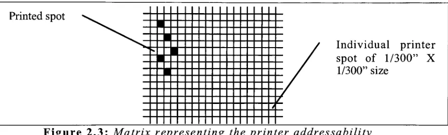
Whether AM

or

FM,

a

digital

halftone

is

designed

based

on a

matrix

representing

the

addressability

of

the printer,

as

illustrated

printer,

and

therefore

each

individual

element of

the matrix,

called

printer

spot,

is

of

the

size 1/300" x

1/300".

Each

element

in

this

matrix represents a

location

where a

dot

of

ink

could

be

placed or

not placed.

Different

types

of

digital halftone

algorithms

have been

developed

to

control

the

placement of

ink (or colorant) dots.

Printed

spot

T

H

TTItmITm

|Trr /

Individual

printer ^

>.

~P

11

/

spot of

1/300"

X

J-111

/

1/300"

size

Figure

2.3: Matrix representing

the

printer

addressability

According

to

the

screening

technique

used

the

digital halftone

can

be divided into

two

classes:

(a)

clustered and

(b)

dispersed.

2.2.3 Clustered Dot

This

is

the

most

frequently

used

technique

in

the

publishing

and

graphic arts

industries. Digital halftones

are produced

by

breaking

the

output

image down into halftone

cells,

where each cell can [image:26.531.52.511.243.382.2]

several printer pixels

(individual

addressable

cells shown

in

the

Figure 2.3).

These

pixels are either

turned

on

(making

them

black)

or

turned

off

(leaving

them

white)

by

the

printer

(laser beam

or

ink-jet

printhead).

In

a

binary

printer, the

number of

tones

that

can

be

reproduced

is limited

by

the

size of

the

cell.

A

cell

containing

n x n printer

elements will produce n2

+

1

gray levels.

For

example,

a

2x2

cell

can reproduce

5 gray

tones.

SB1

For

a given

tone to

be

reproduced,

it

must

be decided

whether each

pixel

in

the

cell should

be black

or white.

For

that purpose,

a

threshold

matrix

is

used whose elements correspond

to

each pixel of

the

cell.

These

thresholds

determine

the

gray

tone

at which

the

printer pixel

is

turned

on.

For

example,

for

a reflectance

gray

value

of

10

percent

(0

<

I

<

100),

all elements with a

threshold

value,

T,

less

than

or equal

to

10

will

be

turned

on.

Thus,

the

entire output

plane

is

covered with regular patterns of

threshold

values.

That is

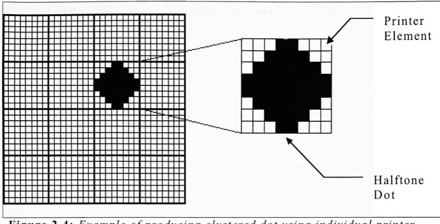
Printer

Element

Halftone

Dot

Figure

2.4: Example of producing

clustered

dot

using individual

printer

spots

The

reproduction process

is

to

assess each pixel of

the

output

plane,

and compare

the threshold

value

to the

gray

value of

the

input image

to

determine

which pixels are

turned

on.

The

condition used

is

given

by:

{0,

if

I(i,j

l,ifl(ij

0,ifI(ij)sT(ij)

B(ij)=

1

[image:28.531.40.494.79.310.2]

B(i,j)

is

the

output

value,

I(i,j)

the

input

gray

level

and

T(i,j)

the

threshold

value

The

reason

that this

method

is

called clustered

dot is

due

to

the

structure of

the threshold

matrix.

Thresholds

are ordered such

that

each subsequent

tone

would result

in

adjacent pixels

being

turned

"on" at

discrete locations in

printable area.

This

results

in

a

pattern of

dots

that

change

in

size as

the

tone

level increases.

2.2.4 Dispersed Dot

The only

characteristic of

dispersed dot

that

is different from

the

clustered

dot is

the

threshold

matrix.

In

the

previous

method,

the

matrix elements with close values were grouped

in

the

matrix.

In

the

dispersed

method,

the threshold

values are

uniformly distributed

in

the

matrix.

The

generation of

the

output

image is

the

same as

in

the

clustered

dot

method.

Tone

values are compared with

threshold

values and pixels are

turned

on or

left

off accordingly.

The

commonly

used

threshold

matrix

for dispersed dot

is

defined

by

Bayer

(Bayer,

1973).

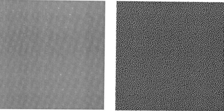
Figure

2.5

shows a

gray ramp

created with

^'SS&S.:':-::-::::

riitl.titi't'iTiTiT TiiTi-T ill- - -! **

(a)

Figure

2.5:

Gray

wedge printed with

(a)

Clustered dot

(b)

Dispersed

dot

2.2.5

Noise

Power

in Halftone Images:

The

halftoning

process creates an

illusion

of

continuity

of

tone

only if

the

halftone dots

are smaller

than the

eye can see.

A

5x5

clustered

halftone dot

printed with either a

300

or

600 dpi

printer will result

in

visually

detectable

dots.

The

magnitude of

spatial variations

in halftone

systems

is

often represented as

the

Root Mean

Squared

(RMS)

deviation

in

the

reflectance of

the

image.

This is

called

the

noise of

the

image,

o,

and

a2

is

called

the

power

of

that

image.

The

magnitude of

the

noise power varies with spatial

frequency.

The

frequency

spectrum of noise power

is

called

the

noise power

spectrum,

or sometimes

the

Wiener

spectrum

The human

visual system attenuates

the

noise power of a

halftone

at

higher frequencies.

This is

another

way

of

saying

that

if

the

halftone dots

are small

enough,

they

will

be

too

small

to

be

seen

by

the

human

eye.

If

significant

low

frequency

power

is

present

in

the

halftone

image,

it

will

generally be visually detectable

and

potentially

disturbing.

The

halftoning

algorithms

that

create

patterns with

less

power at

lower frequencies

and move

the

power

to

higher frequencies generally

produce

better

looking

images.

The

process of

moving

power

to

higher frequencies is

called

blue

noise

shifting.

More

information

on

this

can

be found in

reference:

Ulichney,

1987.

Well

defined

masks

for dispersed dot

halftoning

can shift

halftone

noise

to

higher frequencies.

Another

algorithm

for digital

halftoning

called error

diffusion

also can shift noise

to

higher frequency.

2.2.6

Floyd

Steinberg

halftone:

The

main

idea behind

the

error

diffusion

technique

is

to

compute

the

best

approximation

for

each output pixel

(whether

to

print

it

or not

to

print

it),

to

determine

the

error

between

the

actual

value and

the

output value and spread

it

to the

neighboring

pixels.

Steinberg

in 1975

(Floyd-Steinberg,

1975, Floyd-Steinberg,

1976)

and

is

often referred

to

as

the

Floyd-Steinberg

algorithm.

This

algorithm

transforms

a

gray

scale

image, I,

with reflection

gray

values

in

the

interval [0

<

I

<1],

to

a

black-and-white

image,

B,

with values of either

0

or

1.

The

psuedocode

describing

the

error

diffusion

algorithm

is

shown

below:

for every

pixel position

i,j

in I

if

I[i][j]

<

0.5

then

B[i][j]

=

0 (print

a

dot

of

ink)

else

B[i][j]

=

1

(do

not print a

dot

of

ink)

error =

I[i][j]

B[i][j]

distribute

the

error

among

unprocessed neighbors of

i,j

The

order of pixel visitation

generally

takes

the

form

of raster

processing:

for

(

i

=

0;

i

<

i_max;

i

+ +

)

{

for

( j

=

0;

j

<

j_max;

j++

) {

process pixel

i,j

}

}

The

input

and output

image dimensions

are

i_max

by

jmax.

ordering

and

distributes

the

error

to

four

unprocessed neighbors of

I[i][j]

according

to the

following

kernel:

1_

16

P

7

3

5

1

where

P

denotes

the

pixel

currently

being

processed.

The

neighbors can

be

written as:

I[i][j

+

lj

=

I[i][j

+

1]

+ error *

7/16

I[i+l][j-l]

=

I[i+l][j-l]

+

error *

3/16

I[i+l][j]

=

I[i+l][j]

+ error *

5/16

I[i+l][j

+

l]

=

I[i+l][j

+

lJ

+ error *

1/16

Although

an

image

produced

through this

algorithm

has only

two

levels,

the

visual appearance captures

the

full

grayscale range

and

detail

of

the

original

image.

However,

the

image

processed

using

the

Floyd-Steinberg

algorithm

is

often

found

to

contain worm

like

artifacts

in very dark

and

very light

regions.

A few

samples of

halftone images

created

through

[image:34.531.76.463.294.485.2]

2.3

Literature

review of

tone

reproduction

behavior

of

halftones

Many

researchers and authors

have

contributed

to

a more

thorough

understanding

of

the

optical properties of

halftone images.

This

section reviews

the

literature

on

halftone

models.

2.3.1

Murray-Davies

equation

An

ideal halftone image

contains

dots

of reflectance

R;

on

paper of reflectance

Rp.

Based

on

the

law

of conservation of

energy,

one would expect

the

total

reflectance of

the

image, R,

to

be

the

sum of

the

photon

energy from

the

dots

and

from

the

paper

between

the

dots.

This

is

expressed

in

equation

(2.1)

where

F

and

(1-F)

are

the

area

fractions

of

the

dots

and

the paper,

respectively.

Equation

(2.1),

is

often called

the

Murray-Davies

equation

(Murray,

1936).

R=F-Ri+

(1-F)

Rp

(2.1)

In assuming

the

amount of reflection

is

linearly

dependent

on

Murray-Davies

equation

inherently

assumes

that the

halftone

dots

are

spatially

uniform,

are well

defined,

the

absorption probabilities

Ri

and

Rp

are constants

independent

of

the

value of

F,

and

only direct

reflection occurs

in

the

surface

(i.e. before reaching

the

observer

light does

not reflect more

than

once

from ink

or paper surface).

In

reality,

this

is far from

true.

If

one writes equation

(2.1)

as shown

in

2.2,

where

Rk

is

Rj

at

F

=

land

Rg

is

Rp

at

F

=

₀

then

the

equation

does

a

very

poor

job

of

modeling R

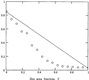
versus

F. This is illustrated in

Figure 2.7.

Reflectance,

R

0.2

0.4 0.6

Dot

area

fraction,

F

0.3

Figure

2. 7: Reflectance

vs

Dot

area

fraction,

individual

points are

the

measured

data

and continuous

line

represents

Murray

Davis Equation

2.3.2

The Yule-Nielsen

equation

It

is generally

observed

that

a printed

image

appears

darker

than

one would expect

based

on

the

nominal size of

the

dot intended

by

the

printing

process.

This

phenomenon

is

referred

to

as physical

dot

gain and

is

the

difference

of

the

measured

dot

area

fraction, F,

and

the

nominal

dot

area

fraction,

Fn

(signal

sent

to the

printer). [image:37.531.154.443.88.350.2]

printers,

physical

dot

gain

is

caused

in

part

by

local dispersion

of electric charge on

the

photo conductor

drum,

which causes unwanted

toner

particles

to transfer

onto

the

paper.

If

one uses

the

actual

dot

area,

F,

rather

than the

value sent

from

the

computer

to the

printer,

F,

equation

(2.1)

still

generally

results

in

a value of

R

that

is

lower

than the

measured value of

R.

This

effect,

which

is

different

from

physical

dot

gain,

is

called

optical

dot

gain or

the

Yule Nielsen

effect

(Yule-Nielsen,

1951).

An

empirical

function

often

found

to

be

a useful model

for

halftones is

the

Yule-Nielsen Equation (2.3).

R

= F-Rk^₊(1-F)-R/"

(2.3)

Equation

(2.3)

is

an empirical equation and

has been

found

quite successful

to

describe

the

nonlinear

relationship between R

and

F.

Moreover,

it is

common practice

to

use

the

nominal

dot

fraction, Fn,

from

the

printer

instead

of

F

in

equation

(2.2)

and

empirically

correct

for both

physical and optical

dot

gain.

The

value of n can

be determined experimentally

to

achieve

the

best

fit

between

equation

(2.2)

and measured values of

R

and

F

or

Fn.

The

study

performed

by

Ruchdeschel

and

Hauser

showed

that

1<

n <

2

(Rockdeschel-hauser,

1978).

[image:39.531.74.440.87.224.2]

Figure 2.8: R

vs.

F

modeled

by

Yule-Nielsen

equation

for

n=

1

and n=

l

.7.

Each different printing

process

has

its

own mechanistic causes

for

physical

dot

gain.

However,

optical

dot

gain

has

a single cause

that

is

common

to

all methods of

printing

on paper.

Optical dot

gain

is

caused

by

the

lateral scattering

of

light

within

the

paper

substrate.

(Yule-Nielsen,

1 95 1

_,

Arney-Engeldrum-Zeng,

1995).

Mechanistic

studies

have

shown

that

if

the

scattering distance

of

the

light in

the

paper

is

long

relative

to the

size of

the

halftone

dots,

then the

Yule-Nielsen

equation

is mechanistically

correct with n =

2

(Engeldrum,

1994). For

shorter

scattering

distances,

the

Yule-Nielsen

equation

is only

an empirical approximation of optical

dot

gain,

and numerous authors

have

published other models of

R

versus

2.3.3

Recent developments

in

mechanistic

halftone modeling

The Murray-Davies

equation

is

essentially

an expression of

the

law

of conservation of energy.

If

a

halftone image

consists of

two

reflection

populations,

R,

and

Rp,

then the

Murray-Davies

equation

(2.1)

must

be

correct,

and

the

non-linear

relationship

between

R

and

F

must

be

caused

by

a non-linear

relationship

for

R;

vs

F

and/or

Rp

vs

F.

Experimentally,

both

R;

and

Rp

are observed

to

vary

with

F

Thus,

a mechanistic model of

R

versus

F

can

be

developed

if

the

functions

for

R;

vs

F

and

Rp

vs

F

can

be

modeled.

Halftone

models of

this

kind

have

been

reported

by

Arney,

et al.

(Arney-Engledrum-Zeng,

1995,

Arney-Yamaguchi,

1999,

Arney-Tsujita,

1999).

The

Ri

vs

F

and

Rp

vs

F

models were

initially

derived

empirically based

on measured

data

on

R;

vs

F

and

Rp

vs

F

Instead

of a single empirical n

factor,

the

model contains

two

empirical

parameters w and v.

Parameter

v relates

to the

distribution

of

colorant within

the

dot

and w relates

to the

optical spread

function

of

the

paper.

Estimates

of

these

parameters are chosen

empirically

to

fit image

microstructure

data

on

R;

vs

F

and

Rp

vs

F

(Arney-Eengledrum-Zeng,

1995,

Arney-Yamaguchi,

1999,

Arney-Tsujita,

reflectance, R

versus

F

data

as well as with

R;

vs

F

and

Rp

vs

F.

This

model was also applied

in

the

analysis of

the

halftone data

generated

in

the

current

thesis

project.

Results

will

be

presented

in

subsequent sections.

Further

work reported

in

the

literature

has

explored

the

mechanistic

relationship between

the

area

fraction, F,

and

the

reflectance values of

R;

and

Rp.

This

work

involves

mean

level

probability

functions,

P,7.

The

values of

P;j

represent

the

probability for

the

scattering

of

light from

region

i

of area

fraction

/,

to

_region

j

of area

fraction,

/}

(Rogers, 1998, Arney-Wu-Blehm,

1998).

For

an

ordinary black &

white

halftone for

example,

F

-fi

and

(1-F)

=

f0.

Previously,

the

P,7

functions

were written

empirically

to

fit

observed

data

or

determined

by

convolution calculations

involving

the

paper point spread

function, PSF,

and

the

transmittance

geometry

of

the

halftone

pattern,

T(x,y).

Recent

work shows

that

Ptj

can

be deduced from symmetry

properties of

light scattering in

paper and

symmetry

properties of

the

halftone

pattern

(Arney-Yamaguchi,

1999).

A

subsequent publication also shows

how

to

account

for

higher ink

opacity

and softer

dot

edges

(Arney-Tsujita,

2.3.4

The

probability

model used

in

this

project

Tone

reproduction characteristics of

halftone

images

can

be

modeled with

knowledge

of

the

probability

function,

P0o,

for light

to

reflect

from

the

paper

back

out

between

the

halftone

dots

after

having

entered

the

paper

between

the

halftone dots

(Arney-Yamaguchi,

1999).

The

other

probability

functions

are related

to

Poo

through

equations

(2.4)

and

(2.5).

Note

that

fi

=

F

and

f0

=

(1-F),

so

the

probability

values,

P;j,

are

functions

of

F.

Arney

and

Yamaguchi

also

demonstrated

that

the

reflectance

functions,

R;

and

Rp

vs

F

can

be

calculated

from

the

probability

functions

as shown

in

equations

(2.6)

and

(2.7),

where

To

and

Ti

are

the

transmittance

values of material above regions

0

and

1

respectively.

In

general,

one assumes

Beer-Lambert

colorant

layer

of

transmittance

Ti.

For

a single

ink

system,

To=l

is

the

transmittance

of air.

Pio

=

1

-Poo

Pn

=

l-(l-Poo)-(fo/fi)

Rp=Rg-T0-(Poo-(T0-T1)

+

T,)

Ri=RB-Tr(Pir(Ti-To)

+

T0)

(2.4)

(2.5)

(2.6)

Thus,

with

knowledge

of

Poo

versus

F

one can model

R;

and

Rp

versus

F

and

then

R

versus

F.

2.3.5

Modelling

P00

for Different Halftone

Systems

Based

on experimental and

theoretical

studies reported

for

a

variety

of

different

types

of

halftone

systems,

P0o

versus

F

functions

can

be

modeled as shown

in

equations

(2.10)

and

(2.11)

(Arney-Wu-Blehm,

1998).

Poo=

1

_w(l

(1-F)B)

(2.10)

Poo=l

F-(2

Fw

(1

F)w)

(2.11)

Equation

(2.10)

describes

FM

halftones

such as

those

produced

by

the

Floyd-Steinberg

algorithm.

Equation

(2.11)

describes

clustered

dot halftones.

In

both

cases w

is

a parameter

Oswsl

related

to

the

degree

of

light scattering in

the

paper.

(Arney-Arney-Katsube-Engledrum,

1996).

The

case w=\, corresponds

to

infinite light

scattering distances in

paper,

and w=0 represents zero scattering.

The

term

B

is

an empirical

term

adjusted

to

fit

the

data.

Modeling

is done

by

first selecting

the

appropriate expression

for

Poo

and

using it

to

calculate equations

(2.4), (2.5), (2.6),

and

(2.7).

The

results are

then

used with equation

(2.1).

The

result

is

a

uniform

ink distribution in

the

printed

dots.

If

the

ink

has

a

significant

scattering

coefficient or

if

the

ink

is

not

uniformly

distributed

across

the

halftone

dot,

then

modifications

can

be

made

as

described

in

the

following

section.

2.3.6

Ink

Scattering

and

Dot Sharpness

The

following

techniques

have been

shown

to

be

useful

modifications

to the

halftone

model

(Arney-Tsujita,

1999).

First,

the transmittance

of

the

air

is

To

=

1 in

equations

(2.5)

and

(2.7).

If

the

ink has

a significant

scattering

coefficient, then

the

Beer-Lambert

assumption

does

not apply.

In

such cases one can

define

the

ink

transmittance

as

Ti=Tkm

where

Tkm

is

the

transmittance

of an

absorbing

and

scattering ink

given

by

Kubelka-Munk

theory,

equation

(2.8).

Tkm

= "

(2-8)

a

sinh(bSx)

+

b

cosh(bSx)

In

this equation, x=

ink layer

_{thickness at}

F=l

K

=

Kubelka-Munk

_{absorption coefficient}

in

mm"1

S

=

Kubelka-Munk scattering

coefficient

in

mm"'

a=

(K/S+l)

and

b

=

(a2-l) 5

In

addition

to

scattering

of

light in

the

ink,

the

sharpness of

is

often observed

experimentally that

dot

edges are not

sharp but

show a progressive

decline

in ink amount,

feathering

into

white

between

the

dots.

Such

systems

do

not show

clearly defined

edges,

and

the

concept of a

distinct

dot

edge

is

more

difficult

to

apply

with

confidence.

In

the

current work

the

dot

edge was

defined

as

the

region of most rapid spatial change

in reflectance,

dR/dx

=

maximum.

This may

not

be

the

region where

ink quantity

reaches

zero,

but it is

a region

that

can

be identified

and measured

repeatably.

Experimentally

the

dot

edge

is determined in image

micrographs

by

a

histogram

analysis.

The

edge

is identified

as

the

value of

R

at

lowest

occurrence where

dH/dR

=

minimum

for

histogram H(R).

Segmentation

at

this

value of

R

provides a

repeatable measure of

dot

area

fraction,

F.

A

consequence of

defining

the

dot

edge

in

this

way is

the

need

to

modify

the

definitions

of

To

and

Tt

in

equations

(2.6)

and

(2.7).

We define

T0

and

Ti

as shown

in

equations

(2.9

and

2.10),

T0=

1-(1-TKM)-(1-(1-F)V)

(2.9)

Ti

=

1-(1

Tkm)-Fv

(2.10)

where

Tkm

is

defined

in

equation

(2.7).

The

value of v

is

an

model and experimental

data.

A

value of v =

0

corresponds

to

perfectly

sharp dot

edges.

The

procedure

for

fitting

the

model

to

experimental

data

was

as

follows.

Starting

values of w and v were selected.

Then

the

model

for

Poo

was chosen

(equation

(2.10)

or

(2.11)).

Scattering

and absorption coefficients

S

and

K

for

the

ink

were assumed and

applied

to

equation

(2.7).

Then

equations

(2.9)

and

(2.10)

provided

values of

TO

and

TI

which were used

instead

of

T0

and

Ti

in

equations

(2.4), (2.5), (2.6),

and

(2.7).

Finally,

the

values of

R;

and

Rp

from

(2.6)

and

(2.7)

were used

in

equation

(2.1)

to

calculate

R.

This

was repeated

for different

values of

F from 0

to

1

.

The

values

of

w,

v,

K

and

S

were selected

to

minimize

the

RMS deviation

between

the

model and

the

data

simultaneously

for

R;

vs

F,

Rp

vs

F,

Chapter

3:

Behavior

of

halftones

printed

on

EP

printers

This

section

discusses

the

observed

behavior

of

the

printed

halftones

on

both 600 dpi

and

300 dpi EP

printers.

In

the

first

subsection

the

histogram

characteristics

of

these

samples are

discussed.

When

histograms

of

Floyd-Steinberg

halftone

patterns

are

observed,

they

differ

significantly from

the

ideal

halftone

system

behavior

given

by

the

Murray-Davies

equation

(2.1).

The

causes

for

this

phenomenon are

discussed

in

the

following

subsection.

The

last

subsection contains results of

applying

the

halftone

model

described in

section

2.3.4

to

characterize

the

behavior

of

the two

printing

systems chosen

for

this

study

3.1 Tone behavior

of

halftones in histograms

The quality

of printed

halftone images is

largely

controlled

by

the

spatial

distribution

of

gray

levels

within

the

halftone

structure.

The

distribution

of

the

gray

levels

in

printed

halftones

can

be

observed

in

the

histogram

of

images

captured

using

a

CCD

camera

with reflectance values

from

0

to

1.

The

histogram

gives

information

on

the

fraction

of

total

pixels

in

the

captured

image

of

that

particular reflectance value

(note:

pixels referred

in

this

statement are

the

pixels of

the

image

through

a

digital

camara and

not of

the

original

image

that

was printed).

The histogram is

useful

for measuring

specific attributes

for

microdensitometric analysis.

Commonly

applied metrics

include

the

halftone

dot

area

fraction, F,

the

mean reflectance of

the

paper

between

the

halftone

dots, Rp,

and

the

mean reflectance of

the

dots,

R;.

The

procedure

for measuring

these

metrics are

described in detail in Appendix

A,

section

A.l.

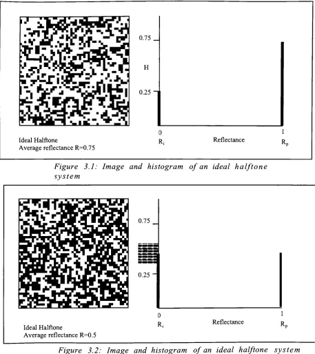
If

we consider

the

histogram

of

the

ideal halftone

system

(a

system

that

obeys

Murray-Davies

Model,

equation

2.1),

its

total

pixel population should

be localized

at

two

specific points

in

the

histogram:

colorant reflectance

R;

and paper reflectance

Rp. Two

examples of such a system are shown

in Figure 3.1

and

3.2.

These

are

halftone images

of

nominally

uniform

tone

patches of constant

reflectance.

The first image has

an average reflection of

0.75

and

the

second

has

average reflection of

0.5.

By increasing

the

number

of

black

dots,

the

fraction

of

the total

area covered

by

colorant

is

increased,

which results

in

a

lower

reflectance of

that

area of

the

pixel

population at

Ri

and a

corresponding

decrease

in

population at

0.75

_

H

0.25

~

Ideal Halftone

Average

reflectance

R=0.75

0

Reflectance

1

R

Figure

3.1: Image

and

histogram

of

an

ideal

halftone

system

0.75

0.25

-Ideal

Halftone

Averagereflectance

R=0.5

0

R,

Reflectance

1

Rn

Figure

3.2:

Image

and

histogram

of

an

ideal

halftone

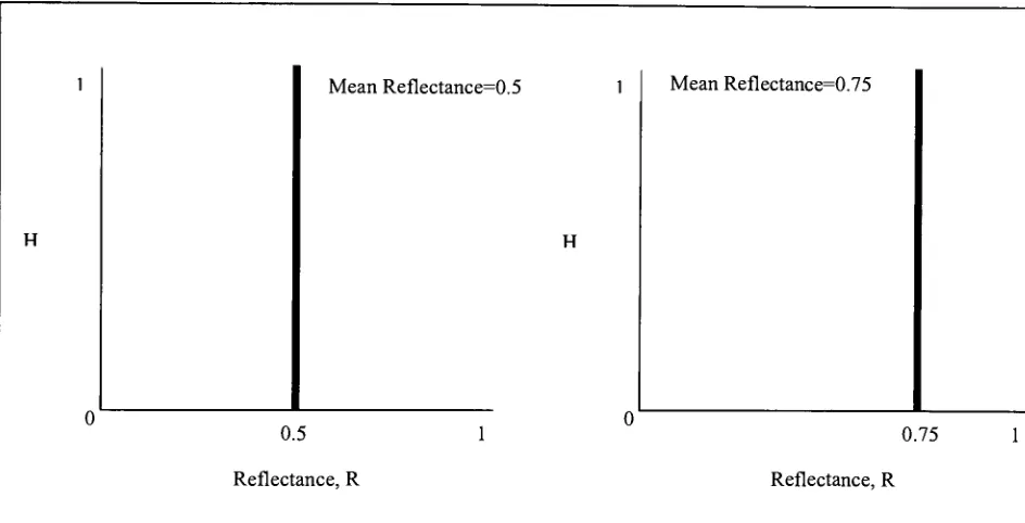
system [image:50.531.38.495.76.589.2] [image:50.531.43.492.83.311.2]

Consider

the

histogram

of an

ideal

continuous

tone

image

of a

single

tone.

The

total

pixel population

in

a

histogram

would

be

situated

at a single reflectance

value,

at

the

reflectance

of

the

image,

R. As

the

reflectance of

the

image

changes,

the

population

would move

to

the

new reflectance value.

1

H

Mean Reflectance=0.5

1

H

Mean Reflectance=0.75

0

0

0.5

1

0.75

1

Reflectance,

R

Reflectance,

R

Figure

3.3: Histograms of

ideal

continuous

tone system,

at

R

=

0.5

and

R

=

0.75

To

summarize

the

differences in

the

histogram behavior

of

both

ideal

halftone

and continuous

tone

systems:

in

an

ideal

[image:51.531.39.511.220.461.2]

populations

at

R;

and

Rp,

whereas

in

an

ideal

continuous

tone

system

the

pixel population moves

along

the

R

axis.

The histograms

of real systems

do

not

have

tightly

populated,

bimodal

distributions.

Due

to

local image

variations

(noise),

the

physical spread of

the

edges of

halftone

dots,

and

the

optical

scattering

of

light

in

the paper, the

printed

halftones

have

rather

broad

population

distributions.

Two

examples of such

histograms

are shown

in Figures 3.4

and

3.6

for

samples printed on a

300-dpi

EP

printer

using

a

Floyd-Steinberg

halftoning

algorithm.

An

increase

in

Fn

(nominal dot

fraction

sent

to

the

printer)

results

in

an

increase in

the

pixel population of

the

lower R distribution

and a

decrease in

the

higher R distribution.

This

is

a characteristic of an

ideal

halftone

system.

However,

the

reflectance values at which

the

two

local

maxima occur change with

the

change

in Fn.

Thus

the

real

system shown

in figures 3.4

and

3.6,

demonstrates

characteristics of

both

an

ideal halftone

and a continuous

tone

system.

Histograms

of samples printed

using

Floyd-Steinberg

with a

600-dpi

printer are shown

in figures 3.5

and

3.7.

The dots

are

visible and

easily distinguishable from

surrounding

paper

in

these

images.

Unlike

the

histograms

of

the

300-dpi system,

these

one

histogram

maximum and a

broad,

asymmetrical

distribution.

As

Fn

is

changed,

the

value of

R

at

the

peak changes.

This

behavior

is

W~"F

*

'**

flf*#l

H

1 mm

Reflectance,

R

Captured

image

of printed_sample,

F=0.1

Figure

3.4:

Histogram

of

Floyd-Steinberg

halftone

(Fn

=

0.1)

printed on

300 dpi EP

printer

*

%

r^--'.'-"'*'".# "*'

iff

^

.#-.

,

-*W

i

;*

a

*

H

* ? *>

3

* -,,, *

* . --.

^

0.5mm

Captured

image

of printedsample,

Fn=0.0625

Reflectance

R

Figure

3.5:

Histogram

of

a

Floyd-Steinberg

halftone

printed on a

600

[image:54.531.51.469.76.333.2]

H

1 mm

Reflectance,

R

Captured image

of printedsample,

Fn=0.3

Figure

3.6: Histogram

of

Floyd-Steinberg

halftone

(F

=0.3)

printed on

300 dpi EP

printer

H

0.5mm

Reflectance R

Captured image

of printedsample, Fn=0.44

3.2

Observation

of

printed

images

at

microscopic

level

and

point

spread

function

of non-coated paper

A

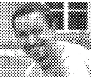
comparison of microscopic views of samples printed with

600 dpi

and

300 dpi EP

printers

is

shown

in

figure

3.8.

The

samples

printed on

the

300 dpi

printer

have

well

formed

dots. Toner

particles are

scattered,

but

the

amount of

scattering is

not as

significant as

it is for

the

600dpi

printer s