The Least Square free Primitive Root Modulo a Prime

The Least Square-free Primitive

Root Modulo a Prime

Morgan Hunter

October 2016

A thesis submitted in partial fulfilment of the requirements for the degree of

Bachelor of Science (Honours)

Declaration

The work in this thesis is my own except where otherwise stated.

Acknowledgements

I would really like to thank my supervisor Tim Trudgian. He suggested a great topic for my thesis that I have found very interesting and rewarding to study. I would also like to thank him for funding my MSI Honours Scholarship, without which I would not have been able to complete honours this year.

I would also like to thank Mark Lawrenson who assisted with the implementation of the algorithm.

Abstract

The aim of this thesis is to lower the bound on square-free primitive roots modulo primes. Letg2(p) be the least square-free primitive root modulop. We have proven the following two theorems.

Theorem 0.1.

g2(p)< p0.88 for all primes p.

Theorem 0.2.

g2(p)< p0.63093 for all primes p <2.5×1015 and p >9.63×1065.

Theorem 0.1 shows an improvement in the best known bound while Theorem 0.2 shows for which primes we can prove the theoretical lower bound.

After some introductory information in Chapter 1, we will start to prove the above theorems in Chapter 2. We will introduce an indicator function for primitive roots of primes in §2.1 and together with results from §1.2.1, §1.2.3 and §1.2.4 we will outline the first step in proving a general theorem of the above form. The next two stages in the proof will be outlined in Chapter 3. These two stages require the introduction of the prime sieve. Before defining the sieve in §3.2 we will introduce thee−free integers which will play an important role in defining the sieve.

In §3.2 we will obtain results that do not require computation, including Theo-rem 0.2. An algorithm is then introduced in§3.3 which is the last stage of the proof. There we will complete the proof of Theorem 0.1.

Contents

Acknowledgements v

Abstract vii

1 Introduction 1

1.1 Notation . . . 2

1.2 Primitive roots . . . 2

1.2.1 The M¨obius and Euler totient functions . . . 4

1.2.2 Square-free integers . . . 5

1.2.3 Dirichlet characters . . . 7

1.2.4 P´olya–Vinogradov inequality . . . 11

2 Least square-free primitive root 17 2.1 Results without sieving . . . 19

3 Sieving 29 3.1 e-free integers . . . 30

3.2 Results with sieving . . . 35

3.3 Results using the prime divisor tree . . . 40

3.3.2 Results . . . 50

4 Conclusion and future work 51

4.1 Conclusion . . . 51

4.2 Future work . . . 52

1

Introduction

There are many interesting questions concerning the distribution of primitive roots modulo primes. In particular we are interested in the least prime primitive root of a prime. The asymptotic bound on the least prime primitive root is quite weak, and very difficult to improve, so in this thesis we will instead concentrate on a more general type of primitive root. We will be studying the least square-free primitive root modulo a prime.

Before we are able to bound the least square-free primitive root, we need to understand what a primitive root is and what basic properties it has. After outlining this in§1.2 we will introduce some arithmetic functions that are important in later chapters. In §1.2.4 we introduce the famous P´olya–Vinogradov inequality. This inequality is crucial in lowering the bound on the least square-free primitive root of a prime.

1.1

Notation

Throughout this thesis standard analytic number theory symbols are used. We will use the following shorthand: [x] denotes the integer part ofxand (a, b) denotes the greatest common divisor ofaandb. We will use ‘O’-notation andandsymbols as follows: for functionsf(x) andg(x) the notationf(x) =O(g(x)) andf(x)g(x) mean that there exists a positive constantM such that|f(x)/g(x)|< M whenx is sufficiently large. The relationf(x)g(x) is interpreted as g(x)f(x).

1.2

Primitive roots

In order to define what a primitive root is we need to define the order of an integer.

Definition 1.1. Let (a, m) = 1, then theorderofa(modm) is the smallest integer

ksuch that ak ≡1 (mod m) and is denoted ordm(a) =k.

Proposition 1.1 (Theorem 8.4 from [30]). Let k be a positive integer. If ordma=d

then

ordm

ak= d (d, k).

In particular, there are φ(d) distinct powers ofa with orderd.

Definition 1.2. We sayris a primitive rootmodulom (alternatively,r is a prim-itive root of m) if ordm(r) = φ(m). Equivalently, r is a primitive root modulo m

if it generates the set of integers coprime to m. In particular, for all a such that (a, m) = 1 there exists k such thatrk≡a(mod m).

Remark 1.1. Proposition 1.1 implies that if r is a primitive root modulo m then

rk is a primitive root modulo m if and only if (k, φ(m)) = 1. Therefore if we have found one primitive root modulo m, we can generate all other primitive roots ofm.

Example 1.1. Let us find the primitive roots of 7. Since 7 is prime, order is defined for all positive integers less than 7. We have

21≡2,22 ≡4,23 ≡1

so 2 is not a primitive root of 7. Next we try 3,

so 3 is a primitive root of 7. Now that we have a primitive root we can generate all other primitive roots, φ(7) = 6 so k = {1,5}. Therefore the only other primitive root modulo 7 is 35_≡5.

The fact that a primitive root modulomgenerates the set of all coprime integers tom leads to the following definition.

Definition 1.3. Let r be a primitive root modulo m. Then for all integers a such that (a, m) = 1, we define the base r discrete logarithmof a, to be the unique integerk∈ {1, . . . , φ(m)} such that

rk≡a(modm).

We denote this indr(a) =k. The baser discrete logarithm is also known as the base r index.

Note that it follows directly from Remark 1.1 that ifgis a primitive root modulo

m, then a is a primitive root modulo m if and only if (indg(a), φ(m)) = 1. The

discrete logarithm not only provides some useful notation, but also the discrete logarithm moduloφ(m) shares the basic properties of logarithms.

It may be tempting to assume that all integers have primitive roots, however this is not true.

Example 1.2.

Considerm= 8.

Here we haveφ(8) = 4 and from Definition 1.1 the order is only defined for coprime integers to 8. Therefore we are left to considerr = 1,3,5,and 7 as possible primitive roots. However

12 ≡32 ≡52≡72≡1 (mod 8),

so ord8(r) = 2 6= 4 for all r = 1,3,5,7 and therefore there are no primitive roots

modulo 8.

Proposition 1.2.

1. There exist primitive roots for all primes.

2. Powers of 2, except for 1,2 and 4, do not have primitive roots.

3. There exist primitive roots for all powers pk and 2pk where p is an odd prime and k≥1.

As we can see, our example from above fits into category 2, as 8 is a power of 2 and therefore does not have any primitive roots. From this point onwards we will be focusing on primitive roots modulo primes.

By Definition 1.2 we know that r is a primitive root modulo a prime p if

{rk (modp)|k= 1, . . . , p−1}={1,2, . . . , p−1}.

and we also have that every prime has exactly φ(p−1) primitive roots (Chapter 8.2 of [30]). As we mentioned at the start of this chapter, we are interested in the distribution of primitive roots modulo primes. However to study the primitive roots of an unknown prime p we first need some background on arithmetic functions. These play an important part in later chapters of this thesis

1.2.1

The M¨

obius and Euler totient functions

As mentioned above, to study primitive roots we require some background informa-tion on particular arithmetic funcinforma-tions. Arithmetic funcinforma-tions are real or complex functions that are defined on the set of natural numbers. In this section we will look at the M¨obius function and the Euler totient function. In §1.2.3 we will introduce Dirichlet characters, which are also arithmetic functions. The properties of Dirichlet characters will be important in Chapter 2.

Definition 1.4.

The M¨obius function is defined by

µ(n) =     

   

0 ifp2|nfor any primep,

(−1)k ifnis the product of kdistinct primes, 1 ifn= 1.

The Euler totient functionis defined by

φ(n) = #{k∈_Z|1≤k≤n, (k, n) = 1}.

These two arithmetic functions will appear repeatedly in the following chapters and some of their important properties are stated below.

Proposition 1.3. Bothµ(n) and φ(n) are multiplicative.

That is if (n, m) = 1 thenµ(nm) =µ(n)µ(m) and φ(nm) =φ(n)φ(m). Proof. See Chapter 6 in [30].

Remark 1.2. If (a, b) >1 thenµ(ab) = 0. This follows because there exists c such thatc|aand c|band therefore c2_|ab.

Proposition 1.4 (Sums over divisors). Let n≥1. Then

1. X

d|n

µ(d) =  



1 if n= 1,

0 if n >1.

2. X

d|n

φ(d) =n.

Proof. See Theorem 264 and§16.2 in [15].

An example of M¨obius inversion shows how these two arithmetic functions are related [1]. Forn≥1 we have

φ(n) =X

d|n µ(d)n

d.

Proposition 1.5.

φ(n) =nY p|n

1−1

p

,

where the product is over the distinct prime divisors ofn.

Proof. See Theorem 62 in [15].

An important application of the M¨obius function is related to square-free integers.

1.2.2

Square-free integers

For example, 42 is a square-free integer, 42 = 2·3·7, while 56 = 23·7 is not a square-free integer as 2 is a repeated prime factor.

It is clear from the above definition that all primes are square-free hence square-free integers are a weak generalisation of the primes. Recall thatµ(n) is 0 ifnis divisible by the square of a prime and ±1 otherwise. Hence one possible indicator function of square-free integers is

|µ(n)|=  



1 ifnis square-free, 0 otherwise.

Another characteristic equation for square-free integers is given by Shapiro [31]. First note that all integers ncan be expressed as n=s2q where sis an integer and

q is square-free. Therefore from Proposition 1.4 we have

X

d2_|n

µ(d) =X

d|s

µ(d) =  



1 ifs= 1,

0 otherwise.

If s = 1 then n is square-free and so a characteristic equation for square-free integers is

X

d2_|n

µ(d) =  



1 ifnis square-free,

0 otherwise.

(1.1)

Now consider the number of square-free integers less than or equal tox. We then have to consider the sum

X

n≤x n=2−free

1 = X

n≤x |µ(n)|

Lemma 1.1 (Lemma 4.2 in [3]). If x≥1 then X

n≤x

|µ(n)|= 6

π2x+P(x), with

(a) −0.103229√x≤P(x)≤0.679091√x for x≥1,

(b) |P(x)| ≤0.1333√x for x≥1664,

(c) |P(x)| ≤0.036438√x for x≥82005,

(d) |P(x)| ≤0.02767√x for x≥438653.

These explicit bounds on the number of square-free integers less than or equal toxwill be important in Chapter 2, where we obtain results on the least square-free primitive root modulo a prime. The next section introduces the Dirichlet characters which will also be important in Chapter 2.

1.2.3

Dirichlet characters

A Dirichlet character is a certain type of arithmetic function. They are important in the study of primitive roots, in particular they appear in the indicator function for primitive roots modulo a prime (2.1).

Definition 1.6. Letq be a positive integer. Then a Dirichlet charactermoduloq

is a functionχ:N→Cwith the following properties:

1. χis periodic modulo q, i.e. χ(n+q) =χ(n) for all n∈_N.

2. χis completely multiplicative, i.e. χ(nm) =χ(n)χ(m) for alln, m∈N. 3. χ(n)6= 0 if and only if (n, q) = 1.

The character

χ0(n) =

 



1 if (n, q) = 1 0 if (n, q)>1 is called theprincipal charactermodulo q.

Proposition 1.6. Let χ be a Dirichlet character modulo q. Then the values ofχ are

either0 or φ(q)th roots of unity.

It follows from Proposition 1.6 that if χ is a Dirichlet character modulo q then so is the complex conjugate χ, whereχ(n) =χ(n).

Just as we have defined the order of an integer modulo q (Definition 1.1) we can define the order of a Dirichlet character modulo q. Let χ be a Dirichlet character modulo q then the order of χ is the smallest exponent d, with d| φ(q), such that

χd=χ0.

Proposition 1.7 (§6.5 in [31]). There are exactly φ(q) Dirichlet characters modulo

q. They are denotedχ0, χ1, . . . , χφ(q)−1.In particular, given d|φ(q) there are φ(d)

Dirichlet characters modulo q of order d.

Consider all the Dirichlet characters, χ, modulo q. The possible orders of these characters are the divisors of φ(q). Letd1, d2, . . . , ds be the divisors of φ(q). Then

from Proposition 1.4 we have

φ(d1) +φ(d2) +· · ·+φ(ds) =φ(q).

Since there are φ(q) Dirichlet character modulo q, Proposition 1.4 shows that the Dirichlet characters can be partitioned according to their order.

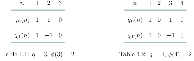
Example 1.3. When q = 1 or q = 2, φ(q) = 1 and so there is only one Dirichlet character, namely the principal character.

When q= 3 or q= 4 then there are 2 Dirichlet characters defined in Table 1.1 and Table 1.2.

n 1 2 3

χ0(n) 1 1 0

χ1(n) 1 −1 0

Table 1.1: q = 3, φ(3) = 2

n 1 2 3 4

χ0(n) 1 0 1 0

χ1(n) 1 0 −1 0

Table 1.2: q= 4, φ(4) = 2

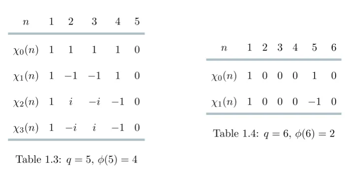
n 1 2 3 4 5

χ0(n) 1 1 1 1 0

χ1(n) 1 −1 −1 1 0

χ2(n) 1 i −i −1 0

χ3(n) 1 −i i −1 0

Table 1.3: q = 5, φ(5) = 4

n 1 2 3 4 5 6

χ0(n) 1 0 0 0 1 0

χ1(n) 1 0 0 0 −1 0

Table 1.4: q = 6, φ(6) = 2

Not only can we describe Dirichlet characters as either principal or non-principal, there are other classifications depending on the character’s specific properties. For example we can describe a Dirichlet character as either even or odd.

Definition 1.7. Let χbe a Dirichlet character modulo q. We callχ oddifχ(−1) =−1 or even ifχ(−1) = 1.

We can also define primitive Dirichlet characters, just as we defined primitive roots in§1.2. In the same way that a primitive root generates the coprime integers, all Dirichlet characters can be viewed as extensions of primitive Dirichlet characters.

Definition 1.8. Letχ be a Dirichlet character moduloq and letd|q. Then dis an

induced modulusforχif for allasuch that (a, q) = 1 anda≡1 (modd) we have

χ(a) = 1.

A Dirichlet character is called primitive if it has no induced moduli. In other words,χ is primitive if and only if for alld|q there exists anawitha≡1 (modd) and (a, q) = 1 such that χ(a)6= 1.

As we will see in later chapters, Dirichlet characters often appear to us in sums. We sometimes have to sumχ(n) overnor perhaps sum over all the Dirichlet charac-ters of the same order for a fixedn. We will see in the following part of this section some nice properties of the Dirichlet characters and their sums.

Definition 1.9. Let χbe any Dirichlet character modulo m then

G(n, χ) =

m

X

k=1

χ(k)e2πikn/m

The Gauss sum will be important in the next section as it is needed in the proof of the P´olya–Vinogradov inequality. The following proposition is important in proving the indicator function for primitive roots.

Proposition 1.8. Let Γd denote the set of all Dirichlet characters modulop of order dand define

S(d) = X

χ∈Γd

χ(n).

S(d) is multiplicative.

Proof. Let d1 andd2 be coprime integers and consider

S(d1d2) =

X

χ∈Γd₁d₂

χ(n) =χ0(n) +χ2(n) +· · ·+χφ(d1d2)−1(n).

There are φ(d1d2) = φ(d1)φ(d2) characters of order d1d2 as φ is multiplicative

(Proposition 1.3) and so there areφ(d1)φ(d2) terms in the sum.

Now let ψi, where i= 1, . . . , φ(d1), be the φ(d1) Dirichlet characters of order

d1 and letηj, wherej= 1, . . . , φ(d2), be theφ(d2) Dirichlet characters of orderd2.

Then

S(d1)S(d2) =



 X

χ∈Γd₁

χ(n) 

 

 X

χ∈Γd₂

χ(n) 

=

φ(d1) X

i=1

φ(d2) X

j=1

(ψiηj)(n).

This sum has at mostφ(d1)φ(d2) terms. Therefore if we can show that the product

of Dirichlet characters,ψη, has orderd1d2 and that the sumS(d1)S(d2) has exactly

φ(d1)φ(d2) terms, we have S(d1d2) =S(d1)S(d2).

Firstly we will show that ifψ∈Γd1 and η∈Γd2 thenψη∈Γd1d2. Let ψ ∈ Γd1 and η ∈ Γd2, then ψ

d1 _{= χ}

0 and ηd2 = χ0 where χ0 is the

princi-pal character modulo p. So (ψη)d1d2 _{= ψ}d1d2_ηd1d2 _{= χ}d2

0 χ

d1

0 = χ0 which means

ord(ψη)≤d1d2 (where ord(χ) denotes the order ofχ). Suppose ord(ψη) =K then

by the division algorithm (Theorem 1.2 in [27]) d1d2 = qK+r where q > 0 and

0≤r < K. Then

χ0 = (ψη)d1d2 = (ψη)qK+r=χ0(ψη)r= (ψη)r.

This means that if 1 ≤ r < K then ord(ψη) ≤ r < K. This is a contradiction as ord(ψη) = K. So r = 0, in particular K | d1d2. So there exists A such that

K = d1d2

A . Since the order is the least exponent, K, such that (ψη)

K _{= χ}

0, A

is the greatest common divisor of d1 and d2. So K =

d1d2

(d1, d2)

least common multiple of d1 and d2. Since (d1, d2) = 1, K = d1d2 and therefore

ψη∈Γd1d2.

Now we will prove that the sum S(d1)S(d2) has exactlyφ(d1)φ(d2) terms.

SupposeS(d1)S(d2) has less than φ(d1)φ(d2) terms, in particular there is a double

up of characters. Thenψaηb =ψcηddefines a double up in the following three cases:

(a = c and b 6= d), (a 6= c and b = d) and (a 6= c and b 6= d). Without loss of generality we assume, a 6= c. Since ψaηb = ψcηd, ψa = ψcηdη−b1 and we have two

cases, where eitherηdη−_b1 =χ0 orηdη_b−16=χ0.

Suppose ηdη−b1 =χ0 then ψa = ψc however this implies that a = c which is a

contradiction. Now supposeηdη_b−1 6=χ0 then sinceηb ∈Γd2, η −1

b ∈Γd2. So we have ηdηb−1 ∈ Γd2, that is ord(ηdη

−1

b ) = d2. If d2 = 1 then ηdηb−1 −χ0 and so d2 > 1.

Therefore by the first part of this proof ord(ψcηdη_b−1) = ord(ψc)ord(ηdη−_b1) =d1d2>

d1. However ψa =ψcηdη_b−1 and ord(ψa) = d1 which is a contradiction and so each

ψiηjdefines a unique character of orderd1d2 for all 1≤i≤φ(d1) and 1≤j≤φ(d2).

Therefore the sumS(d1)S(d2) hasφ(d1)φ(d2) unique terms.

HenceS(d) is multiplicative.

The following section will introduce a famous inequality on the sum of Dirichlet characters. This bound will play an important part in Chapter 2.

1.2.4

P´

olya–Vinogradov inequality

The P´olya–Vinogradov inequality provides a bound on the sum of Dirichlet char-acters that is independent of the interval of summation. Because of this we can use this inequality when we need to bound the sum of Dirichlet characters in§2.1. There has been extensive research done on the inequality and therefore quite strong bounds are known. We will go through some of these in this section.

Letχbe a non-principal Dirichlet character moduloqthen the P´olya–Vinogradov inequality (Theorem 9.18 in [24]) states that

M+N

X

n=M+1

χ(n) =O(√qlogq) (1.2)

for any integersM and N withN >0. Equivalently,

M+N

X

n=M+1

χ(n)

≤c√qlogq (1.3)

This inequality was independently discovered by P´olya [28] and Vinogradov [32] in 1918. Consider the trivial bound on the same sum. Since |χ(n)| ≤ 1 for all n

(Proposition 1.6) we have N X n=1

χ(n)

=|χ(1) +χ(2) +· · ·+χ(N)| ≤N. (1.4)

We can expect the bound to be much smaller for non-principal characters. There is a lot of cancellation as the sum cycles through roots of unity. For example, recall the Dirichlet characters modulo 5 from Table 1.3. Let N = 7, then we have

7

X

n=1

χ0(n) =χ0(1) +χ0(2) +· · ·+χ0(5) +χ0(1) +χ0(2)

= 1 + 1 + 1 + 1 + 0 + 1 + 1 = 6,

7

X

n=1

χ1(n) = 1−1−1 + 1 + 0 + 1−1 = 0, 7

X

n=1

χ2(n) = 1 +i−i−1 + 0 + 1 +i= 1 +i, 7

X

n=1

χ3(n) = 1−i+i−1 + 0 + 1−i= 1−i.

Note that if N = 5 then the sum equals 0 for all non-principal characters and

φ(5) = 4 for the principal character. Consider summing up to a multiple of the modulus. Letχbe a Dirichlet character moduloq, then for anyk≥1, by periodicity we have

kq

X

n=1

χ(n) =  



0 ifχ is non-principal,

kφ(q) ifχ is principal.

We can see from the above example that when χ is non-principal there is a lot cancellation however when χ is a principal character we are summing a string of ones, with zeros appearing only when (n, q)>1. Therefore we only need to bound the sum whenχ is non-principal as it is known whenχ is principal.

As a result of Montgomery and Vaughan’s work in [23] we have the following lower bound on the character sum

M+N

X

n=M+1

χ(n) √q

Hypothesis1, Montgomery and Vaughan [22] have also shown that

M+N

X

n=M+1

χ(n)

√qlog logq

for any Dirichlet character moduloq. The implicit constant for the P´olya–Vinogradov inequality can be shown to be 1 for all non-principal characters. One proof of this can be found in Davenport’s book [7]. We will prove c = 1 for all primitive char-acters as the full proof for all non-principal charchar-acters is long and can be extended from the following proof.

Theorem 1.1(Theorem 8.12 in [1]). Let χbe any primitive Dirichlet character

mod-ulo q then for all x≥1 we have X

n≤x χ(n)

<√qlogq.

Proof. Letχbe a primitive character moduloq then the finite Fourier expansion of

χ(n) (Theorem 8.20 in [1]) is

χ(n) = G(1, χ)

q q

X

k=1

¯

χ(k)e−2πink/q

where the Gauss sum is

G(1, χ) =

q

X

n=1

χ(n)e2πin/q

and ¯χis the complex conjugate of χ. Now we sum over alln≤x to obtain

X

n≤x

χ(n) = G(1, χ)

q

q−1

X

k=1

¯

χ(k)X

n≤x

e−2πink/q.

Here the sum of Dirichlet characterχ(k) is now between 1≤k≤q−1 sinceχ(q) = 0. Since we are looking for a bound we need to take absolute values, which results in

X

n≤x χ(n)

=

G(1, χ)

q

q−1

X

k=1

¯

χ(k)X

n≤x

e−2πink/q

≤ |G(1, χ)| q

q−1

X k=1 ¯

χ(k)X

n≤x

e−2πink/q

. 1

From Proposition 1.6 we have|χ(n)| ≤1 and so it follows that|χ¯(n)| ≤1 and so X

n≤x χ(n)

≤ |G(1, χ)| q

q−1

X k=1 X

n≤x

e−2πink/q

= |G(1, χ)|

q

q−1

X

k=1

|f(k)| (1.5)

where

f(k) =X

n≤x

e−2πink/q.

Now consider the functionf(k).

f(q−k) =X

n≤x

e−2πin(q−k)/q =X

n≤x

e2πink/qe−2πin=X

n≤x

e2πink/q =f(n)

which means |f(q−k)|=|f(k)|=|f(k)|. Hence

q−1

X

k=1

|f(k)| ≤ q/2

X

k=1

|f(k)|+

q−1

X

k=q/2

|f(q−k)|

= 2

q/2

X

k=1

|f(k)|. (1.6)

Now let r=e−2πik/q and a= [x] thenf(k) is a geometric series,

f(k) =

a

X

n=1

rn

with r 6= 1 since 1≤k ≤q−1 and writing t=e−πik/q _{we have r =t}2 _{and t}2 _{6= 1}

since 1≤k≤q/2. Hence

f(k) = r(1−r

a₎

1−r =

t2(1−t2a) 1−t2 =

t2+a(t−a−ta)

t(t−1_−t) =t

1+at−a−ta t−1_−t

and so using Euler’s formula,eix = cosx+isinx, we have

|f(k)|=

t−a−ta t−1_−t

=

eπika/q−e−πika/q eπik/q_−e−πik/q

= sin πka q sin πk q ≤ 1

sinπk_q

. (1.7)

Now we relax the bound on |f(k)| by using the inequality sin(u) ≥ 2u/π which is valid for 0≤u≤π/2. Since k≤q/2 then πk/q ≤π/2 and so (1.7) becomes

|f(k)| ≤ ₂1 π

πk q

= q

Substituting (1.6) and (1.8) into (1.5) we have X

n≤x χ(n)

≤ |G(1, χ)|

q 2 q/2 X k=1 q 2k

=|G(1, χ)| q/2

X

k=1

1

k

<|G(1, χ)|logq. (1.9) Sinceχis a primitive Dirichlet character moduloq, for allnsuch that (n, q) = 1 we have |G(n, χ)|=√q. A proof of this can be found in Theorem 8.11 and Theorem 8.19 from [1]. Therefore

X

n≤x χ(n)

<√qlogq.

There has been extensive work done on improving the upper bound of (1.3). These improvements are obtained from advanced methods and so they will not be proved here. In 2007 Granville and Soundararajan [11] showed that if χ has odd order then a small power of logq can be saved in (1.3). The following result was improved in 2012 by Goldmakher [10] who stated that for each fixed odd number

g >1, forχ of orderg, X

n≤x χ(n)

≤√q(logq)∆g+O(1) _{where ∆}

g = g πsin

π

g, asq → ∞.

In 2013, Frolenkov and Soundararajan [9] were able to obtain an explicit version of the P´olya–Vinogradov inequality for all non-principal Dirichlet characters. They used a result which bounds the sum (over any interval [M+ 1, M+N]) of a broader class of arithmetic functions than the Dirichlet characters to obtain the following theorem.

Theorem 1.2(Corollary 1 in [9]). Letq >100and letχbe any non-principal Dirichlet character moduloq. Then we have

X

n≤x χ(n)

< c√qlogq

where

c=

1

π√2 + 6

π√2 logq +

1 logq

The parameter, c will decrease as we takeq to be large. In particular, both the second and the third term tend to zero and c→ (π√2)−1 as q → ∞. This will be important when we use this theorem later in§2.1.

Recall the trivial bound (1.4). There are some cases where the trivial bound is lower than the bound in Theorem 1.2. Hence, we write

X

n≤x χ(n)

<min{x, c√qlogq}.

There have been many improvements to (1.3) for primitive Dirichlet characters. In particular, sharper bounds have been found when splitting the sum into the sum of either even or odd Dirichlet characters. Explicit bounds of this form have been found by Pomerance [29] and Frolenkov [8] in 2011. As a result of the same method used to prove Theorem 1.2, Frolenkov and Soundararajan proved the following theorem.

Theorem 1.3 (Theorem 2 in [9]). Let χbe a primitive Dirichlet character modulo q.

If χ is even and q ≥1200we have X

n≤x χ(n)

≤ 2 π2 √

qlogq+√q.

If χ is odd and q≥40 we have X

n≤x χ(n)

≤ 1 2π √

qlogq+√q.

It should be noted that if q is taken to be much larger, say greater 106_{, then}

there are some mild improvements to the constants in Theorem 1.2 and Theorem 1.3. However these improvements have almost no effect on the results of this thesis.

2

Least square-free primitive

root

There are many questions concerning primitive roots. There is a famous conjecture by Artin [13] that states that given an integer that is neither−1 nor a perfect square, that integer is a primitive root of infinitely many primes. Heath-Brown [16] proved in 1985 that Artin’s conjecture fails for at most two primes p. Heath-Brown also proved that there are at most three square-free integers for which Artin’s conjecture fails. Pieter Moree provides a survey [25] of the results on Artin’s conjecture.

The distribution of primitive roots modulo a prime is also of interest and this is where the results of this thesis fit in. In particular we will be looking at the least primitive root modulo a prime. There is a well known conjecture from Erdo˝os [13]. He asks: do all primesp have a prime primitive root less than p? This conjecture is one of the many unsolved problems of primitive roots. Letg(p) denote the least primitive root modulo prime p. Numerical examples [26] show that we expect g(p) to be very small. For example among the first 19,862 primes, 37.4% of these primes haveg(p) = 2 and 22.8% of the primes haveg(p) = 3. We actually have that 80% of the first 19,862 primes haveg(p)≤6. In 1961 Burgess [2] proved that for any fixed

>0 we have

g(p) =O

p1/4+

.

That is to say that for sufficiently largep, the least primitive root ofpis very small. More recently an asymptotic bound for the least prime primitive root modulophas also been found. Let ˆg(p) denote the least prime primitive root modulo prime p, then in 2015 Ha [14] proved

ˆ

g(p) =O p3.1

.

This bound does not tell us much about ˆg(p) because for large primes this bound is huge. We also see from this bound that we are a long way off from solving Erdo˝os’ conjecture. We expect the asymptotic bound on ˆg(p) to be small, assuming the Generalised Riemann Hypothesis, Shoup proved that

ˆ

g(p) =O (logp)6

.

Although we expect the least prime primitive root modulo a prime to be small, it is very difficult to improve the asymptotic bound. However there have been some explicit improvements. Grosswald conjectured in 1981 [12] that

g(p)<√p−2 for all p >409.

There has been some recent work on resolving Grosswald’s conjecture. In 2016 Cohen, Oliveira e Silva and Trudgian proved Grosswald’s conjecture for 409< p <

2.5×1015 andp >3.38×1071[6]. They also prove the following bound for the least prime primitive root modulo a prime.

Theorem 2.1 (§4 of [6]). Given a prime p we have

ˆ

g(p)<√p−2 for 2791< p <2.5×1015.

Assuming the Generalised Riemann Hypothesis, McGown, Trevi˜no and Trudgian [21] proved ˆg(p)<√p−2 for all primesp >2791 andg(p)<√p−2 for all primes

p >409. That is, Grosswald’s conjecture is true assuming the Generalised Riemann Hypothesis.

Let g2(p) denote the least square-free primitive root modulo prime p. Just like the least prime primitive root there has been some work on boundingg2(p) explicitly and implicitly. Shapiro [31] proved that

g2(p) =O

p1/2+

.

This bound was improved slightly in 2005 by Liu and Zhang [19]. They showed

g2(p) =O

p9/22+

and Martin [20] has suggested that the bound on the least square-free primitive root is of the same form as Burgess bound ong(p). That isg2(p) =Op1/4+for some fixed >0. Recently there have been results published on an explicit bound for the least square-free primitive root modulo a prime. Cohen and Trudgian (Theorem 1 in [6]) proved that

g2(p)< p0.96 for all primes p.

This means that all primes have a square-free primitive root less than themselves. One question that arises from this bound is, can we achieve a lower exponent? This question is what motivates the next two chapters. In the following two chapters we will outline how the following question can be answered.

Question 2.1. For whatα <1 is the following statement true?

All primes phave a square-free primitive root less than pα.

It should be noted that there is a lower bound forα. Since 2 is the least square-free primitive root of 3, the above theorem states 2<3α and so we have

α >log 2/log 3>0.6309.

To answer Question 2.1 for a givenαwe follow a similar structure to other proofs on bounds on least primitive roots of primes, for example Cohen and Trudgian’s paper [6] and McGown, Trevi˜no and Trudgian’s paper [21]. These proofs have three steps. We will outline the first step in §2.1, the second and third steps will be outlined in§3.2 and§3.3 respectively. At each stage there is an improvement made to theα= 0.96 obtained in [6].

2.1

Results without sieving

roots modulo p less than x. To achieve this we need to find an indicator function for primitive roots of primes.

Lemma 2.1 (Lemma 8.5.1 from [31]). Let p be an odd prime and let Γd denote the

set of Dirichlet characters modulo p of order d.Then

φ(p−1)

p−1 X

d|p−1

µ(d)

φ(d) X

χ∈Γd

χ(n) =  



1 ifn is a primitive root modulo p,

0 otherwise.

Proof. Let q1, q2, . . . , qr be the distinct prime divisors of p −1. Note both µ(d)

andφ(d) are multiplicative by Proposition 1.3. Also by Proposition 1.8 X

χ∈Γd

χ(n) is multiplicative ind.

Therefore X

d|p−1

µ(d)

φ(d) X

χ∈Γd

χ(n) is multiplicative inp−1 and we have

X

d|p−1

µ(d)

φ(d) X

χ∈Γd

χ(n) = 

 X

d|qα1 1

µ(d)

φ(d) X

χ∈Γd

χ(n) 

. . . 

 X

d|qrαr

µ(d)

φ(d) X

χ∈Γd

χ(n) 



whereαi≥1. Sinceµ(qα) = 0 for all α≥2, we are left with

X

d|p−1

µ(d)

φ(d) X

χ∈Γd

χ(n) =

r Y j=1   µ(1) φ(1) X

χ∈Γ1

χ(n) +µ(qj)

φ(qj)

X

χ∈Γ_qj

χ(n) 



Recall the only character of order 1 is the principal character and as the modulus is prime we haveχ0(n) = 1. Also recallµ(p) =−1 for all primespandµ(1) = 1 =φ(1).

Therefore

X

d|p−1

µ(d)

φ(d) X

χ∈Γd

χ(n) =

r

Y

j=1



1− 1 φ(qj)

X

χ∈Γ_qj

χ(n) 

. (2.1)

Now fix g a primitive root of p and let a = indgn and χ(n) ∈ Γd. Then as χ is

multiplicativeχ(n) =χ(ga) = (χ(g))a=e2πika/d for 1≤k≤dsuch that (k, d) = 1, and

1

φ(qj)

X

χ∈Γ_qj

χ(n) = 1

qj−1 qj−1

X

k=1

e2πika/qj_.

Supposeqj |a, thene2πika/qj = 1 and so p−1

X

k=1

e2πika/qj _=q

Consider

qj−1

X

k=1

Xk where X=e2πika/qj_{. This is a geometric series and so we have}

qj−1

X

k=1

Xk = X−X

q−j

1−X = X−1 1−X =−1.

Therefore

1

qj−1 p−1

X

k=1

e2πika/qj ₌

 



1 ifqj |a, −_q1

j−1 ifqj -a,

which gives us

1− 1 φ(qj)

X

χ∈Γ_qj

χ(n) =  



0 ifqj |indgn, qj

qj−1 ifqj -indgn.

(2.2)

Supposeqj -indgn for allj, then by Proposition 1.5 r

Y

j=1



1− 1 φ(qj)

X

χ∈Γ_qj

χ(n)  = r Y j=1 qj qj−1

= p−1

φ(p−1)

which combined with 2.2 and 2.1 gives us

φ(p−1)

p−1 X

d|p−1

µ(d)

φ(d) X

χ∈Γd

χ(n) =  



1 when qj -indgn for all j,

0 when qj |indgnfor somej.

The condition qj -indgn for allj implies (indgn, p−1) = 1 which is the condition

fornto be a primitive root modulo p(Remark 1.1). Hence

φ(p−1)

p−1 X

d|p−1

µ(d)

φ(d) X

χ∈Γd

χ(n) =  



1 ifnis a primitive root (mod p),

0 otherwise.

Now using this indicator function for primitive roots, we can sum over the square-free integers to obtain

N2(p, x) = X

n≤x n=2−free

f(n)

= φ(p−1)

p−1        X

n≤x n=2−free

1 + X

d|p−1

d>1

µ(d)

φ(d) X

χ∈Γd

X

n≤x n=2−free

Therefore to prove Question 2.1 for a given α we needN2(p, x)>0 forx =pα

and from (2.3) we have

N2(p, x)>0⇐⇒ X n≤x n=2−free

1 + X

d|p−1

d>1

µ(d)

φ(d) X

χ∈Γd

X

n≤x n=2−free

χ(n)>0. (2.4)

Now we need to find a bound on the right hand side of (2.4). First we use (1.1) to separate the innermost sum and then reverse summation to obtain

X

n≤x n=2−free

χ(n) =X

n≤x

χ(n)X

d2_|n

µ(d) = X

1≤d≤√x

µ(d) X

n≤x n≡0 (mod d2₎

χ(n). (2.5)

Consider the trivial bound on the innermost sum. From Proposition 1.6 we have that|χ(n)| ≤1 for alln. This bound together with the multiplicativity of χ means

X

n≤x n≡0 (mod d2₎

χ(n) = χ(d

2_{) +χ(2d}2_{) +· · ·+χ}hx

d2 i d2

≤ |χ(d2)|+|χ(2d2)|+· · ·+ χ h x d2 i d2 ≤ x

d2.

Recall Theorem 1.2, a version of the P´olya–Vinogradov inequality which also provides an upper bound on this sum. Then forp >100 we have

X

n≤x n≡0 (mod d2₎

χ(n)

≤minnx

d2, c

√

plogpo

where

c=

1

π√2 + 6

π√2 logp +

1 logp

.

Note that it is fine that we are taking p > 100 here as we will show later that we will be using this bound forp >2.5×1015.

Now we can use this bound to separate (2.5) into two parts, choosing to sum

x/d2 overd > d0 andc

√

plogpoverd≤d0. Hered0 is chosen to obtain the smallest

bound. Separating the sum we obtain X

n≤x n=2−free

χ(n) ≤ X

d≤d0

|µ(d)|c√plogp+ X

d0<d≤ √

x

|µ(d)|x

We can estimate the first sum of (2.6) using Cipu’s result ((a) from Lemma 1.1), X

d≤d0

|µ(d)|c√plogp≤

6

π2 +A

p

d0

c√plogp (2.7)

where A = 0.679091. We keep the equation in terms of the general constant A so that we can investigate whether the stronger bounds for largerx (from Lemma 1.1) will make a significant difference to our results. We will discuss this at the end of the chapter.

Now using partial summation and Cipu’s result we can estimate the second sum.

X

d0<d≤ √

x

|µ(d)|x d2 =x

1

x

X

d≤√x

|µ(d)| − 1 d2₀

X

d≤d0

|µ(d)|+ 2 Z √ x d0   X

n≤t |µ(n)|



t−3dt ! ≤ 6 π2 √

x+Ax1/4

− 6

π2d0−A

p d0 ! x d2 0

+ 2x

Z √ x d0 6

π2t+A

√ t

t−3dt. (2.8)

Integrating by parts, the last term of the right hand side of (2.8) becomes

2x Z √ x d0 6

π2t+A

√ t

t−3dt= 12

π2x

Z

√ x

d0

t−2dt+ 2Ax

Z

√ x

d0

t−5/2dt

=−12 π2x

1 √ x − 1 d0 −4 3Ax

x−3/4−d−₀3/2. (2.9)

Now substituting (2.9) into (2.8) the bound on the second sum of (2.6) is X

d0<d≤ √

x

|µ(d)|x d2 ≤ −

6

π2

√ x+ 6

π2

x d0

− 1

3Ax

1/4₊7

3Axd

−3/2

0 . (2.10)

Adding (2.7) to (2.10) we obtain the following bound X

n≤x n=2−free

χ(n) ≤ 6

π2 +A

p

d0

c√plogp+ 6

π2

x d0

−√x

−1

3Ax

1/4₊7

3Axd

−3/2

0 .

(2.11) Now that we have a bound we need to find a point to separate the interval of summation, d0, that is close to optimal and an integer. We would like to choose

d0 such that the bound (2.11) is minimised. This is approximately when x/d20 =

c√plogp. Since our d0 needs to be an integer we will take the integer part,

d0 =

"

x c√plogp

1/2#

Now let D=_c√x plogp

1/2

thenD−1<[D]≤Dand (2.11) becomes X

n≤x n=2−free

χ(n) ≤ 6

π2[D]c

√

plogp+ 6

π2

x

[D]− 6

π2

√ x

+Ap[D]c√plogp−1

3Ac

1/4₊7

3Ax[D]

−3/2

≤ 6

π2Dc

√

plogp+ 6

π2

x D−1 −

6

π2

√ x+A

√

Dc√plogp −1

3Ax

1/4₊7

3Ax(D−1)

−3/2_{. (2.12)}

Let ˆD= _DD₋₁ so that the main term does not contain Dthen (2.12) becomes X

n≤x n=2−free

χ(n) ≤ 6 π2 √

x(c√plogp)1/2+ 6

π2Dˆ

√

x(c√plogp)1/2− 6 π2

√ x

+Ax1/4(c√plogp)3/4−1

3Ax

1/4₊7

3Ax

x c√plogp

1/2

−1 !−3/2

.

(2.13) Recall from Theorem 1.2 that c tends to (√2π)−1 asp increases. We also have that for largep,Dis large and so ˆDtends to 1. When Cohen and Trudgian estimated this bound, in [6], they used the trivial bound for the M¨obius function, |µ(d)| ≤1 in (2.6) and the constant c= 1 for the P´olya–Vinogradov inequality. Therefore we have made an improvement to the bound (2.13) which should help in lowering the exponentα in Question 2.1.

The above estimation for the innermost sum of (2.4) does not depend on Dirichlet characters. Therefore when substituting (2.13) into (2.4) we are summing a constant over all Dirichlet characters modulop of orderd. Recall from Proposition 1.7 there areφ(d) Dirichlet characters modulo p of order d. Therefore we get cancellation of

φ(d)−1.

The first sum of the right hand side of (2.4) can be estimated using the lower bound from Cipu ((a) from Lemma 1.1). We obtain

X

n≤x n=2−free

1≥ 6

π2x−0.104

√

x. (2.14)

make a significant difference to our results. Hence we use the bound stated above as it holds for allx. The only sum in the right hand side of (2.4) left to estimate is

X

d|p−1

d>1

|µ(d)|= the number of square-free divisors ofp−1 excluding 1.

Let ω(n) denote the number of distinct prime divisors of n, then p−1 has a prime decomposition with ω(p−1) distinct primes. Therefore a square-free divisor of p−1 will have a prime decomposition of the same distinct primes, each with an exponent of either 0 or 1. This results in there being 2ω(p−1) square-free divisors of

p−1. Hence

X

d|p−1

d>1

|µ(d)|= 2ω(p−1)−1. (2.15)

Now substituting (2.14), (2.15) and (2.13) into (2.4) and setting x=pα we have

N2(p, x)>0 if

G(x) :=x1/2p−1/4− π

2

6

0.104

p1/4 +

2ω(p−1)−1

E

>0 (2.16) where

E = (logp)1/2 6

π2(c

1/2_{+ ˆDc}1/2_−p−1/4_(logp)−1/2₎

+A

p1/8−1/4αc3/4(logp)1/4−1

3p

−1/4−1/4α_(logp)1/2

+7 3p

1/8−1/4α_(logp)1/4_c3/4

!

(2.17)

≤(logp)1/2

6

π2c

1/2 _{(1 + ˆD) +}10

3 Ap

1/8−α/4_c3/4_(logp)1/4

.

We can see that G(x) has a main term and an error term and so to prove Question 2.1 for a givenα we need to show that the main term outweighs the error term for all primes p, setting x = pα. Since α > 1/2 we have that E is equal to (logp)1/2 multiplied by a decreasing function inp. The functionG(x) is of the same form as (8) from Cohen and Trudgian’s paper [6]. They obtained

GCT(x) :=x1/2p−1/4− π2

6

0.104

p1/4 + 2

ω(p−1)+1_(logp)1/2

.

We can see that inE we have 6/π2c1/2 whereas inGCT they have 2. This results in

Note that for all computations, the stricter equation for E (2.17) is used instead of the upper bound.

Now by substitutingx=pα intoG(x) we will be able to find a valuen=ω(p−1) such that Question 2.1 is true for all p such that ω(p−1) ≥ n for that given α. For example take α = 0.96, then we have that G(p0.96_{) > 0 for all p such that}

ω(p−1)≥26 (this is an improvement on 30 from [6]). Recall Theorem 2.1 which states that

ˆ

g(p)<√p−2 for all primesp satisfying 2791≤p≤2.5×1015.

Now this implies that Question 2.1 withα >0.6309 is true for this interval of primes. Running a quick computation we find that all primes p less than or equal to 2791 have a square-free primitive root less thanp0.6309. Hence we have that Question 2.1 is true for all primes less than 2.5×1015_{. For α = 0.96 this takes care of cases}

1 ≤ω(p−1)≤9 (an improvement from [6]). For example when ω(p−1) = 9, we have that G(p0.96) > 0 for all p > 2.48×1015. This means that we only need to considerp <2.48×1015which are all covered by Theorem 2.1. We dispatch all cases 1≤ω(p−1)≤9 in this way. We have that all possible exceptions to Question 2.1 forα= 0.96 occur when 10≤ω(p−1)≤25.

Table 2.1 shows for what values of ω(p−1) Question 2.1 was unable to be answered at this stage in the proof. As mentioned earlier in the section, there are better bounds from Cipu (Lemma 1.1) that can be used in the formulation of

G(x) however these stronger bounds do not change the intervals in Table 2.1 and therefore do not make a significant difference to our results. This is not surprising as, the explicit constants from Cipu’s bound that we have used are already so small that they are insignificant in G(x) compared to p which is large. For example we have the explicit constant 0.104 which is divided by p1/4 inG(x). Now taking p to be the smallest possible, that isp= 2.5×1015 we have

0.104

p1/4 = 0.0000147

and if we replace 0.104 with the smallest explicit bound from Cipu we have 0.02767

p1/4 = 0.00000391.

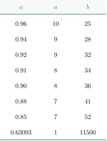
α a b

0.96 10 25

0.94 9 28

0.92 9 32

0.91 8 34

0.90 8 36

0.88 7 41

0.85 7 52

0.63093 1 11500

Table 2.1: This table shows that all possible exceptions to G(pα) >0 occur when

a≤ω(p−1)≤b.

3

Sieving

After the work of the previous chapter we are left with only a finite number of cases to check in order to prove Question 2.1 for variousα. Now in order to find a way to answer the question for these cases we need to understand why for these particular cases, the main term of (2.16) does not outweigh the error term.

The intervals in Table 2.1 are all for relatively small ω(p−1). To prove that

G(x) >0 for a particular case ofω(p−1), we have to prove it for allp ≥p0 where

p0 is the lower bound for p

p0 = max

2.5×1015,1 + 2·3· · ·5· · ·pω(p−1) .

When ω(p−1) is small then p0 is small and since the error term in (2.16)

decreases as p0 increases, we have that the main term is unable to outweigh the

error term. Now if there are some large primes dividingp−1 thenp0 will increase

which will decrease the error term in (2.16), making it more likely thatG(x)>0 for this particular case. Therefore if we can construct a version of G(x) that depends on the primes dividingp−1, then we should be able to prove Question 2.1 for more cases ofω(p−1).

In §3.2 of this chapter we will introduce the prime sieve which will result in a version of (2.16) that depends on the primes dividing p −1. This results in the reduction of cases left to prove. The prime sieve is frequently used to obtain results on the least primitive root modulo a prime. Not only was the sieve used in Cohen and Trudgian’s paper [6] on this topic, it was also used to prove Grosswald’s conjecture on the Generalised Riemann Hypothesis [21]. Theorem 2.1 was also proved using a version of the sieve as well as results on the sums of primitive roots [5] and consecutive primitive roots [4]. The following section §3.3 will outline how we will computationally reduce these cases even further. However first we need some background on e−free integers that is essential to defining the sieve.

3.1

e-free integers

Definition 3.1. Let pbe a prime and letebe a divisor of p−1. Supposep-nthen

nis e−freeif, for any divisor dof e, such that d >1,n≡yd (modp) is insoluble. Note that 2−free is not the same as square-free.

Definition 3.2. Let pi, where i = 1, . . . , ω(n) are the distinct prime divisors of n.

The radicalof nis

Rad(n) =p1p2· · ·pω(n).

The following proposition is important to the proof of Lemma 3.1, the indicator function for e−free integers. The proposition shows that the definition of e−free depends only on the distinct prime divisors of e. This proposition leads us to prove Proposition 3.2, which shows howe−free integers relate to primitive roots. Not only does Proposition 3.1 allow us to prove this important fact, it allows us to find the link between the prime divisors of p−1 and the error term of (2.16). This link is essential to the next step in answering Question 2.1 and will be outlined in§3.2.

Proposition 3.1. nis e−free ⇐⇒ n is Rad(e)−free. Proof. Let pbe a prime and let e|p−1.

Clearly e−free =⇒ Rad(e)−free as all divisors of Rad(e) also divide eand are not equal to 1.

Now to prove that Rad(e)−free =⇒e−free assumen(indivisible byp) is Rad(e)−free. That is for allf |Rad(e), n≡xf (modp) is insoluble (wherex is arbitrary). Supposenis not e−free, then there exists d|ewithd >1 such that

Since d | e, there exists f | Rad(e) such that f | d, in particular there exists an integerasuch thatf a=d. Therefore,

n≡yd≡yf a ≡xf (modp), where x=ya.

This is a contradiction to the assumption thatnis Rad(e)−free.

Proposition 3.2. nis a primitive root modulo p ⇐⇒ nis (p−1)−free. Proof. Fixg a primitive root modulo p.

First we prove that ifn is (p−1)−free then nis a primitive root modulo p. Letn≡gk (modp) then by Remark 1.1 it suffices to show

nis (p−1)−free =⇒(k, p−1) = 1.

Assumen is (p−1)−free, that is n6≡yd (modp),for alld|p−1,withd >1. Suppose (k, p−1) 6= 1 in particular (k, d0) = D for some d0 | p−1. Then D |k

and D|d0, in particular there exists integer asuch thatk=aD. Therefore,

n≡gk≡gaD≡yD (mod p), wherey=ga.

However D | d0 and d0 | p−1 so D | p−1, this is a contradiction to n being

(p−1)−free. Therefore (k, p−1) = 1.

Next we prove that ifn is a primitive root modulop thenn is (p−1)−free. Assumen is a primitive root modulop thenn≡gk (modp) if and only if (k, p−1) = 1.

Suppose n is not (p−1)−free, then there exists d | p−1 with d > 1 such that

n≡yd (modp).

Since g is a primitive root modulo p, there exists a ∈ {1, . . . , p−1} such that

y≡ga_{(mod p), therefore}

n≡yd≡gad (modp).

Sinced|(p−1), (ad, p−1)6= 1 which is a contradiction tonbeing a primitive root modulop. Thereforenis (p−1)−free.

Now with these two propositions we are able to define an indicator function for

Lemma 3.1 (Lemma 2 from [21]). Let p be a prime and let ebe a divisor of p−1. Then

φ(e)

e

X

d|e µ(d)

φ(d) X

χ∈Γd

χ(n) =  



1 if nis e−free,

0 otherwise,

(3.1)

where Γd is the set of Dirichlet characters modulop of order d.

Proof. Fix ga primitive root modulo pand let indgn=v.

Now let χ(n)∈Γd then asχ(n) is multiplicative we have

χ(n) =χ(g)v =e2πikv/d wherek= 1, . . . , d and (k, d) = 1.

So the innermost sum of 3.1 becomes X

χ∈Γd

χ(n) = X

1≤k≤d

(k, d)=1

e2πikv/d. (3.2)

From Proposition 1.4 we have

X

t|(k, d)

µ(t) =  



1 if (k, d) = 1,

0 otherwise.

Using this property we can rewrite (3.2) as the following X

1≤k≤d

(k, d)=1

e2πikv/d = X

1≤k≤d t|(k, d)

µ(t)e2πikv/d.

Now since t |(k, d) we have t | k and t | d so there exists an integer a such that

k=at. Therefore X

1≤k≤d t|(k, d)

µ(t)e2πikv/d = X

1≤k≤d t|k, t|d

µ(t)e2πikv/d =X

t|d

µ(t) X

1≤at≤d

e2πiatv/d.

Hence

X

χ∈Γd

χ(n) =X

t|d µ(t)

d/t

X

a=1

e2πiatv/d.

Suppose d - tv then e2πiavt/d6= 1 for all a and so we can consider the following geometric series

d/t

X

a=1

We therefore have

d/t

X

a=1

Xa= X(1−X

d/t₎

1−X = 0 asX

d/t _=e2πivt/dd/t _{= 1.}

Now consider whend|tv thene2πiavt/d= 1 for all aand so

d/t

X

a=1

Xa= d

t.

Therefore

X

χ∈Γd

χ(n) =  

 P

t|dµ(t) d

t ifd|tv,

0 otherwise.

Let m = (d, v) d | tv and recall Remark 1.2 which states µ(ab) = µ(a)µ(b) when (a, b) = 1, asµ is multiplicative, andµ(ab) = 0 otherwise. Then

X

χ∈Γd

χ(n) =X

t|m µ

t· d m

m t =

X

t|m

(t,_md)=1

µ(t)µ

d m m t =µ d m m X

t|m

(t,_md)=1

µ(t)1

t.

Using the Euler product (Theorem 285 in [15]) we obtain X

χ∈Γd

χ(n) =µ

d m

mY

p|m p-md

1 +µ(p)

p +

µ(p2₎

p2 +

µ(p3₎

p3 +. . .

=µ d m mY

p|m p-md

1−1

p

.

Using Proposition 1.5 we obtain X

χ∈Γd

χ(n) =µ

d m

φ(d)

φ _md.

Consider the case wherenis e−free, we will show that (v, d) = 1 for alld|e. Suppose (v, d0) = D for some d0 | e, then D | v and D | d0. So there exists

some integer a such that v = aD and so n= (ga)D however D | d0 |e. This is a

contradiction to n being e−free. Hence when n is e−free, (v, d) = 1 for all d | e. For this case consider the following

X

d|e µ(d)

φ(d) X

χ∈Γd

χ(n) =X

d|e µ(d)

φ(d)

µ(d)φ(d)

φ(d)

=X

d|e µ(d)2

Sinceφ(d) andµ(d) are both multiplicative, the sum over the divisors is multiplica-tive in eand we obtain

X

d|e µ(d)2

φ(d) = 

 X

d|pα1 1

µ(d)2

φ(d) 

. . . 

 X

d|pαrr

µ(d)2

φ(d) 



wheree=pα1

1 p

α2

2 . . . pαrr is the prime decomposition of e. Sinceµ(pα) = 0 for α >1

and µ(pα) =−1 whenα= 1 X

d|e µ(d)2

φ(d) =

1 + 1

φ(p1)

. . .

1 + 1

φ(pr)

=Y

p|e

p p−1

.

Now by Proposition 1.5 we have X

d|e µ(d)

φ(d) X

χ∈Γd

χ(n) = e

φ(e).

Next consider the case whennis note−free, thenM = (e, v)>1. We may assume

eis square-free by 3.1. Then X

d|e µ(d)

φ(d) X

χ∈Γd

χ(n) =X

d|e

µ(d) µ

d M

1

φ _Md

!

=X

d|e M

X

k|M

µ(dk)µ(d)

φ(d)

=X

d|e M

µ(d)2

φ(d) X

k|M

µ(k) = 0.

The inner sum is zero for allM >1 (Proposition 1.4). Hence

φ(e)

e

X

d|e µ(d)

φ(d) X

χ∈Γd

χ(n) =  



1 ifnise−free,

0 otherwise.

Now that we have an indicator function for e−free integers, we can sum this over the square-free integers to obtain an expression for the number of square-free and e−free integers. Given xand prime psuch thatx < p, letN_e2(p, x) denote the number of square-free and e−free integers less than x. Then from Proposition 3.2 we have N2(p, x) = N_p2₋₁(p, x). Now summing the indicator function for e−free integers (3.1) over the square-free integers less than x we have

N_e2(p, x) = φ(e)

e        X

n≤x n=2−free

1 +X

d|e d>1

µ(d)

φ(d) X

χ∈Γd

X

n≤x n=2−free

In the next section we will use (3.3) to obtain a sieving inequality. This inequality will enable us to define a sieving version ofG(x) (2.16). This will allow us to answer Question 2.1 for a number of the cases remaining from §2.1.

3.2

Results with sieving

The next step in answering Question 2.1 involves a sieving inequality, as mentioned above. In §2.1 the main term of (2.16) is unable to outweigh the error term for a fixed ω(p−1) when p is small. Therefore if there are some large primes dividing

p−1, p will be large and the main term is more likely to outweigh the error term, and our theorem will be proved for that specific case. The sieve uses this idea, by taking into account the primes dividingp−1.

Given prime p, let kbe a divisor of Rad(p−1). Then write

Rad(p−1) =kp1· · ·ps (3.4)

wherep1, . . . , ps are distinct primes with 1≤s≤ω(p−1) andk is the product of

the smallestω(p−1)−sdistinct primes dividing p−1. This is called sieving with corekandssieving primes. RecallN_e2(p, x) denote the number of integers less than

xthat are both square-free ande−free (givenp) and N2(p, x) denotes the number of square-free primitive roots modulo p less than x. The following lemma defines an inequality relating the number of square-free primitive roots with the number of square-free ande−free integers.

Lemma 3.2 (Lemma 2 from [6]). Given a prime p, assume that (3.4) holds. Then

N2(p, x)≥ s

X

i=1

N_kp2_i(p, x)−(s−1)N_k2(p, x) (3.5)

=

s

X

i=1

N_kp2_i(p, x)−

1− 1

pi

N_k2(p, x)

+δN_k2(p, x) (3.6)

where

δ= 1− s

X

i=1

1

pi

. (3.7)

Proof. Given n, a square-free and k−free integer, we will show that the right hand side of (3.5) contributes 1 if n is additionally pi−free for all i, and otherwise

con-tributes a non-positive quantity.

and (s−1) to (s−1)N_k2(p, x). Thereforencontributess−(s−1) = 1 to the right hand side of (3.5). Now Supposen is not additionally pi−free for all ithen it

con-tributesttoPs

i=1Nkp2i(p, x), where 0≤t < s and again (s−1) to (s−1)N

2 k(p, x).

In this casencontributest−(s−1) which is negative as t < s.

By the definition of e−free, if an integerx isk−free andpi−free, for alli, thenxis

Rad(p−1)−free. Furthermore by Proposition 3.1 x is (p−1)−free and therefore, by Proposition 3.2, xis a primitive root modulo p.

Hence for a square-free and k−free integern, if n is additionally pi−free then it is

a square-free primitive root modulop. Hence we obtain the inequality (3.5). Now to obtain (3.6) consider

s

X

i=1

N_kp2

i(p, x)−

1− 1

pi

N_k2(p, x)=

s

X

i=1

N_kp2

i(p, x)−sN

2

k(p, x) +Nk2(p, x) s X i=1 1 pi = s X i=1

N_kp2_i(p, x)−sN_k2(p, x) +N_k2(p, x)(1−δ)

=

s

X

i=1

N_kp2_i(p, x)−(s−1)N_k2(p, x)−δN_k2(p, x).

To find a lower bound on N_k2(p, x) we use the same method outlined in §2.1. Recall (2.13), the bound on the sum of Dirichlet characters, and (2.14), the lower bound for the number of square-free integers less than x. These bounds can be substituted into the indicator function (3.1) along with the number of square-free divisors ofk

X

d|k d>1

|µ(d)|= 2ω(k)−1

to obtain

N_k2≥ φ(k) k

x1/2p1/4

6

π2x

1/2_p−1/4₋0.104

p1/4 −

2ω(k)−1

E

. (3.8)

Recall

E ≤(logp)1/2

6

π2c

1/2_{(1 + ˆD) +}10

3 Ap

1/8−α/4_c3/4_(logp)1/4

.

A similar bound is found for each N_kp2

i wherei= 1, . . . , s and since

φ(kpi) kpi

= φ(k)

k

pi−1 pi

=

1− 1 pi

φ(k)

we have

N_kp2_i(p, x)−

1− 1

pi

N_k2(p, x) ≤ 1− 1

pi

φ(k)

k (x

1/2_p1/4₎n₂ω(kpi)₋₁

E−2ω(k)−1Eo

=

1− 1 pi

φ(k)

k (x

1/2_p1/4₎₂ω(kpi)₋₂ω(k)

E.

Sinceω(n) is the number of distinct prime factors of n

2ω(kpi)₋₂ω(pi)_{= 2}ω(k)+1₋₂ω(k)_{= 2}ω(k)₂₋₂ω(k) _{= 2}ω(k)_.

Therefore

N_kp2_i(p, x)−

1− 1

pi

N_k2(p, x) ≤ 1− 1

pi

φ(k)

k (x

1/2_p1/4₎₂ω(k)_{E. (3.9)}

The following theorem defines the sieving version of (2.16).

Theorem 3.1. Given the prime p, assume (3.4) holds. Let δ be given by (3.7).

Suppose δ >0 and let

∆ = s−1

δ + 2.

If

Gs(x) :=x1/2p−1/4− π2

6

0.104

p1/4 +

2ω(k)∆ + 1E

>0 (3.10) thenp has a square-free primitive root less than x.

Proof. Note

s

X

i=1

1− 1

pi

=s−

s

X

i=1

1

pi

=s−1 +δ.

Substituting (3.9) and (3.8) into Lemma 3.2 and using the above property we obtain

N2(p, x)≥ − s

X

i=1

1− 1 pi

φ(k)

k x

1/2_p1/4₂ω(k)_E

+δφ(k) k x

1/2_p1/4

6

π2x

1/2_p−1/4₋0.104

p1/4 −

2ω(k)−1E

=δφ(k) k x

1/2_p1/4

2ω(k)E

−1

δ(s−1 +δ)−1

+E+ 6

π2x

1/2_p−1/4₋0.104

p1/4

=δφ(k) k x

1/2_p1/4

2ω(k)E

−s−1 δ −2

+E+ 6

π2x

1/2_p−1/4₋ 0.104

p1/4

=δφ(k) k x

1/2_p1/4

6

π2x

1/2_p−1/4₋0.104

p1/4 −

2ω(k)∆ + 1E

ThereforeN2(p, x)>0 if

x1/2p−1/4−π

2

6

0.104

p1/4 +

2ω(k)∆ + 1E

>0.

Note thatGs(x) is very similar toG(x) from§2.1, however nowGs(x) depends on

the primes dividing p−1. The sieve was introduced because we needed G(pα)>0 for primes such that ω(p−1) is small. As we discussed in the beginning of this section, if there are some large primes dividing p−1 thenp0 will increase, for fixed

n= ω(p−1), and the error term in (2.16) will decrease. The error term in (3.10) depends on δ which in turn depends on the primes dividing p−1. The primes dividingp−1 affect the error term just as we expect: if there are some large primes dividingp−1 thenδ will increase, this results in the error term of (3.10) decreasing. This means for that particular case the main term is more likely to out weigh the error term.

Note that for any particular case ω(p−1) = n, we can choose the number of sieving primes, s. That is, we can choose s, for a fixed n, that minimises the error term in (3.10). At first one might think that we should just choose s = ω(p−1) because then we are including all primes inδ and 2ω(k) will be minimised. However

δ >0 and also the numerator of ∆ would be maximised. So choosing s=ω(p−1) will not necessarily minimise the error term. To find the right balance between k

and sfor a fixednthe optimal value of sis chosen such that it minimises the error term in (3.10).

To prove Question 2.1 withα= 0.9 the cases left to check are 8≤ω(p−1)≤36. Consider the first case,ω(p−1) = 8. We can find the optimals by calculating the error term from (3.10) for each 1 ≤ s ≤ 8 and selecting the s that generates the smallest error term. For this case s= 6 is optimal. As described above we would like δ to be large and so the worst case is if k = 2·3 and the sieving primes are the next 6 smallest primes. For this case δ ≥ 1−(5−1 _{+ 7}−1 _{+· · ·+p}−1

8 ). Now

substitutingδ, s= 6, x=p0.9 andω(k) = 2 into (3.10) shows for ω(p−1) = 8

Gs(p0.9)>0 for allp >1.42×1013.

Next consider the last case, ω(p−1) = 36. The optimalsfor this case is 32 and sok= 2·3·5·7 andδ≥1−(11−1+ 13−1+· · ·+p−₃₆1). Substitutingδ, s= 32 and

ω(k) = 4 into (3.10) shows that

Gs(p0.9)>0 for allp >2.98×1020.

Sinceω(p−1) = 36,p≥1 + 2·3·5· · ·p36= 2.25×1059. Therefore Question 2.1 with

α = 0.9 is also true for ω(p−1) = 36. Continuing in this way for each remaining case, 9≤ω(p−1)≤35, determining the optimalsand using it to find when (3.10) is true, we can prove Question 2.1 withα= 0.9 for all cases except ω(p−1) = 13.

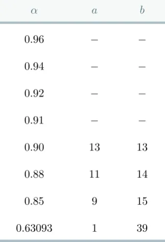
Table 3.1 shows the cases of Question 2.1 that cannot be answered at this stage. Compared to Table 2.1 we can see the improvement that the sieved equation makes. By using Theorem 3.1 we have significantly decreased the number of cases left to answer Question 2.1. For the lower bound on the exponent α we have gone from 11500 cases ofω(p−1) left to prove at the end of§2.1 to just 39 cases left to prove. Equivalently we have proved the following,

g2(p)< p0.63093 for all p >9.63×1065.

We have also shown that without the computational algorithm outlined in the next section we can prove the following.

All primes p have a primitive root less than p0.91.

α a b

0.96 − −

0.94 − −

0.92 − −

0.91 − −

0.90 13 13

0.88 11 14

0.85 9 15

0.63093 1 39

Table 3.1: This table shows that all possible exceptions to Gs(pα)>0 occur when a≤ω(p−1)≤b.

3.3

Results using the prime divisor tree

This section outlines the final step in our proof of Question 2.1. As explained above Theorem 3.1 depends on the primes dividing p−1. If there are some large primes dividingp−1 thenδ will increase and in turn the error term in (3.10) will decrease. Therefore we would like to take advantage of when there are some large primes dividingp−1. To do this we divide each case of ω(p−1) into sub cases depending on the primes dividingp−1. We can do this using an algorithm that works through a prime divisor tree.

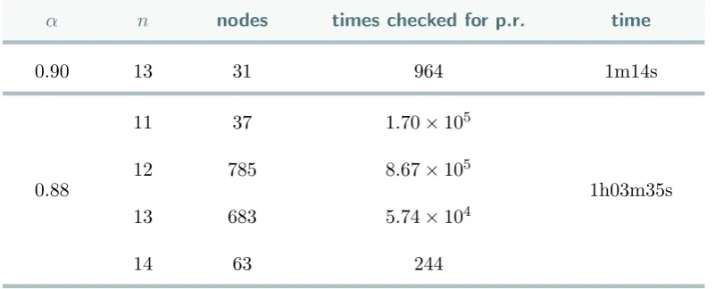
For example consider the caseα= 0.9 andω(p−1) = 13. After the second step in our proof, described in§3.2, we have that all possible exceptions for Question 2.1 to be true occur when p∈[2.5×1015,4.17×1015].

Since we know that 2 divides p−1 this is our base case (or base node) with the above interval of possible exceptions. The base node has s= 10 and therefore

δ≥1−(7−1+ 11−1+· · ·+p−₁₃1) = 0.416.

Now we look at the next level of our tree which has two nodes, when 3 |p−1 and when 3-p−1. First consider the case when 3 -p−1. Choosings= 10 gives