Remote sensing of extra equatorial planetary waves

Remote sensing of extra-equatorial planetary waves

in the oceans

Paolo Cipollini, Graham D. Quartly, Peter G. Challenor, David

Cromwell and Ian S. Robinson

Laboratory for Satellite Oceanography, Southampton

Oceanography Centre, U. K.

A contribution to Manual of Remote Sensing

Revision 05/04/2004

Corresponding author:

Dr. Paolo Cipollini

Room 254/30, Southampton Oceanography Centre

European Way, SO14 3ZH Southampton, United Kingdom

Remote sensing of extra-equatorial planetary waves in the

oceans

Waves in the ocean exist on a wide variety of spatial and temporal scales. A particularly interesting and important type is planetary waves, which are large-scale (hundreds to thousands of kilometres wavelength) perturbations of the ocean interior, with a surface signature of only a few centimetres amplitude. Their existence, due to the shape and rotation of the earth, was first predicted at the end of the 19th century, but nearly 100 years passed before it was realised that they were present throughout the ocean and could play a major role in maintaining and/or changing western boundary currents. The justification behind the study of these waves not only resides in their fascinating properties and in the fact that their detection has been a success story for marine remote sensing in recent years, but also, and more significantly, in their paramount importance for ocean circulation and climate, as will be clarified in the following.

The analysis presented in this section is restricted to extra-equatorial planetary waves because in the equatorial band the ocean dynamics results in propagating phenomena with generally longer spatial scales and faster speeds than their counterparts at mid-latitude (see below for further details). These equatorial waves are in some cases difficult to observe in satellite data (as the data may lack the necessary time resolution) or may require different analytical techniques for their identification, and will not be dealt with here.

1. Theory and properties of planetary waves

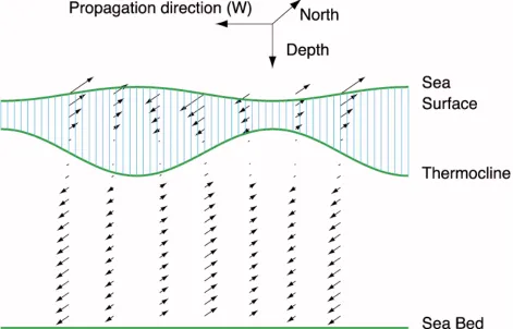
quantity akin to the parcel's angular momentum about the Earth's axis) provides a restoring force. Since the restoring force is proportional to the displacement the result is a sinusoidal signal, an intriguing property of which is that the propagation is westward, although the displacements are meridional (see Fig. 1).

Hough (1897) was the first to formulate the equations for planetary wave motion on a rotating sphere and discussed the solutions in spherical coordinates. Rossby et al. (1939) and Rossby (1940) approximated the problem into Cartesian coordinates on the so-called ‘-plane’. They did this by assuming that the Coriolis parameter f =2sin, where is the rotation rate of the earth (7.29 x 10-5

rad/s) and is the latitude, varies linearly with latitude, and could thus be written as f = f0+y where y is the meridional (north-south) coordinate and =f y. Those papers identified patterns of planetary waves in the atmosphere. In virtue of Carl-Gustav Rossby’s essential contribution to the subject, planetary waves are also widely known as Rossby waves. As stated in the introduction to this section, in the vicinity of the equator ( f 0) the equations for large-scale motion have to be solved with different approximations from the extra-equatorial case, and the dynamics of planetary and gravity waves become inter-related (see for instance chapter 8.5 of Pedlosky (1987)). In the following, therefore, the discussion will be restricted to extra-equatorial Rossby waves outside the 5°S-5°N latitude band, but for the sake of brevity they will be referred to simply as planetary waves here.

The low-frequency propagating solutions of the planetary wave equations outside the equatorial band are classically obtained with a further linearization about a state of zero background flow. These solutions can be cast on a number of orthogonal vertical modes with different depth structures identified by a mode number n. The mode with n=0 is depth-invariant and is called the barotropic mode. Modes with n>0 are depth-varying and called the baroclinic modes (the complete terminology is ‘first baroclinic’ for n=1, ‘second baroclinic’ for n=2, and so on). The speed of the modes is given by the so-called dispersion relationship, i.e. the relationship linking frequency and wavenumber of the mode. For propagating solutions of the form ~ exp

{

}

can be written as:

cnx = n

k = k2

+l2 +n

This provides the westward zonal phase speed cnx where n is the mode number, k, l are the

zonal (east-west) and meridional (north-south) wavenumbers, _n is frequency and n is a

characteristic length scale in the oceans known as the Rossby radius of deformation for mode

n. Equation (1) is a reasonable approximation throughout the deep ocean where friction

effects and nonlinear advection are negligible. The Rossby radius n depends on density

stratification and on 1 f . Updated global maps of 0 and 1 from historic hydrographic data

can be found in Chelton et al. (1998); 1is typically a few tens of kilometres at mid-latitudes.

The barotropic mode travels at many metres per second, traversing ocean basins in a matter of

weeks, often too fast to be resolved by satellites, so this will not concern us. However, there is

a great deal of interest in the much slower baroclinicmodes, especially the first baroclinic

mode, depicted in figure 1. The baroclinic modes travel at speeds of the order of 1-10 cm/s

(the higher the mode number, the slower the speed) and can affect the western boundary

currents, and thus have major repercussions on climate.

The minus sign on the right hand side of eq. (1) indicates that the zonal phase speed of

planetary waves is always westward: this is a consequence of the direction of the Earth’s

rotation. The meridional speed of the waves is usually negligible, i.e. they tend to propagate

westward or quasi-westward. Their wavelength is typically of hundreds or thousands of

kilometres, so they can be considered ‘long’ with respect to the Rossby radius, that is

k,l<<1 n

2

; as a consequence, c_nx=n 2

and the waves can also be regarded as

non-dispersive. The speed in that case varies with latitude approximately as cos sin2 (see the

solid line in the upper panel of figure 2). It can be demonstrated that in the long-wave

approximation both the phase and group velocities (group velocity is the velocity at which

pulses or "wave packets", made up of a range of different spectral components, travel) are

exactly westward, and that there exists a polewards latitude limit (called turning latitude)

beyond which planetary wave solutions become evanescent, i.e. no propagation exists (see

Gill (1982), pp. 440-443 for further details). For example, annual cycle baroclinic waves can

only exist for latitudes less than about 45°.

The importance attached to baroclinic planetary waves in modern oceanography stems from

multiple reasons: not only can they be regarded as the key response of the oceans to

large-scale changes in atmospheric forcing, and as the only means (other than boundary waves) by

which information is transferred from the eastern ocean boundaries to the west (e.g. Gill,

Current and the Gulf Stream, and, indeed, maintain these currents. Under particular

circumstances, planetary waves can even be responsible for disturbing the position of the

western boundary currents. For instance, Jacobs et al. (1994) present evidence for the

existence of an extra-tropical Rossby wave in the North Pacific, generated by the El Niño

event of 1982-83, and suggest that after a decade’s delay this wave induced a shifting of the

Kuroshio Current in the north-west Pacific. This shift may have affected the climate of North

America, and been responsible for the dramatic meteorological events in North America in

1993, such as the Mississippi flooding (McPhaden, 1994). In short, as well as being one of the

ways the ocean itself responds to climate events, Rossby waves may also delay the effects of

these events and control the dynamics of climate change and weather variability.

2. Altimetric observations of planetary waves

2.1 Historical notes

The important properties outlined in §1 have stimulated research on the occurrence,

distribution and generation mechanism of planetary waves in the oceans, as well as on their

properties, first and foremost their speed. But for many decades oceanographers found

themselves in the uncomfortable position of having an accepted theory for the phenomenon

but very scarce observational evidence for it, due to the inherent difficulties in measuring

planetary waves in situ, mainly because of the sheer difference in the wave horizontal and

vertical scales. Despite those difficulties, early proof of the occurrence of baroclinic planetary

waves in the ocean, namely variations in the depths of subsurface isotherms, was reported by,

amongst others, Emery and Magaard (1976) and White (1977). Over the next few years, a

sizeable body of evidence was built up, demonstrating the existence of Rossby waves in the

North Pacific ocean, in particular (see §3.4 of Fu and Chelton, 2001, for a full review of the in

situ observations). These pioneering studies indeed confirmed the existence of planetary

waves in the oceans, but due to the limitations of sampling could not provide the desired

characterization of the wave distributions and properties.

In more recent years, satellite altimeters have given indisputable confirmation of the

quasi-ubiquitous presence of planetary waves in the oceans. An earth-orbiting altimeter is in

principle capable of detecting their surface signature as westward propagating features in

characteristics (speed, wavelength, period) possible. It should be kept in mind that the surface

signature of the waves depends on integral properties of the whole water column; in the

illustration of a first-mode baroclinic wave shown in figure 1 the surface mirrors (with

amplitude reduced by about three orders of magnitude) the undulations of the thermocline

(the thermocline, sited at the bottom of the surface mixed layer, is a region of relatively strong

temperature and density change).

For the altimetric measurements of SSHA to be useful in practice, the following conditions

need to occur:

a) The accuracy of the SSHA field must be enough to detect signals of just a few cm,

which is the typical planetary wave amplitude;

b) The spatio-temporal sampling pattern of the altimeter and the length of the time series

are appropriate to resolve the phenomenon;

c) Other causes of SSHA variability can be identified and filtered out from the data. This

in turn requires that the relevant phenomena have typical spatial and temporal scales

distinguishable from those of planetary waves and that the sampling characteristics of

the altimeter do not alias those signals in a way that they might be misinterpreted as

planetary waves (see Parke et al. (1998) for a general discussion on aliasing problems

in altimeter data).

Of the first two altimetric missions, GEOS-3 lacked the necessary accuracy (condition a) and

SeaSat the time duration (b). The first direct altimetric observations of baroclinic planetary

waves thus were in the Geosat dataset (for instance White et al, 1990; Jacobs et al., 1992,

1993; Le Traon and Minster, 1993; Tokmakian and Challenor, 1993). Unfortunately, Geosat

suffered in respect to condition c): its 17-day repeat pattern meant that any residual M2 tidal

signal (tide not completely removed from the SSHA data – see the relevant chapter) would be

aliased at frequencies comparable with those of planetary waves, confusing the interpretation

of the results. However these pioneering studies firmly established the use of tools such as the

longitude/time plot and the relevant frequency/wavenumber diagram as the most natural

approach to investigate planetary wave propagation in satellite data – what was clear at the

time was that new spaceborne instruments were needed, with orbits designed to avoid the

The launch of TOPEX/POSEIDON (T/P) in 1992 marked the start of a new era in the

observations of planetary waves from space. Its 10-day repeat orbit pattern was specifically

selected to avoid tidal aliasing into frequencies of large–scale oceanic variability. Early T/P

studies identified planetary waves in various regions of the world’s oceans (Nerem et al,

1994, Wang and Koblinsky, 1995, 1996) but it was the global study of Chelton and Schlax

(1996) which demonstrated the ubiquity of the waves and showed that at mid-latitude they

tend to propagate faster than predicted by the linear theory (that is, faster than the speed given

by eq. 1 in the l=0 approximation, using atlases of 1based on historical hydrographic data).

A number of theories have been proposed in the attempt to reduce the discrepancy in speed;

the one yielding the most promising results to date is the extended theory by Killworth et al.

(1997) which, by including the effects of the baroclinic background mean flow, more closely

approaches the observed speed. Killworth et al.’s theory has been further extended or clarified

by Dewar (1998), Liu (1999), de Szoeke and Chelton (1999), and Killworth and Blundell

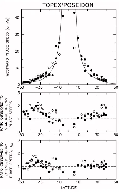
(1999, 2003a, 2003b). Figure 2, taken from Fu and Chelton, 2001, shows an updated version

of the speeds measured by Chelton and Schlax (1996), as well as the ratios of the speeds to

the prediction of the linear theory and the extended theory by Killworth et al. (1997). The

discrepancy between the observed speed and the linear theory speeds is apparent in the upper

and middle panel; the adoption of the extended theory greatly reduces this discrepancy as

shown in the bottom panel (a residual underestimation of the speed remains at mid-latitudes

in the southern hemisphere). A number of studies using altimeter data have contributed to

map the characteristics of the waves, including Polito and Cornillon (1997) and the recent

papers by Polito and Liu (2003), Fu (2004) and Osychnny and Cornillon (2004).

2.2 Techniques

This subsection discusses some processing techniques for the study of planetary waves in

altimetric and other satellite data. In view of the wave’s substantially east-west propagation,

initially the focus will be on the techniques used to observe the zonal characteristics for mode

n (zonal speed cnx, zonal wavelength 1/k and frequency ). As said in §2.1, the usual

approach for such an analysis is to build a particular kind of space-time diagram, called a

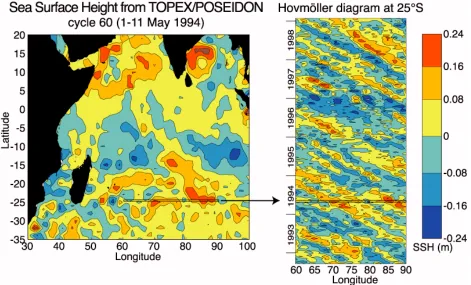
longitude-time plot or Hovmöller diagram. This can be easily obtained by taking, for each

time step, a section of data (SSHAs) at a given latitude and stacking all the sections from

different cycles, as exemplified in figure 3 for 25°S in the Indian Ocean. The time step of the

waves appear clearly in the plot as diagonal alignments: positive anomalies (‘crests’) and

negative anomalies (‘troughs’) that travel westward with time. Those in figure 3 have fairly

constant speed, but variations are possible in some locations; those will be discussed later.

Although some of the characteristics of the propagating waves in a longitude/time plot

can be approximately measured by eye (for instance, the speed is inversely proportional to the

slope of the alignments and could be roughly estimated by fitting a ruler to the plot itself),

more objective methods are needed. A number of two-dimensional data processing techniques

lend themselves to this purpose. The two most common ones, that is the two-dimensional

Fourier Transform (2D-FT) and Radon Transform (2D-RT), will be described in the

following subsections. Both these transforms map the longitude/time plot onto a transformed

space, that is the wavenumber/frequency (WF) space for the FT and a hybrid

velocity/projected coordinate space for the RT.

2.2.1 Use of the Fourier Transform

In practice, the 2D-FT of longitude time plots is implemented with the Fast Fourier

Transform algorithm (2D-FFT). It highlights the different spectral components of the plots,

which appear as peaks in the transform or spectrum in the WF domain. The 2D-FT is a

straightforward extension of the one-dimensional Fourier Transform (for more details on

general Fourier transform theory and FFT see Brigham (1988)). For an image s(mx,ny) of

M x N pixels, where m, n are the pixel indices and x,y the resolutions (pixel dimensions)

in the x and y directions, the 2D-FT is given by

S(f_x,f_y)=xy s(mx,ny)ej2(fxx+fyy) n=1 N

and in any practical implementation (including the 2D-FFT algorithm) it is computed on

a discrete grid

S(pfx,qfy), p=1KM, q=1KN with frequency (or wavenumber)

resolutions fx =1 (Mx) and fy=1 (Ny). S is periodic in both the fx and fy directions,

with periods 1x and 1y, and is generally complex, showing both the amplitude and phase

along x and time along y, the transformed fy axis corresponds to frequency proper (that is the

inverse of time) and fx to wavenumber (that is the inverse of space). Details on the 2D-FT and

other transforms for image analysis can be found in Jain (1989).

The 2D-FFT has long been used for the processing of altimetric data in the literature

(Le Traon and Minster, 1993, Tokmakian and Challenor, 1993); one of its advantages is that

it allows the detection of the single components of the propagating signals, which stand out as

peaks in the WF space and may correspond to the different baroclinic modes as suggested by

Cipollini et al. (1997) at 34°N in the North Atlantic and also observed by Subrahmanyam et

al. (1998) in the tropical Indian Ocean.

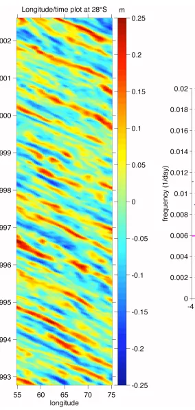
An example of application of the 2D-FFT is shown in figure 4. Figure 4a displays the

longitude/time plot, at latitude 28°S, longitude 55°E to 75°E in the Indian Ocean from

weekly, 1/3° SSHA data (data used for figures 4 to 7 are the DUACS merged T/P and ERS

SSHAs produced by the CLS Space Oceanography Division) spanning the period from

mid-October 1992 to early August 2002, for a total of 513 weeks. In the plot, the seasonal cycle

has been removed or filtered out by subtracting from each row the mean value of that row (a

more general 2D filtering technique will be briefly described later). Propagating planetary

waves are apparent in the plot. Their speeds show some degree of variability: for instance, by

eye it is possible to estimate that the negative anomaly around 75°E at the beginning of 1993

travels the whole longitude span (20°, corresponding to about 2000 km at this latitude) in

about 450 days, resulting in a speed of about 5.1 cm/s, while the positive anomaly entering

the plot from the east around April 1996 takes about 13 months to traverse the plot, giving a

speed of about 5.9 cm/s. Figure 4b shows the FFT of the data shown in fig. 4a. The

2D-FFT has three main peaks, corresponding to signals that propagate in the plot with speeds

between 5.5 and 6.4 cm/s. The peak marked as P3, with a wavelength of ~650 km and a

period of ~133 days, corresponds to a first-mode baroclinic Rossby wave propagating at a

speed of ~5.7 cm/s. This speed is slightly higher than the average speed of 4.7 cm/s predicted

by the extended theory of Killworth et al. (1997) over the same area, indicated by the dashed

between ~1000 and ~500 km, and speeds between ~7.2 and 4.0 cm/s, respectively, are

components that can be most readily identified looking at the relatively smaller-scale,

successive crests or troughs on the longitude/time plot itself. The other two major peaks, P1

(at the annual frequency) and P2 have longer wavelengths and periods but their speeds (6.4

cm/s and 5.5 cm/s, respectively) are within ±15% of the speed of P3, so it is not clear whether

these may represent different propagation modes. In other cases, the peaks are at very

different speeds from each other (such as the three signals at 3, 1.9 and 0.9 cm/s found at

34°N in the North Atlantic by Cipollini et al, 1997), and clearly indicate different modes of

propagation. Figure 4b also shows the dispersion curve (1) from Rossby’s linear theory

(magenta line), computed with the average value of 1 over the area, taken from Chelton et al.

(1998), that is 1=42.9 km; it can be noticed that all the peaks are above the curve, indicating

that the speeds of the relevant components are faster than the linear theory ones, whereas

there is much better agreement with the speed predicted by the extended theory of Killworth

et al. (1997).

A major drawback of the 2D-FT method (and also of the RT, see below) is that in order to

have distinct peaks in the spectrum, it must be applied to a portion of the data on a space and

time sub-domain where the propagation characteristics do not vary too much. On the other

hand, the resolution in the WF spectrum is inversely proportional to the width of the longitude

and time intervals used. If the interval is too narrow, adjacent peaks will be indistinguishable

from each other, so the selection of the sub-domain is a trade-off between resolution and

homogeneity. Moreover the FFT is well suited for the study of waves which appear to be

periodic in the space/time domain, and not appropriate for the study of single waves, such as

the one observed by Jacobs et al. (1994) in the Pacific as a result of the 1982-83 El Niño.

2.2.2 Use of the Radon Transform

When the focus of the analysis is on the propagation speed rather than on the wavelength and

period characteristics of the single components, the Radon Transform, first described by

Radon (1917) and whose properties are described in Deans (1983), is more appropriate. The

2D-RT p(x ,) at a given angle is the projection of an image (the longitude/time plot)

p(x ,)= f(x,y)

y

x=x cos y sin y=x sin+y cos

dy

The RT of a longitude/time plot, computed for two different angles 1 and 2, is shown in

Figure 5. FT and RT are related by means of the Projection-Slice theorem: p(x ,) is equal to

the inverse FT of a slice taken at the same angle in the Fourier space. This is important as

the lines at an angle , both in the longitude-time space and in the WF space, are lines of

constant speed, which can be readily computed from by simple trigonometric

considerations. Thus, computing the RT of the longitude-time plot for different values of ,

and then its energy, is equivalent to computing the energy in the spectrum along lines of

constant speed, and it is the most straightforward method to find the value of the speed for

which that energy is maximum. In other words, it is a method that yields an objective estimate

of the speed of the predominant propagating signal. To accomplish this, one needs to compute

the RT energy (i.e., sum the squares of the RT) for every , and find the value max for which

that energy is maximum (in figure 5 that angle is max=1, which is orthogonal to the dominant

direction of the alignments in the plot). The main propagation speed is then proportional to

the tangent of max. An application of the Radon Transform to find the speed of planetary

wave propagation in longitude/time plots of sea surface temperature (SST) data from the

Along-Track Scanning Radiometer (ATSR) on board the ERS-1 satellite has been described

in detail by Hill et al., (2000). The fundamental steps in Hill et al.’s method, with some

modifications, are described below, with reference to the longitude/time plot in figure 4a:

1. The longitude-time plot is pre-conditioned removing any outliers, filling any residual

gaps (missing values due, for instance, to cloud coverage in SST data or to islands)

with some form of interpolation and removing the mean of each row (fig. 4a includes

this step already);

2. The window may then be filtered with a 2-D filter, for instance one designed to

remove the high frequency noise or any variability at scales much smaller or much

larger that those of Rossby waves. Different filter designs can be adopted, including

local anomaly filters, various ‘band-pass’ filters to remove both very low frequency

variability and the high frequency noise or a ‘westward-only’ filter like the one

described in Cipollini et al., 2001, which highlights the westward propagating signals.

and third quadrants of the WF space (those being the westward-propagating

components) and zero response in the 2nd

and 4th

quadrant in WF space (including the

axes), has been used here to filter the longitude/time plot in figure 4a. This filter

leaves the westward propagating signals untouched and completely rejects any

stationary or eastward propagating one. The ‘westward-only’ filtered longitude-time

plot is shown in figure 6a;

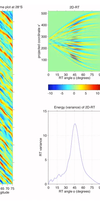
3. The Radon transform is performed for varying from 0° to 90° in steps of 1°, and its

energy or variance is computed for each . The transform and its variance are shown

in figures 6b and 6c, respectively;

4. The values of in the local maximaof the standard deviation are orthogonal to the

orientation of the alignments in the longitude-time plot, and thus can be converted into

an objective measure of the speed of propagation. These maxima can be identified

automatically, converted into propagation speeds and saved. A set of lines at an angle

normal to max=46°, that is normal to the angle of the large maximum in figure 6c, has

been drawn over Figure 6a for reference (these lines correspond to a propagation

speed of 5.6 cm/s). It is obvious that the broad peak in fig. 6c encompasses the

planetary waves in the original longitude/time plot; its width is a measure of the

spread in the speeds

Additional screening of the results is possible on the basis of the relative height of the peak in

the RT standard deviation plot, as performed in the SST analysis by Hill et al. (2000), or on

the basis of theoretical predictions as in the global example below.

The RT as described above can be easily automated and applied to longitude/time windows

moving over the whole globe.Figure 7a shows the result of the 2D-RT analysis of subsets of

merged T/P and ERS data of 20° longitude x 513 weeks centered at each integer latitude

value and every 2° longitude in the oceans. For each 2D-RT the angle of maximum energy

has been selected and the corresponding speed has been computed. The analysis has followed

points 1 to 4 above, with the addition of further screening of the peaks on the basis of the

speeds predicted by the extended theory by Killworth et al. (1997), recomputed using the newer climatologies in the World Ocean Atlas 1998 data (Antonov et al., 1998; Boyer et al.,

1998), which are shown in figure 7b. When the speed of the maximum peak was less than 1/3

peak has been selected instead, provided it passed the above criteria. Figure 7c shows the ratio

of fig. 7a and 7b, for ease of comparison.

The agreement between satellite-derived speeds and Killworth et al’s speeds is remarkably

good at latitudes between 15° and 35° in both hemispheres (where both are significantly

larger than those speeds estimated with the standard linear theory, as pointed out by Chelton

and Schlax (1996) and Killworth et al. (1997)). This is true especially in the Atlantic and

Indian Ocean, while in the Pacific, somewhat surprisingly, the observed speeds are almost

everywhere slightly slower than the extended theory ones. Conversely, in a band at higher

latitudes (approximately 35°N to 40°N in the North Atlantic, 30°S to 40S° in the Indian and

South Atlantic and up to 50°S in part of the South Pacific, there are patches where the

observed speeds can be up to 2-3 times larger that the extended theory ones. This is currently

being investigated.

Within 15°of the equator, the satellite-derived speeds are lower than both the linear theory

and the extended theory. There are two possible explanations for this:

1. The longitude span of 20° is too short to encompass the typical wavelengths of

planetary waves close to the equator,, resulting in aliasing of the wave characteristics

(a variable size longitude span should then be used, with some complications in the

processing).

2. In the tropics the 2D-RT preferentially picks up higher-order modes of propagation.

It is worth mentioning that the RT techniques just explained can be used for the study of

eastward phenomena in longitude/time plots of data (using a different range of ). It can also

be extended to the three-dimensional case in order to study the directional properties of

Rossby waves and estimate the meridional speed component in addition to the zonal one. A

description of the three-dimensional extension of the RT is presented in Challenor et al.

(2001). By applying this technique to T/P data in the North Atlantic, the same authors have

verified that in most locations the dominant propagating signal is within ±10° from pure

3 Observations in other remotely-sensed datasets

3.1 Observations in SST data and their meaning

As mentioned before, Hill et al. (2000) have found that the signature of planetary waves is

almost ubiquitous in global fields of SST measurements by the ATSR instrument (referenced

with respect to an in situ climatology). The SST-derived speeds computed by Hill et al agree

very well with the predictions of the extended theory by Killworth et al. (1997), apart form

some ‘slower than theory’ speeds at latitudes of 10-15° that might be due to the same reasons

outlined for the T/P observations.

SST observations of planetary waves are very important. While the thermal signature of the

waves may not be such a direct representation of their dynamical characteristics as is the SSH

signal, it must be pointed out that it is the thermal signature which is influential for the

processes of ocean-atmosphere interaction. The coupling between ocean and atmosphere can

be, in turn, responsible for changes in the planetary wave characteristics, as hypothesized by

White et al. (1998). In some cases simultaneous SST/SSH observations can provide additional

information on the modal structure of the waves (as in Cipollini et al., 1997) or even, in

conjunction with ocean colour data, on the mechanisms by which biology is affected by the

waves; this will be discussed in §3.3.

It should be noted that a promising class of instruments for this kind of observations are

passive microwave radiometers measuring SST. These measurements, whose relatively low

geometrical resolution (tens of km) is still more than enough for the observation of large-scale

phenomena, are unaffected by clouds and thus provide a good dataset to investigate planetary

waves. Quartly et al. (2003) have found evidence of planetary waves in the Indian Ocean in

data from the TMI on board TRMM and illustrate that with an example at 32°S. A similar

example is presented in §3.3.

3.2 Observations in ocean colour

Recently, evidence of propagating signals with speeds consistent with those of planetary

waves has been found in filtered longitude/time plots of phytoplankton chlorophyll

concentration from ocean colour radiometers (Cipollini et al., 2001, Uz et al., 2001). Figure 8,

the Indian Ocean after high-pass and westward-only filtering (see the relevant paper for more

details on the filters). A number of propagating anomalies are apparent in the plot. Their

speed can be evaluated with the 2D-RT technique described in §2.2, giving a peak at 3.7

cm/s. By comparison, the same analysis on T/P data in the same location gives a peak at 4.0

cm/s, within 10% of the ocean-colour result. The ocean-colour-derived speeds observed by

Cipollini et al. in various locations in the different ocean basins show a broad agreement with

the other satellite observations and the extended theory.

A number of possible mechanisms may be responsible for the presence of the planetary wave

signature in ocean colour data:

i. Advection of chlorophyll gradients - advection of meridional gradients of

phytoplankton due to the geostrophic currents associated with the passage of the

waves. In this case phytoplankton acts just as a passive tracer;

ii. Shoaling of the deep chlorophyll maximum - the modification of the isopycnals due to

the passage of a wave could bring more phytoplankton cells closer to the surface or

vice versa, and thus either affect the amount of phytoplankton seen by the satellite

without changing its total (vertically-integrated) amount (see Charria et al., 2003), or

increase/decrease growth, by bringing more cells into the euphotic zone or pushing

them out of it.

iii. Nutrient pumping effect - the modification in the upwelling of nutrients due to the

raising and lowering of the thermocline associated with a wave, and thus a direct

effect on the growth of a nutrient-limited population of cells. This is the so-called

‘rototiller effect’ (Siegel, 2001).

Understanding which mechanism predominates requires a careful intercomparison of the

signature of the waves in different datasets, as explained below. The effect of planetary waves

on biology could prove to be significant for studies of the global carbon cycle, especially if

the occurrence of mechanism iii above is proved. Very recently, Killworth et al (2004) have

carried out a global cross-spectral analysis of ocean colour and SSHA data and its comparison

with theoretical predictions from models of the mechanisms listed above. Their main finding

is that the horizontal advection of chlorophyll gradients is the main mechanisms over most of

the ocean, although it cannot be ruled out that there exist locations where additional biological

3.3 Synergy of planetary wave observations in different datasets

The following example illustrates how, by looking at the signature of the waves in different

datasets, and in particular at their phase relationship, it is possible to infer more information

about the underlying mechanisms of interaction between the waves and the SST and ocean

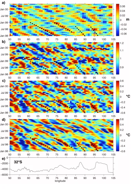
colour fields. Figure 9 shows data at 32°S in the Indian Ocean from 4 different sensors flying

on 4 different spacecraft: T/P SSHA, ocean colour data observed by SeaWiFS, SST from

ATSR-2 and another SST field, but derived from TMI, the passive microwave sensor on the

TRMM platform.

In figure 9 a spatial filter has been applied to each dataset in turn, to produce anomalies

relative to the local mean. All four parameters display westward-propagating features. The

signals are clearest in the SSH field, especially in the western half of the basin where the

alignments of crests and troughs run parallel (i.e. with the same propagation speed) and each

feature maintains approximately the same magnitude, albeit that the amplitude of separate

features can vary from as little as 2 cm to more than 6 cm. The signals in the western basin

have a wavelength of ~800 km, a period of ~7 months and a speed of ~4.4 cm/s. The

chlorophyll signature of Rossby waves is by no means as clear as in SSH. There is a strong

intra-annual variation; in the western half, the greatest proportional changes occurring around

September 1998 (at the peak of the bloom), whereas in the east the chlorophyll anomalies are

greatest in early 1999. However, within the limited extent of the time series it is not clear that

this is a seasonal modulation.

In subplots c) and d) in fig. 9, which show the SST anomalies from infra-red and passive

microwave sensors, it is very impressive just how well these two datasets agree — not just in

the timing of propagation features but in their magnitude too. It should be recalled that these

are two independent datasets using different technologies on different platforms. As the

principal errors for infrared SST measurements are due to thin clouds and those for

microwaves are due to wind speed and orientation, the retrieval errors for these two datasets

are totally independent. Of the two, the waves appear clearer in the TMI data — thus proving

the usefulness of TMI in monitoring large-scale features such as planetary waves. To ease the

comparison of the features, four straight dashed lines are overlaid in the same location in all

plots and have been positioned along some significant reductions in chlorophyll (Fig. 9b). The

indicate a higher-order propagation mode. Both of the slower features can be seen in the

ATSR-2 data, with one clear and the other just discernible in the TMI values too.

When looking at the phase relationship of these different signatures it can be seen that all four

lines demarking decreases in chlorophyll also lie close to local maxima in SST. However, the

westernmost two (first baroclinic modes) delineate the change from below average SSH to

above average i.e. the SSH signals lag the SST signature by approximately 90°, but lead the

ocean colour signature by a similar amount. The bathymetry might play an important part,

since there are significant ridges at 97°E and 87°E. In numerical models it has been noted that

rapid changes in bathymetry can cause the interchange of energy between different baroclinic

modes (Barnier, 1988).

In the southern hemisphere, the geostrophic velocities associated with the passage of a

planetary wave crest are directed as shown in figure 10. If a parameter has a positive

meridional gradient (shown schematically in fig. 10 as a front), which is the case for SST

there, then the signal due to the resulting advection of this gradient should lead the SSH signal

by approximately 90°, as shown in the bottom panel of figure 10. If, on the contrary, the

meridional gradient is negative (this happens for phytoplankton at 32°S, where moving

equatorwards there is a transition from the productive mid-latitude waters to the oligotrophic

waters at the interior of the subtropical gyre), then the signal resulting from advection should

trail the SSH signal by approximately 90°. This is what is observed for the data in figure 9. It

can be concluded that, in this location of the Indian Ocean, lateral displacement due to

advection is the predominant mechanism for the presence of an ocean colour and thermal

signature of planetary waves. In the discussion above, and in the schematics in figure 10, it

has been assumed that the advected tracer anomalies (chlorophyll or SST) decay and go back

to equilibrium (their background values) in a much shorter time than the wave period, so that

the displacement of the anomalies is approximately proportional to the instantaneous

geostrophic velocity rather than to its integral; the ‘decay’ time of the advected parameter is,

for instance, the time taken by SST to reach equilibrium with the overlaying atmosphere in

virtue of heat exchange, or the mean life time of a population of phytoplankton cells. If the

decay is comparable or longer than the wave period, the phase relationship changes, as

discussed in detail by Killworth et al., 2004.

Quartly et al. (2003) show a case study at 34˚S with similar results — chlorophyll decreases

with no clear SSHA signal for the slower modes. North of about 30˚S they note that the

cross-correlation of temperature and chlorophyll anomalies is positive. This partially reflects

the change in sign of the meridional chlorophyll gradient, however Quartly et al. (2003) note

that between 25˚ and 30˚S the gradient changes sign with the season, due to a strong

secondary bloom of phytoplankton in February-March (Longhurst, 2001). This secondary

bloom is only present for about half the years since 1997, covered by the SeaWiFS mission.

Eddy activity along 25°-27°S may help mediate the development of this bloom (Srokosz et

al., 2004) and could complicate the determination of the SSHA-chlorophyll phase relationship

of planetary waves in this particular region.

Killworth et al. (2004) have examined the cross-correlation between SSH and chlorophyll

concentration on a global basis, contrasting the observed phase relationship with that expected

for the different mechanisms listed in section 3.2. For mid-latitudes (both southern and

northern hemispheres) they show the phase difference between chlorophyll and SSHA signals

agree well with the predictions of the advection mechanism, indicating that advection plays

an important role. However there is less agreement on the amplitudes, the observed

chlorophyll signal being often larger than what would be expected from pure horizontal

advection. This could indicate the occurrence of vertical mechanisms, especially upwelling

which in theory could give large chlorophyll signals in several regions of the world ocean and

therefore could have an influence on primary production and the global carbon cycle. This

marks the current frontier in planetary wave research.

4. Summary

In 1897, Hough predicted the existence of long wavelength planetary waves, which

correspond to north-south oscillations of the water column, but with the direction of

propagation usually being close to due west. However, it was only in the 1990s that it was

realised that they were prevalent in all ocean basins (up to a limiting turning latitude). The

leap forward in observations, and consequently in theoretical studies, was due to the advent of

long-term consistent global satellite datasets of a high quality. Planetary waves are usually

most clearly seen in measurements of SSHA from spaceborne radar altimeters, despite the

surface variation only being a few centimetres rather than the tens of metres variation deeper

Transform — can be used to derive the key parameters of the wave, viz. wavelength, period

and speed. The latter is very important as it sets the response time of western boundary

currents to disturbances that have occurred at the east of the ocean. The observed westward

propagation speed is a few cm/sec (a few km/day) at mid-latitudes, and increases equatorward

as predicted by theory. However, the speeds predicted by the original theory underestimated

the true speeds by as much as a factor of two. Consequently there have been several revisions

to the theory to include the effects of currents and sloping bathymetry.

The near-global observations of planetary waves in SST and ocean colour are an even more

recent discovery, whose implications are not yet fully resolved. Assuming that SST and

chlorophyll concentration vary with latitude, planetary waves would be expected to generate

temperature and colour signatures through the simple north-south advection of water

associated with the waves. Recent research has confirmed that this horizontal mechanism is

certainly important, but some discrepancies between the observed and modelled signals,

especially in the amplitude relationships between chlorophyll and SSHAs signals, may

suggest that vertical mechanisms are at play in some regions. For instance, in some locations

the meridional gradient in chlorophyll is minimal, so the horizontal advection mechanism

could not explain the observed ocean colour signal in the first place, raising the prospect that

planetary waves may actually be promoting plankton growth there. Quantifying the effects of

planetary waves on the global carbon cycle, and the long-term variability of these effects, are

References

Antonov, J., Levitus, S., T. P. Boyer, M. Conkright, T. O’Brien, C. Stephens, 1998: World

Ocean Atlas 1998 Vols. 1-3: Temperature of the Atlantic/Pacific/Indian Ocean. NOAA

Atlas NESDIS 27. U.S. Gov. Printing Office, Wash., D.C., 166 pp.

Barnier B., A numerical study on the influence of the Mid-Atlantic Ridge on nonlinear

first-mode baroclinic Rossby waves generated by seasonal winds, J. Phys. Oceanogr., 18,

417-433, 1988.

Boyer, T. P., Levitus, S., J. Antonov, M. Conkright, T. O’Brien, and C. Stephens, 1998:

World Ocean Atlas 1998 Vols. 4-6: Salinity of the Atlantic/Pacific/Indian Ocean.

NOAA Atlas NESDIS 30. U.S. Gov. Printing Office, Wash., D.C., 166 pp.

Brigham, E. O., The Fast Fourier Transform and its applications, 448 pp., Prentice Hall,

1988.

Challenor, P. G., P. Cipollini, D. Cromwell, Use of the 3-D Radon Transform to examine the

properties of oceanic Rossby waves, J. Atmosph. Ocean. Tech., vol. 18, no. 9, pp.

1558-1566, 2001. See also: Corrigendum, J. Atmosph. Ocean. Tech., vol. 19, no. 5, p. 828,

2002.

Charria, G., F. Mélin, I. Dadou, M.-H. Radenac, and V. Garçon, 2003: Rossby wave and

ocean color: The cells uplifting hypothesis in the South Atlantic Subtropical

Convergence Zone. Geophys. Res. Lett., 30, 10.129/2002GL016390.

Chelton, D. B. and M. G. Schlax, Global observations of oceanic Rossby waves, Science, 272,

234-238, 1996.

Chelton, D. B., R. A. de Szoeke, M. G. Schlax, K. E. Naggar, and N. Siwertz, Geographical

variability of the first baroclinic Rossby radius of deformation, Journal of Physical

Cipollini, P., D. Cromwell, M. S. Jones, G. D. Quartly and P. G. Challenor, Concurrent

altimeter and infrared observations of Rossby wave propagation near 34° N in the

Northeast Atlantic, Geophysical Research Letters,. 24 ,. 889-892, 1997.

Cipollini, P., D. Cromwell, P. G. Challenor and S. Raffaglio, “Rossby waves detected in

global ocean colour data”, Geophysical Research Letters,. 28 , 323-326, 2001.

Deans, S.R., The Radon transform and some of its applications: John Wiley, 1983.

Dewar, W. K., 1998: On “too fast” baroclinic planetary waves in the general circulation. J.

Phys. Oceanogr., 28, 1739-1758.

de Szoeke, R. A., and D. B. Chelton, 1999: The modification of long planetary waves by

homogeneous potential vorticity layers. J. Phys. Oceanogr., 29, 500-511.

Emery, W. and L. Magaard, Baroclinic Rossby waves as inferred from temperature

fluctuation in the eastern Pacific, Journal of Marine Research 34: 365-385, 1976.

Fu, L.-L. and D. B. Chelton, Large Scale Ocean circulation, in Satellite Altimetry and Earth

sciences, eds. L.-L. Fu and A. Cazenave, Academic Press, 2001.

Fu, L.-L., Latitudinal and frequency characteristics of the westward propagation of largescale

oceanic variability, submitted to J. Phys. Oceanography, 2004.

Gill, A. E., Atmosphere-Ocean Dynamics, Academic Press, San Diego, 1982.

Hill, K. L., I. S. Robinson and P. Cipollini, “Propagation characteristics of extratropical

planetary waves observed in the ATSR global sea surface temperature record”, Journal

of Geophysical Research - Oceans, v. 105(C9), pp. 21,927-21.945, 2000.

Hough, S. On the application of harmonic analysis to the dynamical theory of the tides, Part I.

On Laplace’s ‘oscillations of the first species’, and on the dynamics of ocean currents.

Jacobs, G. A., H. E. Hurlburt, J. C. Kindle, E. J. Metzger, J. L. Mitchell, W. J. Teague, and A.

J. Wallcraft, Decade-scale trans-Pacific propagation and warming effects of an El Niño

anomaly, Nature, 370, 360-363, 1994.

Jacobs, G. A., Born, G. H., Parke, M. E., and Allen, P. C., The global structure of the annual

and semiannual sea surface height variability from Geosat altimeter data. J. Geophys.

Res., 97, 17,813-17,828, 1992.

Jacobs, G. A., W. J. Emery and G. H. Born, Rossby waves in the Pacific Ocean extracted

from Geosat altimeter data, J. Phys. Oceanogr., 23, 1155-1175, 1993.

Jain, A. K. , Fundamentals of Digital Image Processing, 569 pp., Prentice-Hall, 1989.

Killworth, P. D., and Blundell, J. R., The effect of bottom topography on the speed of long

extratropical planetary waves. J. Phys. Oceanogr., 29, 2689-2710, 1999.

Killworth, P. D. and J. R. Blundell, 2003a: Long extra-tropical planetary wave propagation in

the presence of slowly varying mean flow and bottom topography. I: the local problem.

J. Phys. Oceanogr., 33, 784-801.

Killworth, P. D. and J. R. Blundell, 2003b: Long extra-tropical planetary wave propagation in

the presence of slowly varying mean flow and bottom topography. II: ray propagation

and comparison with observations. J. Phys. Oceanogr., 33, 802-821.

Killworth, P. D., D. B. Chelton and R. de Szoeke, The speed of observed and theoretical long

extra-tropical planetary waves. J. Phys. Oceanogr., 27, 1946-1966, 1997.

Killworth, P. D., P. Cipollini, B. M. Uz and J. R. Blundell, Physical and biological

mechanisms for planetary waves observed in satellite-derived chlorophyll, J. Geophys.

Res., in press, 2004.

Le Traon, P.-Y. and J.-F. Minster, Sea Level Variability and Semiannual Rossby Waves in

Liu, Z., 1999: Forced planetary wave response in a thermocline gyre. J. Phys. Oceanogr., 29,

1036-1055.

Longhurst, A., A major seasonal phytoplankton bloom in the Madagascar Basin, Deep Sea

Research I, 48, 2413-2422, 2001.

McPhaden, M.J, The eleven-year El Niño?, Nature, 370, 326, 1994.

Nerem, R. S., Schrama, E. J., Koblinsky, C. J., and Beckley, B. D., A preliminary evaluation

of ocean topography from the TOPEX/POSEIDON mission. J. Geophys. Res., 99,

24,565-24,583, 1994.

Osychny, V. and P. Cornillon, Properties of Rossby Waves in the North Atlantic Estimated

from Satellite Data, J. Phys. Oceanography, 34, 61-76, 2004.

Parke, M.E., G. Born, R. Leben, C. McLaughlin and C. Tierney, Altimeter sampling

characteristics using a single satellite, J. Geophys. Res., 103, 10513-10526, 1998.

Pedlosky, J., Geophysical Fluid Dynamics. 2nd Ed., Springer-Verlag, 710 pp., 1987.

Polito, P. S., and P. Cornillon: Long baroclinic Rossby waves detected by

TOPEX/POSEIDON. J. Geophys. Res., 102, 3215– 3235, 1997.

Polito, P. S., and W. T. Liu, Global characterization of Rossby waves at several spectral

bands, J. Geophys. Res., 108(C1), 3018, doi:10.1029/2000JC000607, 2003.

Quartly, G. D., P. Cipollini, D. Cromwell and, P. G. Challenor, Rossby waves: Synergy in

action, Phil. Trans. Royal Society London A., 361 , 57-63, 2003.

Radon, J., Über die Bestimmung von Funktionen durch ihre Integralwerte längs gewisser

Mannigfaltigkeiten, Berichte Sächsische Akademie der Wissenschaften. Leipzig,

Math.–Phys. Kl., 69, 262-267, 1917. English translation in S.R. Deans, The Radon

transform and some of its applications: John Wiley, pp. 204-217, 1983.

Rossby, C. G., Planetary flow patterns in the atmosphere. Q. J. Roy. Meteor. Soc., 66, 68-87,

Rossby, C. G., and Collaborators, Relations between variations in the intensity of the zonal

circulation of the atmosphere and the displacements of the semi-permanent centers of

action. J. Mar. Res., 2, 38-55, 1939.

Siegel, D.A., The Rossby rototiller, Nature, v. 409, pp. 576-577, 2001.

Srokosz, M. A., G. D., Quartly and J. J. H. Buck, A possible plankton wave in the Indian

Ocean, submitted to Geophysical Research Letters, 2004.

Subrahmanyam, B., I. S. Robinson, J. R. Blundell and P. G. Challenor, Rossby waves in the

Indian Ocean from TOPEX/POSEIDON altimeter and model simulations, Int. J.

Remote Sensing, 2001.

Tokmakian, R. T. and P. G. Challenor, Observations in the Canary Basin and the Azores

Frontal Region Using Geosat Data, J. Geophys. Res., 98, 4761-4773, 1993.

Uz, B. M., Yoder, J. A. & Osychny, V. Pumping of nutrients to ocean surface waters by the

action of propagating planetary waves, Nature v. 409, pp. 597–600, 2001.

Wang, L., and Koblinsky, C. J., Low-frequency variability in regions of the Kuroshio

Extension and the Gulf Stream. J. Geophys. Res., 100, 18,313-18,331, 1995.

Wang, L., and Koblinsky, C. J., Low-frequency variability in the region of the Agulhas

Retroflection. J. Geophys. Res., 101, 3597-3614, 1996.

White, W. B., "Annual forcing of baroclinic long waves in the tropical North Pacific Ocean."

Journal of Physical Oceanography 7: 50-61, 1977.

White, W. B., Tai, C.-T., and DiMento, J., Annual Rossby wave characteristics in the

California Current region from the Geosat exact repeat mission. J. Phys. Oceanogr., 20,

1297-1311, 1990.

White, W. B., Chao, Y., and Tai, C.-K., Coupling of biennial oceanic Rossby waves with the

Figure Captions

Figure 1 – schematic of a first-mode baroclinic planetary wave in the northern hemisphere.

Figure 2 – (From Fu and Chelton, 2001). Upper panel: comparison between

TOPEX/POSEIDON measured speeds (circles) and the zonal average of speed predicted from

linear theory (solid line). Centre panel: ratio T/P-derived speeds vs linear theory. Lower

panel: ratio T/P-derived speeds vs Killworth et al.’s extended theory. Solid circles are for

locations in the Pacific, open circles for locations in the Atlantic and Indian (Note – copyright

clearance needs to be sought for this figure)

Figure 3 – Schematic of the production of a longitude/time plot

Figure 4 – a) Longitude/time plot of merged T/P and ERS SSHAs (m) at 28°S in the Indian

Ocean; b) Amplitude of the 2D-FFT of the longitude/time plot in a). The diagram has been

flipped horizontally so that westward-propagating signals are on the left quadrant. Contours

start from 100 m·degrees·days (dark blue contour) and increase in steps of 100

m·degrees·days. The approximate wavelength , period T and zonal speed cx of the peaks are:

P1 - 2000 km, T360 days, cx6.4 cm/s; P2 - 1000 km, T211 days, cx5.5 cm/s; P3

650 km, T133 days, cx5.7 cm/s; P4 - 1000 km, T164 days, cx7.1 cm/s; P5 - 650

km, T156 days, cx4.8 cm/s; P6 - 600 km, T143 days, cx4.9 cm/s; P7 - 500 km,

T124 days, cx4.0 cm/s. The magenta curve is eq. (1) with a Rossby radius of 42.9 km; the

red dashed line corresponds to a speed of 4.7 cm/s which is the median speed from the

extended theory of Killworth et al. (1997) over the area.

Figure 5 – Example of 2D Radon Transform of a longitude/time plot f(x,y) computed for two

different angles 1 and 2

Figure 6 – a) same longitude/time plot as in Fig. 4, after westward-only filtering as described

in the text. The superimposed solid lines have a slope corresponding to the speed of

maximum energy in the RT, that is 5.6 cm/s. b) 2D-RT of the longitude/time plot and c) its

standard deviation.

Figure 7 – a) Main zonal propagation speed from the 2D-RT analysis of longitude/time plots

theory by Killworth et al. (1997), recomputed using the climatologies in the World Ocean

Atlas 1998 data (Antonov et al., 1998; Boyer et al., 1998); c) ratio of a) to b).

Figure 8 – westward-propagating signals in a filtered longitude/time plot of Ocean colour

(OCTS + SeaWiFS) data – from Cipollini et al., 2001.

Figure 9 – Longitude/time plots of four different datasets at 32°S in the Indian Ocean, filtered

with a local anomaly filter. a) T/P SSHAs (m); b) chlorophyll concentration (expressed as

ratio to local mean) from SeaWiFS; c) SST from ATSR-2 (°C); d) SST from TMI (°C); e)

bathymetry.

Figure 10 – Mechanism of advection of meridional gradients by the geostrophic velocities

associated with planetary waves. The arrows indicate the geostrophic velocities. Note that in

the bottom panel it has been assumed that the ‘decay’ time of the advected parameter (for

instance, the time taken by SST to reach equilibrium with the overlaying atmosphere in virtue

of heat exchange, or the mean life time of a population of phytoplankton cells) is small with

respect to the wave period, so that the displacement is approximately proportional to the

instantaneous geostrophic velocity rather than to its integral (for more details on the effects of