This is a repository copy of
Analytical prediction of chatter stability for variable pitch and
variable helix milling tools
.
White Rose Research Online URL for this paper:
http://eprints.whiterose.ac.uk/8871/
Article:
Sims, N.D., Mann, B. and Huyanan, S. (2008) Analytical prediction of chatter stability for
variable pitch and variable helix milling tools. Journal of Sound and Vibration, 317 (3-5).
pp. 664-686. ISSN 0022-460X
https://doi.org/10.1016/j.jsv.2008.03.045
[email protected] https://eprints.whiterose.ac.uk/ Reuse
Unless indicated otherwise, fulltext items are protected by copyright with all rights reserved. The copyright exception in section 29 of the Copyright, Designs and Patents Act 1988 allows the making of a single copy solely for the purpose of non-commercial research or private study within the limits of fair dealing. The publisher or other rights-holder may allow further reproduction and re-use of this version - refer to the White Rose Research Online record for this item. Where records identify the publisher as the copyright holder, users can verify any specific terms of use on the publisher’s website.
Takedown
If you consider content in White Rose Research Online to be in breach of UK law, please notify us by
promoting access to White Rose research papers
White Rose Research Online
Universities of Leeds, Sheffield and York
http://eprints.whiterose.ac.uk/
This is an author produced version of a paper accepted for publication in Journal
of Sound and Vibration.
White Rose Research Online URL for this paper:
http://eprints.whiterose.ac.uk/8871/
Published paper
Sims, N.D., Mann, B. and Huyanan, S. (2008) Analytical prediction of chatter
stability for variable pitch and variable helix milling tools. Journal of Sound and
Vibration, 317 (3-5). pp. 664-686.
Analytical prediction of chatter stability for variable
pitch and variable helix milling tools
N D Sims
a, B Mann
b, and S Huyanan
a aDepartment of Mechanical Engineering
The University of Sheffield
Mappin St, Sheffield S1 3JD, UK
bDepartment of Mechanical Engineering & Materials Science
Duke University
Durham, NC 27708, USA
Abstract
Regenerative chatter is a self-excited vibration that can occur during milling and other
machining processes. It leads to a poor surface finish, premature tool wear, and potential
damage to the machine or tool. Variable pitch and variable helix milling tools have been
previously proposed to avoid the onset of regenerative chatter. Although variable pitch tools
have been considered in some detail in previous research, this has generally focussed on
behaviour at high radial immersions. In contrast there has been very little work focussed on
predicting the stability of variable helix tools. In the present study, three solution processes
are proposed for predicting the stability of variable pitch or helix milling tools.
The first is a semi-discretisation formulation that performs spatial and temporal discretisation
of the tool. Unlike previously published methods this can predict the stability of variable pitch
or variable helix tools, at low or high radial immersions.
The second is a time-averaged semi-discretisation formulation that assumes time-averaged
cutting force coefficients. Unlike previous work, this can predict stability of variable helix
tools at high radial immersion.
The third is a temporal-finite element formulation that can predict the stability of variable
pitch tools with a constant uniform helix angle, at low radial immersion.
Nomenclature
a
direction coefficient (subscripts x and y
denoting two directions)
a
average direction coefficient for 1 time step (subscripts x and y
denoting directions)
A
state matrix for the complete system
A
dstate matrix for the system delays
A
mstate matrix for the discretised structural dynamics
A
sstate matrix for the structural dynamics
A
tstate matrix for the time finite element analysis method
b
depth of cut (m)
B
input matrix for the complete system
B
dinput matrix for the system delays
B
minput matrix for the discretised structural dynamics
B
sinput matrix for the structural dynamics
B
tdelayed state matrix for the time finite element analysis method
C
output matrix for the complete system
C
doutput matrix for the system delays
C
soutput matrix for the structural dynamics
D
feedthrough matrix for the complete system
D
dfeedthrough matrix for the system delays
f
force (N) (subscripts n,t,x,y denote normal, tangential, x or y direction)
F
total force (N) (subscripts x,y denote x or y direction)
g
unit step function
h
unit step function
j
index denoting flute (tooth) number
k
index denoting discrete-time step number
K
rradial relative cutting stiffness (-)
Kt
tangential cutting stiffness (Nm
-2)
l
index denoting axial layer number
L
number of axial discretisation layers
n
index denoting discrete local time step within a tool revolution
N
number of discrete-time steps per revolution
N
tNumber of flutes (teeth) on the tool
Q
mapping operator in the time finite element method
R
state matrix to generate forces based upon state variable
T
sampling time (s)
u
relative vibration (m) (subscripts x, y, denote the x or y direction)
w
l,jchip thickness for layer l and flute j
(m)
w0
feed per tooth (m)
x
dstate variable to determine the delay state
x
mstate variable for the discretised structural dynamics
x
sstate variable for the structural dynamics
z
axial position on flute, for the time-finite element method
state variable defining the difference between current and previous vibrations
spindle speed (rpm)
average direction coefficient for 1 revolution (subscripts x and y
denoting directions)
l,j
flute angle for layer l and tooth j (rad)
1
Introduction
Despite recent developments in novel manufacturing methods, machining remains one of the
most widely used manufacturing processes [1]. The productivity of machining is
fundamentally limited by the onset of regenerative chatter [2]. In particular, regenerative
chatter can occur when the depth of cut is too large with respect to the dynamic properties of
the machine, tool, or workpiece [3]. Regenerative chatter leads to an undesirable surface
finish, increased tool wear, and the possibility of damage to the machine itself. Consequently
the metal removal rate of the machining process is limited.
As a result, there has been a great deal of research which has aimed to enhance our
understanding of the regenerative chatter problem, and to provide methods for enhancing the
chatter stability of machining systems. Perhaps the most logical and widely used approach has
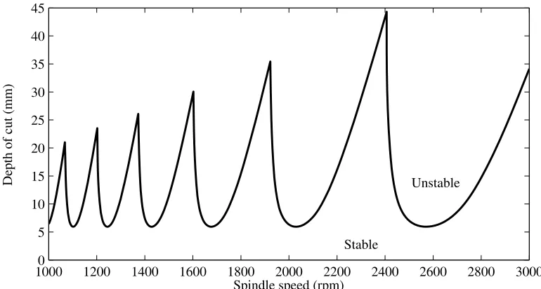
been to optimise the cutting conditions by determining the so-called stability lobe diagram [3,
4]. With reference to the example in Figure 1, it can be seen that the regenerative chatter
stability is a function of depth of cut and spindle speed. Stable cutting can be achieved by
increasing the spindle speed which has the additional benefit of increasing the material
removal rate (i.e. productivity).
An alternative approach is to increase the damping of the machine, tool, or workpiece, so as
to increase the depth of cut at which chatter occurs. Increasing the damping can be achieved
by passive [5, 6], semi-active [7-9] or fully active [10-12] means. Another seemingly elegant
method is to attempt to break up the mechanism of regenerative chatter by rapidly varying the
spindle speed [13, 14]. In practice, however, this requires very high torque from the machine
in order to overcome the inertia of the drive system.
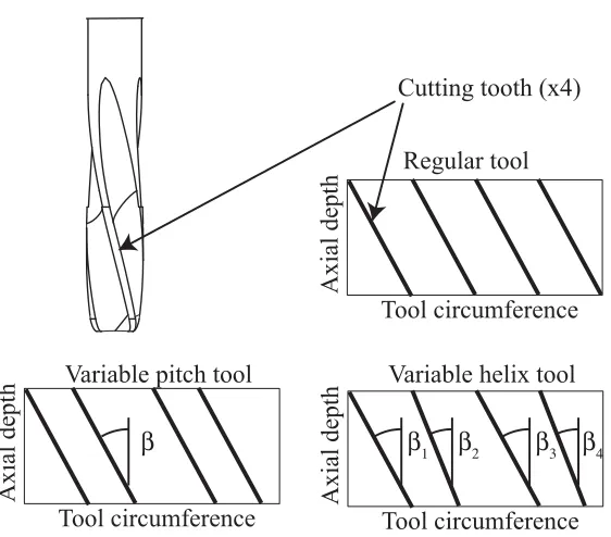
For milling problems, the regenerative affect can also be disrupted by changing the pitch
and/or helix angle of the tool flutes, as illustrated in Figure 2. For variable pitch tools at high
radial immersion, an analytical solution was developed by Altintas
et al
[15]. More recently,
this has enabled the optimisation of tool geometry [16]. A novel mathematical approach has
also been developed [17] which is well suited to the optimal design of variable pitch tools.
In recent years, the behaviour of milling tools at low radial immersions has been studied in
detail. In this configuration, the milling tool is often not engaged in the workpiece. This
by a period doubling or flip bifurcation as opposed to the usual secondary Hopf bifurcation.
The stability of interrupted cutting has been studied by Merdol and Altintas [18] (who used a
Fourier series expansion of the periodic cutting forces), Insperger
et al
[19, 20] ( who used a
semi-discretisation approach) and Mann
et al
[21] who used a temporal finite element
method). It should be noted that to the authors’ knowledge none of this previous work has
demonstrated the existence of cyclic fold bifurcations, and it has focussed on regular pitch
and regular helix tools.
Furthermore, to the authors’ knowledge there has been very little work to predict the stability
of variable helix tools in either high or low radial immersions. One exception is the work by
Turner
et al
[22]. They proposed that variable helix tools could be modelled by taking the
average pitch for each flute, and then applying the variable pitch stability analysis from
reference [15]. They showed that the results were acceptable when the axial engagement of
the tool was low so that the variable pitch approximation remained valid. They also proposed
that differences between experimental results and time-domain simulation results could be
attributed to the process damping phenomenon.
The present contribution proposes three model formulations that will be referred to as
semi-analytical formulations. The first is a semi-discretisation method, motivated by [19, 20] but
suitable for variable pitch/helix tools. The second is a time-averaged semi-discretisation
simplification that has similar assumptions to reference [15]. The third is a temporal finite
element method based upon reference [23], that is capable of modelling variable pitch tools at
low radial immersions with a uniform constant helix angle. Compared to earlier work, the
novel contribution of these methods is that they can predict the stability of:
Variable pitch tools at low radial immersion
Variable helix tools at low radial immersion
Variable helix tools at high radial immersion
pitch scenario is then presented, and the results compared to time-domain simulations.
Finally, variable helix scenarios are presented for low and high radial immersions, and
compared to time-domain simulations.
2
Regenerative chatter
Before presenting the theoretical basis for the proposed modelling methods, it is worthwhile
to briefly summarise the mechanism of regenerative chatter, for the sake of completeness.
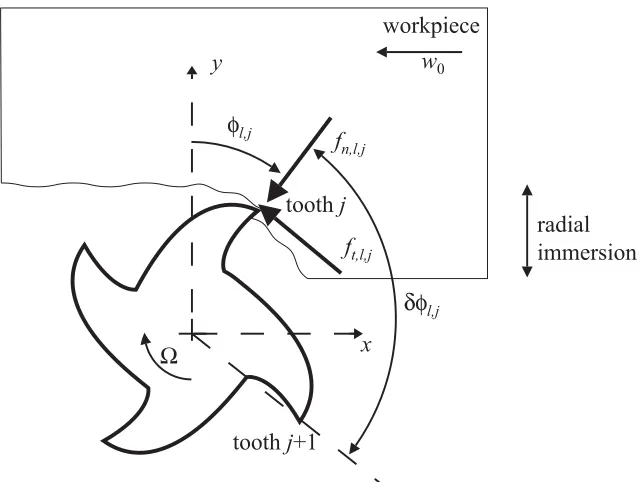
Consider a milling tool (such as that shown in Figure 2), that is up-milling a workpiece. The
forces and displacements on a plane normal to tool axis are shown schematically in Figure 3.
The forces acting on each tooth can be considered to be a function of the thickness of the chip
being removed by that tooth. These forces will cause a relative motion between the tool and
the workpiece in the
x
and
y
directions. This relative motion imparts a wavy surface finish on
the just-cut workpiece, and as the tool rotates this wavy surface is cut by the next tooth. The
chip thickness is therefore a function of the current relative displacement and that when the
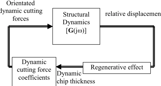
previous tool was cutting the workpiece at this location. The result is a natural feedback
process, or self-excited vibration, that can be represented by the schematic block diagram in
Figure 4.
In the following sections, models will be developed in order to predict the stability of this
self-excited behaviour for variable pitch and/or helix milling tools.
3
Semi-discretisation method
In this method, the semi-discretisation method [19, 20] is adopted, but reformulated with a
state-space approach to enable its use on variable pitch and variable helix tools. The
methodology can be separated into three aspects: discretisation, cutting force modelling, and
state-space formulation. These aspects will now be described.
3.1
Discretisation
Returning to Figure 2, it can be seen that for variable helix tools the delay between each flute
varies along the axial depth of the tool. This can be tackled by discretising the tool into
L
axial layers with depth
b
=
b
/
L
, and discretising in the time domain so that
N
time steps occur
in one tool revolution. For consistency with the literature on discrete-time systems [24], the
contrast to regular pitch tools that are usually considered periodic with each tooth-pass. The
integer variable
n=
1,2,…,
N
will be used to define the discrete local time
nT
within each tool
revolution.
The relationship between spindle speed
(rad/s) and sampling time period
T
is therefore:
N
T
2
(1)
As the tool rotates through one complete revolution, the angular position of each axial layer of
each flute varies periodically as follows:
n
N
N
n
T
nT
l jj
l
1
,
2
,...,
2
0
,
,
(2)
where
l,j(0T) defines the flute geometry of the tool as an angle (in units of radians) from the
tool axis to the flute’s cutting edge, for each axial discretisation layer
l
and each flute
j
.
The pitch between one tooth and the next is given by:
tt t
j l l
j l j
l j
l
j
N
N
j
N
j
T
T
T
T
,...,
1
2
0
0
0
0
, 1
,
, 1
,
,
(3)
where
N
tis the number of teeth on the tool. The corresponding time delay between one flute
and the next can be described by integer multiples of the sample time
T
:
2
round
,,
j l j
l
T
N
(4)
where the function
round
represents the rounding of a real number to the nearest integer.
An example is shown in Figure 5. Here, the 16mm diameter tool has two teeth that are 150°
and 210° apart at the tool tip. The teeth have helix angles of 50° and 40°. A sample time
T
is
chosen that is
N
=60 times greater than the spindle speed, so that the tool circumference (0 to
360°) can be represented in delay coordinates (0, 1, …, 60). The fluted region of the tool is
divided into five equally sized axial layers of depth
b
=0.002m. For each slice
l
of the tool,
the delay between one tooth and the next can be obtained by rounding the physical flute
position
l,j(0T) into an integer delay coordinate. For this example the time delays
are
LNtT
21
39
22
38
23
37
24
36
25
35
(5)
3.2
Cutting force modelling
A discretised axial layer of the milling cutter that is engaged in the workpiece is considered in
Figure 3. Assuming a circular tool path and a feed per tooth
w
0, the chip thickness for tooth
j
on layer
l
is given by [25-27]:
n
N
k
nT
kT
u
kT
u
nT
kT
u
kT
u
nT
w
nT
g
w
j l j l y y j l j l x x j l j l j l,...,
2
,
1
,...
2
,
1
cos
sin
sin
, , , , , 0 , ,
(6)
where
u
xand u
yare the relative vibrations between the tool and workpiece in the
x
and
y
directions respectively. The function
g
is a unit step function which has value unity when
flute
j
at layer
l
is engaged in the workpiece:
or
0
1
, , , , ex j l j l st ex j l st j lnT
nT
nT
nT
g
(7)
Here,
stand
exdefine the angles at which the teeth enter and leave the workpiece. As with
previous literature [25] the static component
w
0sin(
l,j) in (6) is neglected in the stability
analysis because it does not contribute to the regenerative effect. Clearly, the chip generation
process depends upon the difference between current relative displacements
u
x,
u
y, and
displacements at previous time points. Unlike uniform pitch tools, however, the time delay
is not constant for each tooth or axial layer. Consequently, it is useful to define an
intermediate state variable
that describes the difference between the current discrete-time
displacements and the
N
previous discrete-time displacements within the last revolution:
kT
u
kT
u
kT
nT
nT
kT
u
kT
u
kT
y y n y x x n x
(8)
The vector
x y
Thas size [2Nx1], and each element describes the vibration relative
Returning to Figure 3, it is commonly assumed [23, 25] that the forces acting on each flute are
proportional to the chip thickness, giving:
j l t r j l n j l t j l t
f
K
f
w
b
K
f
, , , , , , ,
(9)
which leads to corresponding forces in the
x
and
y
directions:
l j nl j
l j j l t j l y j l j l n j l j l t j l xf
f
f
f
f
f
, , , , , , , , , , , , , , , ,cos
sin
sin
cos
(10)
Substituting (6) and (9) into (10) gives:
yx x x l j yy y y l j
t j l y j l y y xy j l x x xx t j l x
kT
u
kT
u
a
kT
u
kT
u
a
bK
f
kT
u
kT
u
a
kT
u
kT
u
a
bK
f
, , , , , , , ,
(11)
where the instantaneous time varying directional coefficients are:
lj
l j r
l j
yy j l r j l j l yx j l r j l j l xy j l r j l j l xx
K
g
a
K
g
a
K
g
a
K
g
a
, , , , , , , , , , , ,2
cos
1
2
sin
2
sin
2
cos
1
2
sin
2
cos
1
2
cos
1
2
sin
(12)
The averaged directional coefficients
within
each discretisation time step
T
can be obtained by
integration. In general:
N Nad
N
g
a
2
(13)
where the limits of the integration are chosen so that they span an angle 2
/N, which is the
angle by which the tool rotates for each discrete-time step. This gives:
nT NN nT r r j l yy N nT N nT r j l yx N nT N nT r j l xy N nT N nT r r j l xx j l j l j l j l j l j l j l j l
K
K
N
g
a
K
N
g
a
K
N
g
a
K
K
N
g
a
, , , , , , , ,2
sin
2
2
cos
4
2
cos
2
2
sin
4
2
cos
2
2
sin
4
2
sin
2
2
cos
4
, , , ,(14)
Note that these direction coefficients vary periodically with each revolution of the tool. The
t
yx
x
x
l j
yy
y
y
l j
j l y j l y y xy j l x x xx t j l xkT
u
kT
u
a
kT
u
kT
u
a
bK
kT
f
kT
u
kT
u
a
kT
u
kT
u
a
bK
kT
f
, , , , , , , ,
(15)
These forces can be summed for all teeth and all axial discretisation layers to give the
resultant forces,
F
xand
F
y, in the
x
and
y
directions. A corresponding matrix formulation can
then be developed by using the variable
introduced in (8):
kT
kT
nT
kT
F
kT
F
y x y xR
(16)
The elements of the periodic time-varying matrix
R
are populated as follows:
t t t t N j L l j l yy j l t k N N j L l j l yx j l t k N N j L l j l xy j l t k N j L l j l xx j l t knT
a
k
h
bK
nT
r
nT
a
k
h
bK
nT
r
nT
a
k
h
bK
nT
r
nT
a
k
h
bK
nT
r
1 1 , , , 2 1 1 , , , 1 1 1 , , , 2 1 1 , , , 1,
2
1
,
2
1
,
2
1
,
2
1
(17)
where
h
is a unit step function that defines the appropriate delay term:
T
k
T
k
k
h
j l j l j l , , ,0
1
,
(18)
3.3
State-space formulation
Returning to Figure 3, the relative motion between the tool and workpiece in the
x
and
y
directions have been defined as
u
xand
u
y, respectively. In the present work these are assumed
to be the same for all axial layers of the tool. This relative motion arises due to the structural
dynamics of the tool or workpiece, which can be represented in state-space form as:
s s s s s sx
C
B
x
A
x
1 2 1 y x y x Du
u
F
F
(19)
where the subscript s denotes the structural dynamics, and
D
is the total number of states used
Discretising the continuous time dynamics (19) gives:
kT
kT
u
kT
u
kT
F
kT
F
kT
T
kT
m y x y x m m mx
C
B
x
A
x
s m
(20)
where
A
mand
B
mare given by the matrix exponential:
2 2 2 2 2 2 2exp
0
0
B
A
B
A
s sm m D D D D D D D D
D
T
(21)
Meanwhile, the relationship between the relative vibration
u
and the delay state
can be
represented in discrete-time state-space form as:
kT
u
kT
u
kT
kT
kT
kT
u
kT
u
kT
T
kT
y x y x y x d d d d d d dD
x
C
B
x
A
x
(22)
The terms in (22) are:
T N T N T N T N N N N N T N T N T N T N N T N N N N T N N NI
I
1
1
0
0
0
0
1
1
0
0
0
0
1
0
0
0
0
0
0
1
0
0
0
0
0
0
0
0
0
0
0
0
1 1 1 1 1 1 1 1 1 1 1
d d d dD
I
I
C
B
A
(23)
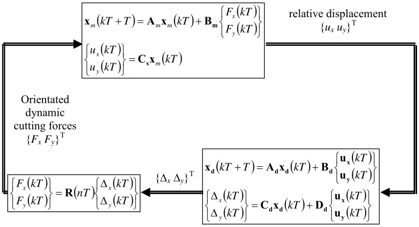
The schematic block diagram shown in Figure 4 can now be replaced by the mathematical
model shown in Figure 6. Combining (20), (22) and (16) gives:
d s
s
m d s d
m
C
R
C
D
R
C
0
B
B
A
C
B
0
A
A
nT
nT
nT
N
2 2
(25)
Consequently the states of the system vary between one tool revolution and the next tool
revolution as follows:
kT
kT
T
T
N
NT
NT
kT
NT
kT
d m
d m
x
x
BC
A
BC
A
BC
A
x
x
1
(26)
The asymptotic stability of the system is therefore governed by the eigenvalues or
characteristic multipliers of
A
BC
NT
A
BC
N
1
T
A
BC
T
. Characteristic
multipliers (CM’s) with magnitude greater than unity indicate an asymptotically unstable
system, i.e. chatter, and the value of the maximum CM as it crosses the unit circle indicates
the type of bifurcation which occurs [28]. For a secondary Hopf or Neimark bifurcation, the
maximum CM crosses the unit circle with a non-zero imaginary component, and
quasi-periodic motion occurs. For a period doubling or flip bifurcation, the maximum CM crosses
the unit circle at -1, and period two motion occurs. For a saddle-node or cyclic fold
bifurcation, the maximum CM crosses the unit circle at +1, and period one motion occurs.
Cyclic fold bifurcations are often associated with the ‘jump phenomenon’ where the periodic
motion is replaced by another remote solution as the control parameter (i.e. depth of cut) is
increased [28]. To the authors’ knowledge, cyclic fold bifurcations have not been observed in
previous work on milling chatter, except where it arises due to tool runout [29]. However, it
should be noted that Insperger and Stepan [30] identified similar behaviour during turning
operations with a periodically varying spindle speed.
4
Time averaged semi-discretisation approach
In this section, the semi-discretisation method will now be simplified slightly. A considerable
amount
of
computation
time
is
required
to
compute
the
product
A
BC
NT
A
BC
N
1
T
A
BC
T
in Eq. (26) when the order
N
is large. This
issue can be avoided if the time varying direction coefficients are averaged across an entire
ex stad
N
ad
N
g
2
2
2 0(27)
This is equivalent to the assumption used by Budak and Altintas [31] who expressed the
direction coefficients as a Fourier series and selected only the first term in the series. The
resulting time-averaged direction coefficients are:
exst ex st ex st ex st r r yy r yx r xy r r xx
K
K
K
K
K
K
2
sin
2
2
cos
4
1
2
cos
2
2
sin
4
1
2
cos
2
2
sin
4
1
2
sin
2
2
cos
4
1
(28)
It should be noted that these differ from the values given by Altintas [25] by a factor of
N
t,
because in the present formulation the summation for all teeth occurs separately. Since these
coefficients are no longer periodically time varying, Eq. (16) can be rewritten with a constant
value for
R
:
kT
kT
kT
F
kT
F
y x y xR
(29)
Where the constant elements of
R
are:
t t t t N j L l yy j l t k N N j L l yx j l t k N N j L l xy j l t k N j L l xx j l t kk
h
bK
r
k
h
bK
r
k
h
bK
r
k
h
bK
r
1 1 , , 2 1 1 , , 1 1 1 , , 2 1 1 , , 1,
2
1
,
2
1
,
2
1
,
2
1
(30)
The state-space representation of the system is now given by:
n
N
d s s
m d s d
m
C
C
RD
C
0
B
B
A
C
B
0
A
A
2 2N
(32)
Consequently, stability can be determined directly from the eigenvalues of (
A
+
BC
).
The advantages of this time-averaged semi-discretisation formulation are twofold. First, the
computation time is faster as previously mentioned. Second, the formulation is equivalent to
the method of Altintas and Budak [31] in that the direction coefficients are time-averaged in
the same fashion. This allows the axial and temporal discretisation methodology to be
validated by a direct comparison with published work on variable pitch tools.
5
Time Finite Element Formulation
A key issue with the previous two methods is that they perform axial discretisation of the tool,
as well as discretisation in the time domain. Although the convergence of time domain
semi-discretisation was investigated by reference [19], axial semi-discretisation has not previously been
considered for semi-analytical models. It is therefore important to compare the stability
predictions with those from alternative models that do not perform axial discretisation of the
tool. Recent work by Patel, Mann, and Young [23] has investigated the stability of uniform
pitch tools at low radial immersions, and shown that the constant helix angle of the tool has a
significant effect on the period doubling bifurcation behaviour. This method performed
analytical integration over the axial length of the tool, and the approach will now be extended
to consider the case of a variable pitch tool, under the assumption that only one flute is
engaged in the workpiece at any one point in time. For the sake of brevity, a full derivation is
not presented here. Instead, the theory described by [23] is briefly outlined, with emphasis on
modification of the approach for the case of variable pitch tools. It should be noted that this
will enable the constant helix angle of a variable pitch tool to be considered, but the approach
is not yet suitable for variable helix angle tools.
Patel
et al
[23] considered a single-degree of freedom vibration aligned with the tool feed
direction (i.e. the
x
-direction of Figure 3). They showed that the cutting force in the
x
K
K
K
dz
t
u
t
u
w
t
z
g
F
t t rt z
t z
x x
x
2
cos
1
2
sin
2
,
2
1
0
(33)
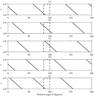
The limits of integration were shown to be piecewise continuous and can be summarised
graphically with the help of Figure 7. In the first regime (Figure 7a) a flute is entering the cut,
whilst in the second regime (Figure 7b) a flute is in the middle of the cut (and may or may not
be engaged in the workpiece across its entire length). In the third regime (Figure 7c) the tool
leaves the cut, and this is followed by a period of time where there are no cutting forces and
the tool experiences a free vibrational decay (Figure 7d). This process is then repeated for the
next flute on the tool (Figure 7e).
For a uniform pitch tool, the solution to the equation of motion is periodic for each flute
(Figure 7a to d). Whilst an analytical solution for the free decay behaviour (Figure 7d) is
straightforward, the behaviour during cutting is described by a delay-differential equation
which is solved with an approximation method. Patel [23] and previous authors [29] have
applied the temporal finite element analysis (TFEA) method, which allows the
delay-differential equation to be transformed into a discrete map.
To implement the TFEA method, the delay-differential equation is first written in state-space
form as:
t
A
t
t
y
t
B
t
t
y
t
y
(34)
Where
A
tis the state matrix and
B
tis the delayed state matrix. An assumed solution is used
for the states
y
and the delayed states
y
(
t-
). The method of weighted residuals is then applied
to the assumed solution, so as to minimise its error [32]. The results from each temporal
element can then be combined, along with the equation describing the free-decay behaviour,
to form a discrete map in the form:
,...
2
,
1
1
jj
j
Qy
y
(35)
which describes the states of the system for each tooth pass
j
as a function of the states for the
previous tooth pass
j
-1.
It transpires that this procedure can be readily extended to the problem of variable pitch tools
provided that only one tool is in contact with the workpiece at any one point in time. The
method of Patel
et al
[23] is simply applied to each flute of the tool in turn. The matrix
Q
will
Consequently, Eq. (34) and (35) must be rewritten for each flute, leading to the behaviour
from one
tool revolution
to the next:
t t
t N j N
N
j
Q
Q
Q
y
y
1
1(36)
The stability of the system can therefore be determined by the eigenvalues or characteristic
multipliers of the product
Q
Q
1
Q
1t
t N
N
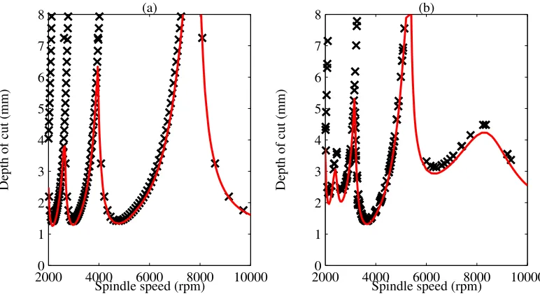
![Figure 9: Stability lobes for the single-degree of freedom flexure considered by Patel and Mann [23]](https://thumb-us.123doks.com/thumbv2/123dok_us/8078640.228427/37.612.105.487.70.516/figure-stability-single-degree-freedom-flexure-considered-patel.webp)
