Ameliorating the FOPID (PIλDμ) controller parameters for heating furnace using optimization techniques

Abstract

Since the heating furnace system has emanated it has faced the problem of high power consumption, colossal amount of time to heat the substances and the vulnerability of getting exploded thus the objective of the paper is to achieve a system for same with less power consumption, whit time to heat the substances and making it safe from explosion.

Using the mathematical way of modeling the dynamic critical systems the heating furnace is being modeled by using the damping, spring and mass elements. The integer order model of the system is being achieved by the Laplace transform and fractional order model for the same is obtained using the Grunwald-Letnikov formula. The Cohen-Coon tuning technique is being amalgamated with the Nelder-Mead, Interior-Point, Active-Set and Sequential Quadratic Programming optimization techniques respectively so as to design the FOPID controller for heating furnace.

When the feedback systems were being formed then the outputs demonstrated that the system now consists the properties of less power consumption, less time to heat the substances along with less overshoot. Earlier the integer order model had the settling time (time taken to heat the substance), steady state error (power consumption) and overshoot (explosion) of 1500 seconds, 50% and 0% respectively. When the PID controller was designed for the same using Cohen-Coon tuning technique and forming a feedback system it had setting time of around 800 sec. and also the steady state error was brought to 0% but the overshoot went up to 35%. Therefore FOPID controller is being designed using the concocted technique that is the amalgamation of tuning technique and optimization techniques and forming and feedback system with FOM of heating furnace, the system yielded steady state error as 0%, where the settling time have been reduced to 300 seconds and overshoot between 7%-12%.

Using the concocted technique that is the amalgamation of Cohen-Coon tuning technique with the optimization tuning techniques the FOPID controller was being formed for the FOM of the heating furnace which is being kept in feedback so as to form a system. Thus systems formed ameliorated the settling time i.e. time taken to heat the substance, the overshoot i.e. the vulnerability of getting exploded also remains low and the steady state error i.e. power consumption is also reduced drastically.

Ameliorating the FOPID (PIλDμ) Controller

Parameters for Heating Furnace using

Optimization Techniques

Amlan Basu

_{, Sumit Mohanty and Rohit Sharma}

Department of Electronics and Communication Engineering, ITM University, Gwalior - 474001, Madhya Pradesh, India; [email protected], [email protected], [email protected]

Keywords: FOPID Controller, Heating Furnace, Optimization Techniques, Overshoot, Settling Time, Steady State Error

1. Introduction

It is fascinating to note that almost 90% of the modern controllers being used today are the Proportional Integral Derivative (PID) controller or the modified Proportional Integral Derivative (PID) controller.

Proportion Integral Derivative (PID) controller is the controller which is of the integer order and it is being

utilized widely in the field of industry. The controller appeared in the year 1939 and from that point forward it has stayed crucial in view of its execution. Since most of the Proportional Integral Derivative (PID) controllers are balanced nearby, a wide range of sorts of tuning principles have been proposed in the literature. Utilizing the tuning standards, sensitive and calibrating of Proportion Integral Derivative (PID) controllers can be made on site. Likewise,

*Author for correspondence

programmed tuning techniques have been created and a percentage of the Proportional Integral Derivative (PID) controller may have online programmed tuning capacities. Adjusted types of Proportion Integral Derivative (PID) control, for example, I-PD control and multi degrees of freedom Proportion Integral Derivative (PID) control are right now being used in industry. Numerous pragmatic systems for bump less changing (from manual opera-tion to programmed operaopera-tion) and increase booking are economically accessible. The handiness of Proportion Integral Derivative (PID) controls lie in their general per-tinence to most control frameworks. Specifically, when the scientific model of the plant is not known and in this way investigative outlines strategies can’t be utilized, Proportional Integral Derivative (PID) controls ends up being generally helpful. In the field of procedure control frameworks, it is surely understood that the fundamental and the modified Proportional Integral Derivative (PID) control strategies have demonstrated their helpfulness in giving palatable control, in spite of the fact that in numer-ous given circumstances they may not give ideal control. Mathematically the Proportional Integral Derivative (PID) controller using differential equation is1,23_,

(1) Where,

K_p designates the gain of Proportional, K_i designates

the gain of Integral, Kd designates the gain of Derivative, e

designates the Error, t designates the Instantaneous time and τ designates the variable of integration that takes on the values from time 0 to the present t.

The transfer function of Equation (1) is2,23_,

(2)

Here, we are using the FOPID controller which has been derived from the Proportional Integral Derivative (PID) controller by just converting it into fractional order from the integer order which was first being proposed in 1999 by Igor Podlubny. In addition, the incentive behind the utilization of FOPID is that it is very easy to design the controller for systems with higher order by using the tech-niques of modeling based on regression and also because it has the iso-damping property which makes possible the variation over wide range of operating point for a singular controller. There are numerous other grounds which are liable for the utilization of FOPID controller and they are the heftiness from the high frequency noise as well as for

the gain variation of the plant, the absence of the steady state error and it contains both the phase and gain margin and also the gain and phase cross over frequency.

The FOPID controller can further be defined numerically using differential Equation as,

(3) And the transfer function of the Equation (3) is given as,

(4)

{λ, μ} in Equation (4) designates the Differential-integral’s order for FOPID controller3_.

Optimization also termed as enhancement is the system of making the things more flawless, powerful and productive in order to yield the best result. The various techniques of optimization are Nelder-Mead, Active-Set, Interior-Point, SQP (Sequential Quadratic Programming) etc23_{. Numerically it can be explained as the system of} expansion and contraction of the target capacity relying upon various decision variables under an arrangement of limitations. The optimization technique has been used so as to find and achieve the finest results so as to design the most accurate FOPID controller that gives the finest

output and assists the plant to enhance its performance4_.

Since the classical calculus cannot solve the equations with fractional order therefore the fractional calculus has been used extensively here. Basically the fractional calculus is numerical computation that scrutinizes the likelihood of accepting the real and complex number powers of operator of differentiation.

2. Modeling of Heating Furnace

Dynamically

The modeling that has been approximated for the heating furnace rivets amount of input that varies with time and is in fact the fuel mass gas flow rate and also the pressure inside the furnace which is the output value.

The modeling of heating furnace dynamically rivets

the mass, energy and the momentum balances23_{. It also}

rivets the heat transfer from the hot flue hot gas to water,

flue gas flow from the boiler model and steam model5_.

As we know for any physical system the total force is equal to the summation of individual forces exerted by

mass (m), damping (b) and spring (k) element23_.

(5)

In the Equation (4) acceleration is signified as a, velocity is signified as v and displacement is signified as x23_.

Therefore the differential equation of Equation (4) is,

(6)

It must be accounted that for designing a network based PID the above equation or model is a rough process behavior description6,23_.

Therefore, the differential equation of the heating

furnace using the above equation becomes23_,

(7)

The Laplace transfer function of Equation (6) which

gives the Integer Order Model (IOM) as23_,

GI(s) = (8)

‘s’ in Equation (8) signifies the Laplace operator7,23_. Where, the mass denoted by ‘m’ is 73043, the damping denoted by ‘d’ is 4893 and the spring denoted by ‘k’ is 1.93 23_.

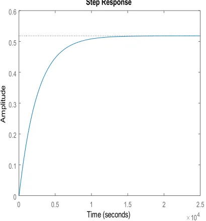
From Figure 1 it can be very well said that when the heating furnace is being modeled in integer order then

overshoot is 0%, the steady state error is around 50% and the settling time is 1500 seconds.

3. A Precis on Fractional Order

Calculus

Fractional order calculus is a mathematical concept that has been in existence from 300 years ago. It is the mathematical concept that has proved itself better as compared to the integer order methods.

The definition of the fractional order calculus is as follows:

According to Lacroix8_,

(9)

According to Liouville9_,

( )

(

)

( ) ( )

( )

1

1 _{2 1} 1

2 2 2

1 2

1 1 2

u x u a d f

D f x u f u du F x

l d x a

−

− _{= −} −

− ₌

= − =

 

−  _{ }

∫

(10)

According to Riemann-Liouville10_,

(11)

According to Grunwald-Letnikov, which is being used widely is,

(12)

Where,

(13)

Which is called the Euler’s gamma function11_.

The fractional order derivatives and integrals properties are as follows:

f (t) being a logical function of t then the fractional •

derivative of f (t) which is ₀ is an analytical

function of z and α.

If α = n (n is any integer) then

• ₀ produces the

similar result as that of the traditional differentiation having order of n.

If α = 0 then

• ₀ is an identity operator.

0 0.5 1 1.5 2 2.5

104

0 0.1 0.2 0.3 0.4 0.5

0.6 Step Response

Time (seconds)

A

m

p

lit

u

d

e

0 (14)

The differentiation and integration of fractional order •

are said to be linear operations10_,

0 (15)

The semi group property or the additive index law, •

0 0 =0 0 =0 (16)

Which is being held under some sensible limitations on f (t).

Derivatives which are of fractional order has the commutation with derivative of integer order which is as follows12_,

a a a (17)

Where for t = a, f (k) _{(a) = 0 for k = {0, 1,…n-1}. The given}

equation shows that and _a are commuted 13_.

4. Cohen-Coon Tuning Technique

Cohen-Coon tuning technique is primarily used to vanquish the slow, steady state response which takes

place in the Ziegler-Nichols tuning technique11_{. This}

tech-nique is generally utilized for the systems with first order or models having time delay as the controller does not spontaneously responds to the disturbances.

It is an offline method that is when it is at steady state then a step change can be introduced at the input. After this on the basis of the time constant and the time delay the output can be calculated and the initial control

parameters can be found out using the response11_.

To get minimum offset and standard decay ratio there are an arrangement of pre-decided settings for the Cohen-Coon tuning technique,

Where, P is the percentage in the input, N is percentage

change of output/ τ, L is τ_dead and R is . We

can use Ko in place of .

The procedure of the tuning technique is as follows:

Wait for the complete procedure till the steady state is •

attained.

Step change is to be introduced at the input. •

Approximate first order constant with time constant •

τwhich is delayed by τ_dead units which is based on the

output, from the time the step input was introduced. By recording the following time instances the value of τ and τ_dead can be found, t₀ signifies the input step start up point, t₂ signifies the half point time and t₃ signifies the time at 63.2%.

Calculate the process parameters τ, τ

• dead and Ko by

utilizing the assessment done at t₀, t₂, t₃, A and B. On the basis of τ, τ

• _dead and K₀ the parameters of

controller can be found.

The advantages of the Cohen – Coon method are that the time of reaction of the closed loop is quick or fast and this technique can be utilized in the systems along with time delay.

Whereas the disadvantages of this technique are that it can only be utilized for the first order systems which involve large process delay, it is an offline technique, closed loop systems are unstable and the approximated value of τ, τdead and K0 might not be compulsorily accurate

for different systems14_.

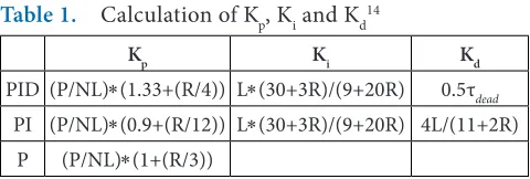
From Table 1 it can be derived that using various

formulae the tuning parameters i.e. proportional gain K_p,

integral gain Ki and derivative gain Kd can be obtained

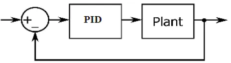
spe-cifically when the Cohen-Coon technique is being used. When the Equation (8) which is the Integer Order Model (IOM) of the heating furnace is placed in a closed loop along with the PID controller which is tuned using the Cohen-Coon tuning technique as shown in the Figure 2 then the step response that we get is shown in Figure 3.

From Figure 3 it can be said that the settling time drastically reduced and also the steady state error also reduced to 0% but at the same time the overshoot increased a lot which is certainly not acceptable and all these happened when the PID controller was used.

5. Nelder-Mead Optimization

Technique

Nelder-Mead optimization technique is also called the Downhill simplex technique or the amoeba technique

Table 1. Calculation of Kp, Ki and Kd14

Kp Ki Kd

PID (P/NL)∗(1.33+(R/4)) L∗(30+3R)/(9+20R) 0.5τ_dead PI (P/NL)∗(0.9+(R/12)) L∗(30+3R)/(9+20R) 4L/(11+2R)

which is used to find the minimum and maximum of an objective function in various dimensional spaces23_{. The} Nelder–Mead method is a technique which is a heuris-tic search method that can coincide to non-stationary points. However, it is easy to use and will coincide for a

large class of problems23_{. The Nelder–Mead optimization}

method was proposed by John Nelder and Roger Mead in year 1965. The procedure uses the concept of a simplex (postulation of notion of triangle or tetrahedron to arbi-trary dimensions) which is a special polytope (geometric objects having flat sides) type with N + 1 vertices at n

dimensions23_{. Illustrations of simplices are, a tetrahedron}

in three-dimensional space, a triangle on a plane, a line segment on a line, etc.

The different operations in Nelder-Mead optimization method are23_,

Taking a function f (x), x ∈ Rn _{which is to be minimized}

in which the current points are x₁, x₂ ……. x_n+123_.

Order: On the basis of values at the vertices, f (x

• 1) ≤ f

(x₂) ≤ …………. ≤ f (x_n+1)23_.

Calculate the centroid of all points (x

• ₀) except x_n+123_.

Reflection: Calculate x

• _r = x₀+ α (x₀ – x_n+1)23_{. If the}

reflected point is not better than the best and is better than the second worst, that is, f (x₁) ≤ f (x_r) < f (x_n)23_. After this by replacing the worst point x_n+1 with

reflected point x_r to get a new simplex and go to the

first step23_.

Expansion: If we have the best reflected part then f •

(x_r) < f (x₁), then solve the expanded point x_e= x₀+γ (x₀-x_n+1)23_{. If the reflected point is not better than} expanded point, that is, [f (xe)<f (xr)] then either by

substituting the worst point x_n+1 by expanded point x_e

to get new simplex and then go to the first step or by replacing the worst point x_n+1 by reflected point x_r to obtain or get a new simplex and then go back to the first step23_.

Else if the reflected point is not better than second •

worst then move to the fifth step23_. Contraction: Here we know that f (x

• r) ≥ f (xn)23,

contracted point is to be evaluated x_c= x₀+ρ (x₀-x_n+1), if f (x_c) < f (x_n+1) that is the contracted point is better than the worst point then by substituting the worst point

xn+1 with contracted point xc to procure a new simplex

and then go to first step or proceed to sixth step23_. Reduction: Substitute the point with x

• _i= x₁+σ (x_i-x₁)

for all i ∈ {2, ……. ,n+1}23_{, then go to the first step.}

It must be noted that the standard values for α, σ, ρ, γ are 1, ½, -1/2, 2 respectively. In reflection the highest

valued vertex is xn+1 at the reflection of which a lower

value can be found in the opposite face which is formed by all vertices x_i except x_i+1. In expansion we can find

fascinating values along the direction from x₀ to x_r only

if the xr which is the reflection point is new nadir along

vertices. In contraction it can be expected that a superior value will be inside the simplex which is being formed by the vertices x_i only if f (x_r) > f (x_n). In reduction to find a simpler landscape we contract towards the lowest point when the case of contracting away from the largest point increases f arises and which for a minimum non-singular cannot happen properly. Indeed initial simplex is important as the Nelder-Mead can get easily stuck as too small inceptive simplex can escort to local search,

Figure 2. Closed loop with PID controller and the heating furnace (plant).

0 100 200 300 400 500 600 700 800 900 1000 Time [sec]

0 0.2 0.4 0.6 0.8 1 1.2 1.4

A

m

p

lit

u

d

e

therefore the simplex should be dependent on the type

or nature of problem15_.

6. Active-Set Optimization

Technique

In constrained optimization, the general point is to change the issue into a less demanding sub-problem that can then be understood and utilized as the prem-ise of an iterative procedure. A normal for a huge class of right on time routines is the interpretation of the compelled issue to an essential unconstrained issue by utilizing a penalty function for limitations that are close or past the imperative limit. Along these lines the compelled issue is settled utilizing a grouping of parameterized unconstrained advancements, which in the (arrangement’s utmost) focalize to the constrained problem. These routines are currently considered mod-erately wasteful and have been supplanted by systems that have concentrated on the arrangement of the Karush-Kuhn-Tucker (KKT) mathematical statements. The KKT comparisons are important conditions for optimality for a constrained improvement problem. On the off chance that the issue or problem is a purported

raised programming issue, that is, and , i =

1,….,m, are convex function, then the KKT mathemati-cal statements are both important and adequate for a global solution point23_.

Taking a general problem23_,

(18)

Therefore, the KKT equation can be given as23_,

(19)

(20)

(21) The Equation (19) depicts a crossing out of the gradient between the active constraints and the objective function

at the point of solution23_{. For the gradients to be wiped}

out, Lagrange multipliers are

impor-tant to balance the deviations in objective function’s and

constraint gradient’s magnitude23_{. Since only active}

con-straints are incorporated into this crossing out operation, inactive constraints must not be incorporated into this

operation, as the given Lagrange multipliers equivalent to 0. This is expressed verifiably in the Equations (20) and

(21) which are the KKT equations23_.

The solution of the KKT mathematical statements shapes the premise to non-linear programming calculations. These calculations endeavor to regis-ter the Lagrange multipliers specifically. Constrained quasi-Newton procedure ensures super-linear accu-mulating so as to meet second order data in regards to the KKT Equations utilizing a quasi-Newton updat-ing method. These systems are generally alluded to as Sequential Quadratic Programming (SQP) techniques, since a quadratic programming sub-problem is solved at every major iteration (also called constrained variable metric routines, iterative quadratic programming and recursive quadratic programming). The active-set opti-mization technique or algorithm is not an algorithm of large-scale16_.

7. Interior Point Optimization

Technique

Interior point optimization technique is the method or procedure that helps to evaluate both linear and

non-lin-ear problems of convex optimization23_{. It is also termed as}

barrier technique or method23_{. The interior point way to}

deal with constrained minimization is to unravel a suc-cession of estimated minimization issues. The genuine problem is23_,

(22) The estimated problem for every μ = 0 is,

(23)

There are same numbers of slack variables s_i as there

are disparity requirements in g23_{. The s}

i are limited to be

positive to keep ln (s_i) limited23_{. As μ declines to zero, the}

minimum of f_μought to approach the minimum of f. The

included logarithmic term is termed as barrier function23_.

To solve the rough problem, the algorithm utilizes one of two principle sorts of ventures at each and every reiteration, they are, the first one is the immediate stride in (x, s)23_{. This stride endeavors to comprehend the} KKT (Karush-Kun-Tucker) mathematical statements for the rough issue by means of a direct estimation23_. This is likewise called the Newton step and the second principle is the conjugate gradient step that utilizes a

trust region23_{. Naturally the algorithm first endeavors to}

a direct or immediate step. In the event that it cannot then it endeavors the conjugate gradient step. One situ-ation where it does not take an immediate or direct step is the point at which the estimated issue is not locally

convex to the current emphasize23_{. At every reiteration}

the algorithm diminishes a legitimacy function, for example23_,

The parameter may increment with reiteration number keeping in mind the goal to constrain the arrangement towards attainability. In the event that an endeavored step does not diminish the legitimacy work, the algorithm

rejects the endeavored step and endeavors another step17_.

8. Sequential Quadratic

Programming (SQP)

Optimization Technique

SQP technique speaks to the best in class in non-linear

programming techniques23_{. For example Schittkowski has}

actualized and tested a form of that outflanks each other tested technique as far as proficiency, precision and rate of

successful elucidations over countless issues23_.

In view of the work of Biggs, Han and Powell and the technique permits us to firmly imitate Newton’s strategy for compelled improvement pretty much as is finished unconstrained optimization. At every significant empha-sis, a guess is made of the Hessian of the Langrangian function utilizing a semi Newton overhauling system23_. This is then used to create a quadratic program sub problem whose arrangement is utilized to shape the quest course for a line seek technique23_{. A review of SQP is} found in Fletcher, Gill et al., Powell and Schittkowski23_.

Taking the Equations (18), (19), (20) and (21)15_{, the}

principal initiative is the detailing of a quadratic pro-gramming sub problem in light of a quadratic estimation of the Lagrangian function23_.

(24)

We abridge the Equation (18) by assuming that bound constraints have been communicated as inequality

con-straints23_{. We achieve the quadratic programming sub}

problem by the non-linear constraints23_{. The SQP is}

implemented using three stages which are, the updating the Hessian matrix, the quadratic programming solution

and the line search and merit function18_.

9. Designing of FOPID for

the Heating Furnace using

Optimization Technique

The Integer Order Model (IOM) of heating furnace, which we already equated in section (2) and we got the Equation (8), which is23_,

G_I(s) =

Now, by using the Grunwald-Letnikov Equation (12) for fractional calculus which is given as23_,

When the Integer Order Model (IOM) is being solved using the Grunwald-Letnikov equation given above then we get the Fractional Order Model (FOM) of heating furnace which comes out to be19,23_,

G_F(s) = (25)

When the Equation (25) which is the Fractional Order Model (FOM) of the heating furnace is placed in a closed loop along with the PID controller which is tuned using the Cohen-Coon tuning technique as shown in the Figure 2 then the step response that we get is shown in Figure 4.

When PID controller for FOM of the heating furnace was designed to improve the performance of heating fur-nace then of course the settling time and steady state error improved but overshoot came out to be high, which can be deduced from Figure 4.

values came out to be 151.412, 0.803807 and 4241.46 respectively.

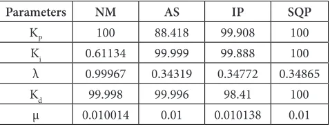
After the discussed process we use the Nelder-Mead, interior-point, active-set and SQP optimization techniques so as to find the values of λ and μ and also the optimized values of K_p, K_i and K_d which are being listed in the Table 2 given below.

Now by using the values of Table 2 and the Equation (4) we design the FOPID controller by forming its equation.

Using the values of Nelder-Mead (NM) optimization from Table 2 we get the FOPID controller Equation as,

(28)

Now, by using the values of Active-Set (AS) optimization from table we get the FOPID controller Equation as,

(29)

Now by using the values of Interior-Point (IP) optimization from Table 2 we get the FOPID controller Equation as,

(30) (26)

Where, K is referred to as the gain, L is referred as time delay and T is referred as the time constant20_.

Then, by finding out the step response of the transfer function of the plant (heating furnace) we find out the value of K, L and T.

Where, and

Where, T₁ and T₂ are the time instances in seconds

taken from the step response obtained having a particular steady state gain21_.

So, the FOPDT model for the plant which is the heating furnace comes out to be,

G_FOPDT(s) = (27)

The comparison of Equation (27) and Equation (25) is shown in the Figure 5 and form which it can be deduced that both are almost the same in performance factor.

Where the value of K, L and T we get from Equation (27) are 0.404272, 72.464 and 3421.93 respectively.

The initial values of K_p, K_i and K_d are being found out using the Cohen-Coon tuning technique whose

0 500 1000 1500

Time [sec] 0

0.2 0.4 0.6 0.8 1 1.2

A

m

p

lit

u

d

e

Figure 4. Step response obtained when the Equation (25) which is the Fractional Order Model (FOM) of the heating furnace is placed in a closed loop along with the PID controller.

Figure 5. FOPDT identification, comparison between the original and the identified one which appears to be perfect.

Table 2. Values of K_p, K_i, K_d, λ and μ found using the optimization techniques

Parameters NM AS IP SQP

K_P 100 88.418 99.908 100

Ki 0.61134 99.999 99.888 100

λ 0.99967 0.34319 0.34772 0.34865

K_d 99.998 99.996 98.41 100

(36)

10. Result

10.1 The Different Responses when

Nelder-Mead Optimization Technique

Values are used

From Figure 7 the step response achieved when the Equation (28) is put into the FOPID controller block and the Equation (25) is put into the plant block of Figure 6 and it exhibits overshoot of 12%, settling time of 1000 sec. and steady state error of 0%.

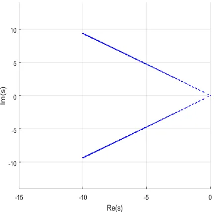
In Figure 8 the root locus obtained when the Equation (28) is put into the FOPID controller block and the Equation (25) is put into the plant block of Figure 6, this has been plotted to observe the stability of the system. Since all the zeroes lie at the second quadrant thus the system is stable.

The stability obtained when the Equation (28) is put into the FOPID controller block and the Equation (25) is put into the plant block of Figure 6, where the sys-tem came out to be stable with K = 1, q = 0.01, err =

1.1481e-10 _{and apol = 0.0281 which can be observed in}

Figure 9.

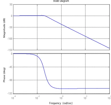
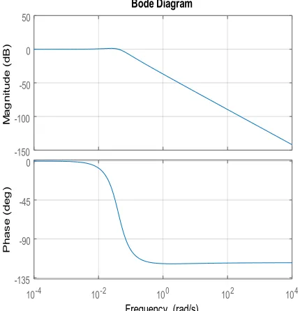
The bode plot achieved when the Equation (28) is put into the FOPID controller block and the Equation (25) is put into the plant block of Figure 6, bode plot being obtained both in phase and magnitude can be depicted from Figure 10.

Now by using the values of SQP optimization from Table 2 we get the FOPID controller Equation as,

(31)

When the Equation (28) is put into the FOPID controller block and the Equation (25) is put into the plant block of Figure 6 then the output that is obtained is22_,

(32) When the Equation (29) is put into the FOPID controller block and the Equation (25) is put into the plant block of Figure 6 then the output that is obtained is,

(34)

When the Equation (30) is put into the FOPID controller block and the Equation (25) is put into the plant block of Figure 6 then the output that is obtained is,

(35) When the Equation (31) is put into the FOPID controller block and the Equation (25) is put into the plant block of Figure 6 then the output that is obtained is,

Figure 6. Closed loop with FOPID controller and the heating furnace (plant).

0 500 1000 1500

0 0.2 0.4 0.6 0.8 1 1.2 1.4

Time [s ec]

Amplitude

10.2 The Different Responses when

Active-Set Optimization Technique Values are

used

Figure 11 shows the step response achieved when the Equation (29) is put into the FOPID controller block and the Equation (25) is put into the plant block of Figure 6, in which settling time came out to be 300 sec., overshoot of 15% and steady state error of 0%.

Figure 12 shows the root locus obtained when the Equation (29) is put into the FOPID controller block and the Equation (25) is put into the plant block of Figure 6 in which the zeroes lie in the second quadrant which allows the system to be stable.

-15 -10 -5 0

-10 -8 -6 -4 -2 0 2 4 6 8 10

Re(s)

Im(s)

Figure 8. Root locus plot for Equation (32).

-1 -0. 8 -0. 6 -0. 4 -0. 2 0 0. 2 0. 4 0. 6 0. 8 1 -1

-0. 8 -0. 6 -0. 4 -0. 2 0 0. 2 0. 4 0. 6 0. 8 1

Figure 9. Stability graph for Equation (32).

-150 -100 -50 0 50

Magnitude (dB)

10-4 10-2 100 102 104

-135 -90 -45 0

Phase (deg)

Bode Diagram

Frequency (rad/sec)

Figure 10. Bode plot for Equation (32).

0 50 100 150 200 250 300 350 400 450 500 0

0.2 0.4 0.6 0.8 1 1.2 1.4

Time [sec]

Amplitude

Figure 11. The step response of Equation (33).

-15 -10 -5 0

-10 -5 0 5 10

Re(s)

Im(s)

-1 -0.8 -0.6 -0.4 -0.2 0 0.2 0.4 0.6 0.8 1 -1

-0.8 -0.6 -0.4 -0.2 0 0.2 0.4 0.6 0.8 1

Figure 13. The stability graph of Equation (33).

-150 -100 -50 0 50

Magnitude (dB)

10-4 10-2 100 102 104

-135 -90 -45 0

Phase (deg)

Bode Diagram

Frequency (rad/s ec)

Figure 14. The bode plot for Equation (33).

0 50 100 150 200 250 300 350 400 450 500 0

0.2 0.4 0.6 0.8 1 1.2 1.4

Time [sec]

Amplitude

Figure 15. The step response for Equation (34). Figure 13 shows the stability obtained when the

Equation (29) is put into the FOPID controller block and the Equation (25) is put into the plant block of Figure 6, where the system came out to be stable with K = 1, q = 0.01, err = 838e-10 _{and apol = 0.0236.}

Figure 14 is the bode plot obtained when the Equation (29) is put into the FOPID controller block and the Equation (25) is put into the plant block of Figure 6, both in magnitude and phase.

10.3 The Different Responses when

Interior-Point Optimization Technique

Values are used

Figure 15 is the step response achieved when the Equation (30) is put into the FOPID controller block and the Equation (25) is put into the plant block of Figure 6, in which the settling time is 300 seconds, overshoot of 15% and steady state error of 0%.

Figure 16 demonstrates the step response achieved when the Equation (30) is put into the FOPID controller block and the Equation (25) is put into the plant block of Figure 6, in which all the zeroes lie in the second quadrant and from which it can be depicted that the system is stable.

Figure 17 shows the stability obtained when the Equation (30) is put into the FOPID controller block and the Equation (25) is put into the plant block of Figure 6, where the system came out to be stable with K = 1, q = 0.01,

err = 9.9290e-10 _{and apol = 0.0236.}

Figure 18 is the bode plot obtained when the Equation (30) is put into the FOPID controller block and the Equation (25) is put into the plant block of Figure 6, in both magnitude and phase.

-15 -10 -5 0

-10 -5 0 5 10

R e(s)

Im(s)

-1 -0.8 -0.6 -0.4 -0.2 0 0.2 0.4 0.6 0.8 1 -1

-0.8 -0.6 -0.4 -0.2 0 0.2 0.4 0.6 0.8 1

Figure 17. Stability plot for Equation (34).

-150 -100 -50 0 50

Magnitude (dB)

10-4 10-2 100 102 104 -135

-90 -45 0

Phase (deg)

Bode Diagram

Frequency (rad/sec)

Figure 18. Bode plot for Equation (34).

0 50 100 150 200 250 300 350 400 450 500

Time [sec] 0

0.2 0.4 0.6 0.8 1 1.2

A

m

p

lit

u

d

e

Figure 19. The step response for Equation (35).

-15 -10 -5 0

Re(s)

-10 -5 0 5 10

Im

(s

)

Figure 20. Root locus plot for Equation (35).

10.4 The Different Responses when

Interior-Point Optimization Technique

values are used

Figure 19 shows the step response obtained when the Equation (31) is put into the FOPID controller block and the Equation (25) is put into the plant block of Figure 6, in which the settling time is 440 seconds, overshoot is 7% and steady state error is 0%.

Figure 20 shows the root locus obtained when the Equation (31) is put into the FOPID controller block and the Equation (25) is put into the plant block of Figure 6, in which all the poles lie on the second quadrant which is enough to term the system as stable.

Figure 21 is the bode plot obtained when the Equation (31) is put into the FOPID controller block and the

Equation (25) is put into the plant block of Figure 6, which is both in magnitude and phase.

Figure 22 is the stability obtained when the Equation (31) is put into the FOPID controller block and the Equation (25) is put into the plant block of Figure 6, where the system came out to be stable with K = 1, q = 0.01, err = 9.5622e-10 _{and apol = 0.0236}

11. Discussion

around 50%. When the PID controller was used then it exhibited the response with an overshoot of around 35% although steady state error becomes zero and settling time also decreases to 400 secs. Therefore this PID is designed based on the Fractional Order Model of Transfer func-tion. When Cohen-Coon method was applied to FOM for the tuning parameters (K_p, K_i and K_d), the final system became stable with an exhibited overshoot of 16%, where as the settling time increased severely up to 1000 secs.

Therefore to improvise the response above mentioned optimization algorithms were used to tune the already tuned integer parameters (K_p, K_i and K_d) using Cohen Coon method and also to optimize the fractional order parameters (λ and μ). The commonly used Nelder-Mead optimization yielded a comparatively low overshoot of 12%, whereas the problem of high settling time still existed. Therefore a new algorithm of optimization known as Interior Point was used for designing FOPID and it yielded a very nice settling time of 300 seconds but the overshoot still remained in a level of 15%. Then Active Sets optimization was used which also exhibited the similar response ass the previous one. Finally SQP optimization technique was used which decreased the overshoot of a minimum value of 7% where as the set-tling time was around 440 secs.

12. Conclusion

Thus, we successfully deigned the PID controller with proper optimization of integer and fractional order ele-ments, for heating furnace. The plots of time response attributes got to be proof that the FOM of heater gave relatively great reaction by utilizing conventional Cohen-Coon tuning techniques too. Be that as it may, it displayed a high overshoot and additionally a languid reaction. As the overshoot in heater will make sudden high weight which may jeopardize the life of laborers and properties, this strategy was maintained a strategic distance from. While when all the optimization techniques were uti-lized, they diminished the overshoot relatively to a lower scope of 15%. In any case, when fractional components of PID were streamlined utilizing SQP advancement, the framework showed a low overshoot furthermore a simi-larly low settling time. Hence, it can be stated that when the fractional elements are seemly tuned then the yield is more smooth and agile.

13. References

1. Srivastava S, Pandit VS. Studies on PI/PID controllers in the proportional integral plane via different performance indices. Proceedings of 1st ICCMI; India. 2016. p. 151–5. 2. Bennet S. Development of the PID controller. IEEE Control

Systems. 1993 Dec; 13(6): 58–65.

3. Merrikh-Bayat F, Mirebrahimi N, Khalili MR. Discrete-time fractional-order PID controller: Definition, tuning, digital realization and some applications. International Journal Figure 21. Bode plot for Equation (35).

-150 -100 -50 0 50

M

a

g

n

itu

d

e

(

d

B

)

10-4 10-2 100 102 104

-135 -90 -45 0

P

h

a

s

e

(

d

e

g

)

Bode Diagram

Frequency (rad/s)

-1 -0.8 -0.6 -0.4 -0.2 0 0.2 0.4 0.6 0.8 1 -1

-0.8 -0.6 -0.4 -0.2 0 0.2 0.4 0.6 0.8 1

14. Ziegler JG, Nichols NB. Optimum settings for automatic controllers. Transactions of American Society of Mechanical Engineers. 1942 Nov; 64(8):759–68.

15. Astrom K, Hagglund T. PID controllers: Theory, design and tuning. 2nd ed. ISA: The Instrumentation, Systems and Automation Society; 1995.

16. Wright MH. Nelder-Mead and other simplex method. Documenta Mathematica Extra; 2010 Aug. p. 271–6. 17. Koh K, Kim SJ, Boyd SP. An interior-point method for

large-scale l1-regularized logistic regression. Journal of Machine Learning Research. 2007 Jul; 8(8):1519–55.

18. Hager WW, Zhang H. A new active set algorithm for box constrained optimization. SIAM Journal on Optimization. 2006 Aug; 17(2):526–57.

19. Aleksei T, Eduard P, Jurl B. A flexible MATLAB tool for optimal fractional-order PID controller design subject to specifications. Proceedings of 31st CCC; China. 2012. p. 4698–703.

20. Tepljakov A, Petlenkov E, Belikov J. FOPID controlling tuning for fractional FOPDT plants subject to design specifications in the frequency domain. Proceedings of ECC; Austria. 2015. p. 3507–12.

21. Jones RW, Tham MT. Gain and phase margin controller tuning: FOPDT or IPDT model based methods. Proceedings of SICE Annual Conference; Japan. 2004. p. 1139–43. 22. Xue D, Chen YQ, Atherton DP. Linear feedback control and

design with MATLAB. 1st ed. Society for Industrial and Applied Mathematics; 2007.

23. Basu A, Mohanty S, Sharma R. Meliorating the performance of heating furnace using FOPID controller. Proceedings of 2nd ICCAR; Hong Kong. 2016. p. 128–32.

of Control, Automation and Systems. Springer. 2015 Feb; 13(1):1–10.

4. Shahri ME, Balochian S, Balochian H, Zhang Y. Design of fractional order PID controller for time delay systems using differential evolution algorithm. Indian Journal of Science and Technology. 2014 Sep; 7(9):1307–15.

5. Gilchrist JD. Furnaces (Commonwealth library). 1st ed. Pergamon Press; 1963.

6. Tepljakov A. Fractional-order calculus based identification and control of linear dynamic systems. [Doctoral dissertation, Master thesis], Tallinn: Tallinn University of Technology. 2011.

7. Maiti D, Konar A. Approximation of a fractional order system by an Integer Order Model using Particle Swarm Optimization technique. Proceedings of CICCRA; India. 2008. p. 149–52. 8. Podlubny I. Fractional derivatives: History, theory,

application. Logan: Utah State University; 2005 Sep. 9. Dannon HV. The fundamental theorem of the fractional

calculus and the Meaning of Fractional Derivatives. Gauge Institute Journal. 2009; 5(1):1–26.

10. Chen YQ, Petras I, Xue D. Fractional order control - A tutorial. Proceedings of ACC; USA. 2009. p. 1397–411. 11. Podlubny I, Dorcak L, Kostial I. On fractional derivatives,

fractional order dynamic systems and PID controllers. Proceedings of 36th CDC; USA. 1997. p. 4985–90. 12. Chen YQ, Xue D, Dou H. Fractional calculus and biomimetic

control. Proceedings of ROBIO; China. 2004. p. 901–6. 13. Atangana A, Secer A. A note on fractional order