White Rose Research Online URL for this paper:
http://eprints.whiterose.ac.uk/113054/
Version: Accepted Version
Article:
De Angelis, T and Kitapbayev, Y (2018) On the optimal exercise boundaries of swing put
options. Mathematics of Operations Research, 43 (1). pp. 252-274. ISSN 0364-765X
https://doi.org/10.1287/moor.2017.0862
© 2017, INFORMS. This is an author produced version of a paper published in
Mathematics of Operations Research. Uploaded in accordance with the publisher's
self-archiving policy.
[email protected] https://eprints.whiterose.ac.uk/ Reuse
Items deposited in White Rose Research Online are protected by copyright, with all rights reserved unless indicated otherwise. They may be downloaded and/or printed for private study, or other acts as permitted by national copyright laws. The publisher or other rights holders may allow further reproduction and re-use of the full text version. This is indicated by the licence information on the White Rose Research Online record for the item.
Takedown
If you consider content in White Rose Research Online to be in breach of UK law, please notify us by
of swing put options
T. De Angelis∗ and Y. Kitapbayev†
September 9, 2016
We use probabilistic methods to characterise time dependent optimal stopping boundaries in a problem of multiple optimal stopping on a finite time horizon. Motivated by financial applications we consider a payoff of immediate stopping of “put” type and the underlying dynamics follows a geometric Brownian motion. The optimal stopping region relative to each optimal stopping time is described in terms of two boundaries which are con-tinuous, monotonic functions of time and uniquely solve a system of coupled integral equations of Volterra-type. Finally we provide a formula for the value function of the problem.
MSC2010 Classification: 60G40, 60J60, 35R35, 91G20.
Key words: optimal multiple stopping, free-boundary problems, swing options, American put option.
1. Introduction
In this paper we provide an analytical characterisation of the optimal stopping boundaries for a problem of optimal multiple stopping on finite time horizon. The study of this kind of problems has been recently motivated by the increasing popularity in financial industry of the so-called swing options. These are American-type options with multiple early exercise rights mostly used in the energy market (see [18] for a survey).
In particular here we consider a model for an option with put payoff, n∈N,n≥2 exercise
rights, strike priceK >0, maturityT and refracting period δ >0. The parameterδ represents the minimum amount of time that the holder must wait between two consecutive exercises. The value of the option is denoted by V(n) and is given in terms of the following optimal multiple
stopping time problem
V(n)(t, x) := sup
Sn t,T
E
hXn
i=1
e−r(τi−t) K−Xt,x
τi +i
, (t, x)∈[0, T]×(0,∞) (1.1)
wherer >0 is the risk-free rate,Xt,x is a geometric Brownian motion started at timet∈[0, T) fromx >0 and the optimisation is taken over the set of stopping times ofXt,x of the form
St,Tn :=
(τn, τn−1, . . . τ1) :τn∈[t, T−(n−1)δ], τi ∈[τi+1+δ, T−(i−1)δ], i=n−1, . . .1 . (1.2)
∗Corresponding author. School of Mathematics, University of Leeds, Woodhouse Lane, Leeds LS2 9JT, UK;
Questrom School of Business, Boston University, 595 Commonwealth Avenue, 02215, Boston, MA, USA; [email protected]
The indexkof the stopping timeτkrepresents the number of remaining rights and the structure
ofSn
t,T imposes to the option’s holder to exercise all rights before the maturityT.
In order to understand the financial meaning of problem (1.1) it is useful to observe that
Ehe−r(τi−t) K−Xt,x
τi +i
=Ehe−r(τi−t) K∨Xt,x
τi −X
t,x τi
i
for each i = 1,2, . . . n and this payoff can be used to model the following situation. In the energy market the seller of our option is a local energy supplier (for instance gas provider) and the buyer is a big extractor/distributor who trades on a global scale; both enjoy some storage facility. The local provider needs n units of a commodity by time T (for households’ supply for instance) and agrees to buy these at the largest between the spot price X and the strike
K on dates of the option holder’s choosing. The holder commits to supplying the commodity by T but can use the flexibility allowed by the contract to maximise profits. The value of this contract is therefore (1.1) because the option’s holder sells a commodity with spot price X and receivesX∨K. In this context the refracting time may also be due to physical constraints on the delivery. Additional details on the formulation of our problem are provided in Section 2.2.
We would like to emphasize that to date and to the best of our knowledge optimal boundaries of multiple stopping problems with finite time horizon have only been studied numerically, mostly in connections to swing options (cf. for instance [5], [9], [14] and [19]) whereas problems on infinite horizon were studied theoretically by [9] and [8]. These studies highlighted very intricate connections of recursive type: in particular the value and the optimal boundaries of a multiple stopping problem withnadmissible stopping times depend on those of all the problems withk= 1,2, . . . , n−1 admissible stopping times. As a consequence it turns out that each one of the latter problems must be solved prior to addressing the former one.
Since our work seems the first one addressing a fully theoretical characterisation of time-dependent optimal stopping boundaries for multiple stopping problems, the mathematical in-terest in the specific problem (1.1) finds natural motivations. Indeed very often the analysis of stopping boundaries for finite horizon problems with a single stopping time must be carried out on a case by case basis, due to the complexity of the methodologies involved. In this respect the American put is perhaps the most well-studied (and most popular) of such examples, and properties of its optimal boundary have been the object of a long list of papers (e.g. [7], [15] and [23]). Problem (1.1) is therefore an ideal starting point for the analysis of free-boundary problems related to optimal multiple stopping.
In this work we use probabilistic arguments to show that there exists a sequence (τ∗
i)i=n,...1∈
Sn
t,T of optimal stopping times for (1.1) and we prove that eachτi∗,i=n, . . .2 is attained as the
first exit time of the process (t, Xt) from a set C(i). The latter is bounded from above and from
below in the (t, x)-plane by two continuous monotonic curves,b(i) andc(i), functions of time (for
i = 1, c(1) = +∞ and b(1) is the American put optimal boundary). Our main results are the
existence and theregularity properties of these optimal boundaries, which for the case ofn= 2 are given in Theorem 3.8, Proposition 3.10 and Theorem 3.12 whereas their generalisation to any
n≥2 can be found in Section 3.2. Finally, for each i=n, . . .2, we characterise such boundaries as the unique solution of a system of coupled non-linear integral equations of Volterra type which we also solve numerically in some examples (see Figures 1, 2 and 3). In line with the financial interpretation of problem (1.1) we show that the option’s price is the sum of a European part and an early exercise premium which depends on the optimal stopping boundaries (see Theorem 3.13 for the casen= 2 and Theorem 3.18 for the general case).
It is important to discuss the key difficulties of the free boundary analysis in (1.1) as these re-flect more general theoretical questions that must be taken into account when studying problems of optimal multiple stopping.
Ee−rτG(n)(t+τ, Xt,x
τ ) with suitableG(n). For eachn≥2 the functionG(n)depends on the value
functionV(n−1) of problem (1.1) withnreplaced byn−1 and it cannot be expressed explicitly as a function of tand x (see the discussion following Lemma 3.1 below). So for example in the case ofn= 2, the functionG(2) will be a function of the American put value, denoted hereV(1),
and its most explicit form will be given in terms of a complicated functional of the American put optimal boundaryb(1) (see the expressions (3.4) and (3.6) below). The latter is known to enjoy some monotonicity and regularity properties but their effect on G(2) is not easy to determine and no explicit formula forb(1) exists in the literature.
General probabilistic analysis of free boundaries associated to stopping problems in which the gain function is not given explicitly in terms of the state variables may be addressed in very few cases under ad-hoc assumptions. In (1.1) the gain function is dictated by the structure of the American put and we must compensate for the lack of transparency ofG(2) with a thorough study of its regularity, and of an associated PDE problem (see Proposition 3.2). Once that is accomplished we can use these results joint with fine estimates on the local time of the geometric Brownian motion to derive existence and other properties of the optimal boundaries.
Due to the unusual setting we work in, our preliminary study ofG(n) and the proofs of our main results (in particular those of Theorem 3.8 and Proposition 3.10) contain several technical points which extend the existing methods for the free-boundary analysis in optimal stopping theory and which we believe can be used to construct a more systematic approach to the study of optimal multiple stopping boundaries.
Finally, from a financial point of view the discovery of an upper optimal exercise boundary for our contract is an interesting result and it is in contrast with the single boundary observed in the American put problem. At a first sight this fact may look slightly counterintuitive but it turns out to be a consequence of the interplay between the time value of money and the constraints imposed on the set of stopping timesSt,Tn (see also Remark 3.9). Here we also show that the size of the stopping set increases with the number of rights as conjectured in [9] (see Remark 3.20 below). This and other features will be discussed in fuller details in the rest of the paper.
The paper is organised as follows. In Section 2.1 we provide a brief overview of the existing literature on optimal multiple stopping problems and their use in modeling swing contracts. Then in Section 2.2 we introduce in details the setting of problem (1.1) outlined above. The full solution to our problem is given in Section 3 which is split into two main subsections. Section 3.1 is devoted to the detailed analysis of a swing option with two exercise rights. Instead we use Section 3.2 to extend the results of Section 3.1 to the case of swing options with arbitrary many rights. The paper is completed by a technical appendix.
2. Formulation of the problem and background material
We provide here some basic references on swing options and optimal multiple stopping and then we formulate problem (1.1) in details. In the last part of the section we recall some background material regarding the American put which we will use throughout the paper.
2.1. An overview on swing options and optimal multiple stopping
and regime switching opportunities).
To the best of our knowledge a first theoretical analysis of the optimal stopping theory un-derpinning swing contracts was given in [9] and it was based on martingale methods and Snell envelope. Later on a systematic study of martingale methods for multiple stopping time prob-lems was provided in [21] under the assumption of c`adl`ag positive processes. A characterisation of the related value functions in terms of excessive functions was given in [8] in the case of one-dimensional linear diffusions whereas duality methods were studied in [22], [1] and [4], among others.
In the Markovian setting variational methods and BSDEs techniques have been widely em-ployed. In [5] for instance the HJB equation for a swing option with volume constraint is analysed both theoretically and numerically. Variational inequalities for optimal multiple stopping prob-lems have been studied for instance in [19] in the (slightly different) context of evaluation of stock options and in [17] in an extension of results of [9] to one-dimensional diffusions with jumps. A study of BSDEs with jumps related to swing options may be found instead in [6].
2.2. Formulation of the problem
It will be convenient in the following to refer to the value function (1.1) as to the swing option
price orvalue.
On a complete probability space (Ω,F,P) we consider the Black and Scholes model for the underlying asset dynamics
dXs =rXsds+σXsdBs, X0 =x >0 (2.1)
where B is a standard Brownian motion, r > 0 is the risk free-interest rate, and σ > 0 is the volatility coefficient. We denote by (Fs)s≥0the natural filtration generated by (Bs)s≥0completed
with the P-null sets and by (Xx
s)s≥0 the unique strong solution of (2.1). It is well known that
for any x >0 it holds
Xsx=x eσBs+(r−12σ2)s fors≥0 (2.2)
and the infinitesimal generator associated toX is given by
ILXf(x) :=rxf′(x) + 12σ2x2f′′(x) for f ∈C2(IR).
For the reader’s convenience we recall here (1.1):
V(n)(t, x) := sup
St,Tn
E
hXn
i=1
e−r(τi−t) K−Xt,x
τi +i
, (t, x)∈[0, T]×(0,∞) (2.3)
where the supremum is taken over the set of stopping times ofXt,x of the form
St,Tn :=
(τn, τn−1, . . . τ1) :τn∈[t, T−(n−1)δ], τi ∈[τi+1+δ, T−(i−1)δ], i=n−1, . . .1 .
The functionV(n) denotes the price of a swing option with a put payoff (K−x)+, strikeK >0,
maturityT >0,nexercise rights and refracting periodδ >0. Sinceδ >0 is the option holder’s minimum waiting time between two consecutive exercises of the option it is natural to consider
T,nand δ such thatT ≥(n−1)δ.
Notice that in (2.3) we denoted by Xt,x the solution of (2.1) started at time t > 0 with initial condition Xt = x. However in what follows we will often use that Xsx = Xtt,x+s in law
for anys≥0. Moreover, since we are in a Markovian framework for any Borel-measurable real function F we will often replace EF(t+s, Xsx)
by Ex
F(t+s, Xs)
by ExF(t+s, Xt+s) Ft
= EXx t
F(t+s, Xs) where Ex is the expectation under the measure
Px(·) =P(· |X0=x).
The peculiarity of (2.3) is embedded in the definition of the class of admissible stopping times Sn
t,T which sets the following constraint: the option’s holder must exercise all rights. In
other words if thek-th right is not used strictly prior toT−(k−1)δ all subsequent rights can only be exercised at their maturity, i.e. the holder remains with a portfolio of k−1 European put options with times to maturityδ,2δ, . . .(k−1)δ. On the other hand, in case of an early exercise of thek-th right the holder gets an immediate payoff (K−X)+and remains with a swing option
with k−1 exercise rights the earliest of which can be used after waiting the refracting period
δ >0.
Swing contracts including an obligation for the holder to use a minimum number of rights are traded in the energy market and have been analysed since the early papers [14, Sec. 3] and [16, Sec. 2.3.1], amongst many others. Our formulation considers the limiting case in which all the rights must be exercised and can be motivated by the option’s seller actual need for the underlying commodity as discussed in the introduction.
From a purely mathematical point of view this formulation is of interest as it is opposite to the one considered in [9] where the holder has no obligation to use a minimum number of rights. The numerical investigation of the option with finite maturity in [9] shows that the optimal stopping region associated to each one of the admissible stopping times lies entirely below the continuation set and has a single exercise boundary below the strike K. Here instead we will see how the constraint onSn
t,T may induce the option holder to use one of the rights even if the
asset price X is larger than the strike K (i.e. the put payoff equals zero) in order to maintain the future early exercise rights (see Remark 3.9 for further details).
Both our example and the one in [9] are necessary intermediate steps towards the full solution in the general case of a swing contract with constraints on the minimum number of exercise dates. Finally we notice that since the option in [9] allows the holder more flexibility, its value provides an upper bound forV(n) in (2.3).
2.3. Background material on the American put
Consistently with our definition ofV(n) we note that forn= 1 the value functionV(1)coincides with the value function of the American put option with maturityT >0 and strike priceK >0. With a slight abuse of notation we also denote V(0) the price of the European put option with maturityT >0 and strikeK >0. In our Markovian framework fort∈[0, T] andx >0 we have
V(0)(t, x) =Ehe−r(T−t)(K−XTx−t)+i (2.4)
and
V(1)(t, x) = sup
0≤τ≤T−tE h
e−rτ(K−Xτx)+i (2.5)
whereτ is a (Ft)-stopping time.
We now recall some well known results about the American put problem (see e.g. [25, Sec. 25] and references therein) which will be used as building blocks of our approach. We define the sets
C(1):= {(t, x)∈[0, T)×(0,∞) :V(1)(t, x)>(K−x)+} (2.6)
D(1):= {(t, x)∈[0, T)×(0,∞) :V(1)(t, x) = (K−x)+} (2.7)
and recall that the first entry time of (t, Xt) into D(1) is an optimal stopping time in (2.4).
with 0< b(1)(t)< K fort∈[0, T), and the stopping time
τ1:= inf0≤s≤T−t : Xsx ≤b(1)(t+s)
is optimal in (2.4). It is also well known thatV(1) ∈C1,2 inC(1) and it solves
Vt(1)+ILXV(1)−rV(1)(t, x) = 0 forx > b(1)(t), t∈[0, T).
The map x 7→ Vx(1)(t, x) is continuous across the optimal boundary b(1) for all t ∈ [0, T)
(so-called smooth-fit condition) and Vx
≤ 1 on [0, T]×(0,∞) (cf. [25] eq. (25.2.15), p. 381
and notice that V(1)(t, ·) is decreasing). A change-of-variable formula (cf. [24]) then gives a representation ofV(1) which we will frequently use in the rest of the paper, i.e.
e−rsV(1)(t+s, Xsx) =V(1)(t, x)−rK Z s
0
e−ruI(Xux≤b(1)(t+u))du+Mt+s (2.8)
fors∈[0, T−t] andx >0, where (Mt+s)s∈[0,T−t]is a continuous martingale (see [25] eq. (25.2.63),
p. 390).
The following remark will be needed in the proof of Proposition 3.10 and we give it here as part of the background material.
Remark 2.1. Notice that in order to take into account for different maturities one should specify them in the definition of the value function, i.e. for instance denoting V(n)(t, x;T), n = 0,1, for the European/American put option with maturityT. However this notation is unnecessarily complex since what effectively matters in pricing put options is the time-to-maturity. In fact for fixedx∈(0,∞) and λ >0 the value at time t∈[0, T] of a European/American put option with maturity T is the same as the value of the option with maturity T +λ but considered at time t+λ, i.e. V(n)(t, x;T) = V(n)(t+λ, x;T +λ), n = 0,1. In this work we mainly deal with a
single maturity T and simplify our notation by settingV(n)(t, x) :=V(n)(t, x;T).
3. Solution to the problem
Our first task is to rewrite problem (2.3) in a more canonical form according to the standard optimal stopping theory. For eachn≥2, any t∈
0, T −(n−1)δ
and x >0, we define
G(n)(t, x) := (K−x)++R(n)(t, x) (3.1)
where we have denoted
R(n)(t, x) :=E
h
e−rδV(n−1)(t+δ, Xδx)i (3.2)
the expected discounted value of a swing option withn−1 exercise rights, available to the option holder after the refracting timeδ. The next result was proved in [9, Thm. 2.1] in a setting more general than ours and we refer the reader to that paper for its proof. One should notice that the constraint we imposed onSn
t,T requires a trivial adjustment of the proof in [9].
Lemma 3.1. For each n, and any (t, x) ∈ [0, T−(n−1)δ]×(0,∞) the value function V(n) of
(2.3)may be equivalently written as
V(n)(t, x) = sup
0≤τ≤T−(n−1)δ
Ehe−rτG(n)(t+τ, Xτx)i (3.3)
and
τn∗:= inf{0≤s≤T−(n−1)δ :V(n)(t+s, Xs) =G(n)(t+s, Xs)}
is optimal in (3.3).
Moreover, for fixed n the sequence of optimal stopping times (τ∗
k)k=1,...n for problems (3.3)
The initial problem is now reduced to a problem with a single stopping time but the com-plexity of the multiple exercise structure has not disappeared and it has been encoded into the gain function G(n). Indeed it must be noted that G(n) depends in a non trivial recursive way, through the function R(n), on the value functions of the swing options with n−1, n−2. . . ,1
remaining rights. The optimisation in (3.3) involves a single stopping timeτ which in particular should be understood as τn from (2.3).
Our aim is to characterise the sequence of optimal stopping times from Lemma 3.1 in terms of a sequence of optimal stopping sets whose boundaries are then analysed. For that we rely upon an iterative method: once the properties of V(k) and τ∗
k have been found, the function G(k+1) can be determined and we can address the study of V(k+1) and τ∗
k+1. Unfortunately in
our finite maturity setting there is no hope to determine explicitly howG(n)depends ontandx. This makes problem (3.3) substantially more difficult than the standard American put option problem (in either finite or infinite horizon) and requires new methods of solution.
3.1. Analysis of the swing option with n = 2
In order to follow the idea given above of solving the problem by iteration we perform in this section a thorough analysis of problem (3.3) with n= 2. Later we will generalise these results to any n≥2 by induction.
Here the main objectives are: i) characterising the optimal stopping region in terms of two bounded continuous functions of time, i.e. the optimal boundaries;ii) providing an early-exercise premium (EEP) representation formula for the value functionV(2);iii) proving that the couple
of optimal boundaries is the unique solution of suitable equations.
We begin by studying fine regularity of the gain function and continuity of the value function in Section 3.1.1. Then in Section 3.1.2 we prove existence and finiteness of two optimal stopping boundaries (cf. Theorem 3.8 and Proposition 3.10). We continue in Section 3.1.3 by proving continuity of the boundaries and the smooth-fit property. Finally in Theorem 3.13 of Section 3.1.4 we provide the EEP representation of the option’s value and integral equations for the optimal boundaries.
3.1.1. Initial study of the gain function and of the value function
To simplify notation we set Tδ:=T−δ,G:=G(2) and R:=R(2) (cf. (3.1) and (3.2)), then for t∈[0, Tδ] and x >0 we have
G(t, x) = (K−x)++R(t, x) = (K−x)++e−rδEV(1)(t+δ, Xδx) (3.4)
and
V(2)(t, x) = sup
0≤τ≤Tδ−t
Ee−rτG(t+τ, Xτx). (3.5)
In order to gain a better understanding of the properties of G we first observe that R may be rewritten as
R(t, x) =V(1)(t, x)−rKg(t, x) for (t, x)∈[0, Tδ]×(0,∞) (3.6)
with
g(t, x) :=
Z δ
0
e−rsP Xsx ≤b(1)(t+s)
ds (3.7)
by taking expectations in (2.8) withs=δ. We also define f : [0, Tδ]×(0,∞)→(0,∞) by
f(t, x) :=e−rδP Xδx≤b(1)(t+δ)
In the next proposition we obtain important properties ofR which reflect the mollifying effect of the log-normal density function. The proof is collected in Appendix.
Proposition 3.2. The function R lies in C1,2((0, T
δ)×(0,∞))and it solves
Rt+ILXR−rR(t, x) =−rKf(t, x) for (t, x)∈(0, Tδ)×(0,∞). (3.9)
Moreover
H(t, x) := (Gt+ILXG−rG)(t, x) =−rK I(x < K) +f(t, x)
(3.10)
for(t, x)∈(0, Tδ)×(0, K)∪(K,∞)andt7→H(t, x)is decreasing for allx >0sincet7→b(1)(t)
is increasing.
An application of Itˆo-Tanaka formula, (3.10) and standard localisation arguments to remove the martingale term, give a useful representation of the expectation in (3.5), i.e.
Ee−rτG(t+τ, Xτx) =G(t, x) +E
Z τ
0
e−ruH(t+u, Xux)du+ 1 2E
Z τ
0
e−rudLKu (Xx) (3.11)
for (t, x)∈[0, Tδ]×(0,∞) and any stopping timeτ ∈[0, Tδ−t]. Here LKu(Xx)
u≥0 is the local
time process of Xx at level K and we have used that H(t+u, Xux)I(Xux 6= K) = H(t+u, Xux)
P-a.s. for all u∈[0, Tδ−t].
Remark 3.3. Proposition (3.2) and the representation (3.11) are the starting point of our analysis of an optimal stopping rule. For δ >0 the function f is strictly negative in the whole state space. Hence H(t, x) < 0 for all (t, x) and the first integral in (3.11) may be seen as a running cost incurred by the option holder at all times for delaying the exercise of the option. The only incentive to wait comes from the integral with respect to the local time which increases whenever the process X crosses the strike price K. So we can heuristically argue at this point that the option holder should exercise the option if the underlying price is “too far” from the strike price, and in particular even if the put part of the payoff is out-of-the-money.
We notice that for δ > 0 the process (e−rtR(t, X
t))t≥0 is a strict supermartingale due to
(3.9). For δ = 0 instead one has f(t, x) = I(x≤b(1)(t)) so that (e−rtR(t, X
t))t≥0 behaves as a
martingale for as long as X stays above b(1). This observation in conjunction with (3.10) and
(3.11) implies that in absence of a refracting time the option holder does not incur a cost of waiting when the price is above the strike K, hence there is no incentive to exercise if the put part of the option is out-of-the-money. These considerations will be further expanded in Remark 3.9 below once a more rigorous analysis of the problem has been carried out.
The continuation and stopping sets of problem (3.5) are given respectively by
C(2):={(t, x)∈[0, Tδ)×(0,∞) :V(2)(t, x)> G(t, x)} (3.12)
D(2):={(t, x)∈[0, Tδ]×(0,∞) :V(2)(t, x) =G(t, x)}. (3.13)
Lemma 3.1 provides an optimal stopping time for (3.5) as
τ∗= inf {0≤s≤Tδ−t: (t+s, Xsx)∈D(2) }. (3.14)
This can also be seen by standard arguments. In fact let τ := τ ∧(Tδ−t) and τ be arbitrary
but fixed stopping time. Since the gain functionGis continuous on [0, Tδ]×(0,∞), dominated
convergence theorem easily implies that (t, x)7→Ee−rτG(t+τ, Xx
τ) is continuous as well due to
(2.2). Then V(2) must be at least lower semi-continuous as supremum of continuous functions
and the standard theory of optimal stopping (cf. for instance [25, Corollary 2.9, Sec. 2]) confirms that (3.14) is the smallest optimal stopping time in (3.5).
Proposition 3.4. The value functionV(2) of (3.5) is continuous on[0, T
δ]×(0,∞). Moreover x7→V(2)(t, x)is convex and Lipschitz continuous with constantL >0independent oft∈[0, Tδ].
Proof. Step 1. It follows from convexity of x 7→V(1)(t, x) and (3.4) that the map x 7→ G(t, x) is convex on (0,∞) for every t ∈ [0, Tδ] fixed. Now if we take any t ∈ [0, Tδ], 0 < x < y and α∈(0,1) we have that
αV(2)(t, x) + (1−α)V(2)(t, y)≥ sup
0≤τ≤Tδ−t
Ee−rτ
αG(t+τ, Xτx) + (1−α)G(t+τ, Xτy)
≥ sup
0≤τ≤Tδ−t
Ee−rτGt+τ, Xαx+(1−α)y τ
=V(2)(t, αx+ (1−α)y)
where we used the convexity ofGinxandαXx
τ + (1−α)Xτy =Xταx+(1−α)y. Hence the function x7→ V(2)(t, x) is convex on (0,∞) as well and thereforex 7→V(2)(t, x) is continuous on (0,∞) for every given and fixedt∈[0, Tδ].
Notice that x7→G(t, x) is also decreasing and Lipschitz continuous, uniformly with respect to t ∈ [0, Tδ]. Indeed, since −1 ≤ Vx(1) ≤ 0 and x 7→ (K −x)+ is Lipschitz, we obtain for t∈[0, Tδ] and 0< x1 < x2<∞
0≤G(t, x1)−G(t, x2)≤ |x2−x1|+e−rδE
Xδx2−Xδx1
(3.15)
= x2−x1
1 +Ee−rδXδ1
= 2 x2−x1
.
It then follows from (2.2), (3.15) and the optional sampling theorem that
0≤V(2)(t, x1)−V(2)(t, x2)≤ sup 0≤τ≤Tδ−t
Ee−rτ
G(t+τ, Xx1
τ )−G(t+τ, Xτx2)
≤2(x2−x1) sup 0≤τ≤Tδ−t
Ee−rτXτ1 = 2(x2−x1)
fort∈[0, Tδ] and 0< x1 < x2 <∞. Hencex7→V(2)(t, x) is Lipschitz continuous with constant
L∈(0,2], uniformly with respect to time.
Step 2. It remains to prove that t 7→ V(2)(t, x) is continuous on [0, Tδ] for x ∈ (0,∞). We
first notice that for fixed x >0 the map t7→ G(t, x) is decreasing since t 7→ V(1)(t, x) is such
and therefore t7→V(2)(t, x) is decreasing as well by simple comparison. Take 0≤t1 < t2 ≤Tδ
and x ∈(0,∞), let τ1 = τ∗(t1, x) be optimal for V(2)(t1, x) and set τ2 := τ1∧(Tδ−t2). Then
using (3.9), the fact that τ1 ≥ τ2 P-a.s. and the inequality (K−x)+−(K−y)+ ≤ (y−x)+ for
x, y∈IR, we find
0≤V(2)(t1, x)−V(2)(t2, x) (3.16)
≤Ee−rτ1G(t
1+τ1, Xτx1)−Ee
−rτ2G(t
2+τ2, Xτx2)
≤Ee−rτ1(Xx
τ2−X
x τ1)
++
E
h
e−rτ1R(t
1+τ1, Xτx1)−e
−rτ1R(t
2+τ2, Xτx2)
i
≤Ee−rτ1(Xx
τ2−X
x τ1)
++R(t
1, x)−R(t2, x)
−rKE
Z τ2
0
e−rs
f(t1+s, Xsx)−f(t2+s, Xsx)
ds.
Taking nowt2−t1 →0 one has that the first term of the last expression in (3.16) goes to zero by
standard arguments (see e.g. formulae (25.2.12)–(25.2.14), p.381 of [25]), the second one goes to zero by continuity ofV(1)and b(1) and the third term goes to zero by dominated convergence and continuity of f.
3.1.2. Geometry of continuation and stopping sets
Notice that since V(2) and G are continuous then C(2) is an open set and D(2) is a closed set (cf. (3.12) and (3.13)). In the next proposition we obtain an initial insight on the structure of the set D(2) in terms of the setD(1) (cf. (2.7)).
Proposition 3.5. The restriction to[0, Tδ]of the stopping setD(1)of problem (2.5)is contained
in the stopping setD(2) of problem (3.5), i.e.
D(1)∩ [0, Tδ]×(0,∞)
⊆D(2). (3.17)
Proof. Take any point (t, x)∈[0, Tδ]×(0,∞) and let τ =τ∗(t, x) denote the optimal stopping
time forV(2)(t, x), then by using (3.4), (3.9) and recalling that f ≥0 we have
V(2)(t, x)−V(1)(t, x)≤Ee−rτG(t+τ, Xτx)−Ee−rτ(K−Xτx)+ =Ee−rτR(t+τ, Xτx)
=R(t, x)−rKE
Z τ
0
e−rsf(t+s, Xsx)ds≤G(t, x)−(K−x)+.
It then follows that for any (t, x)∈D(1) witht∈[0, Tδ], i.e. such that V(1)(t, x) = (K−x)+, it
must be V(2)(t, x) =G(t, x), hence (t, x)∈D(2).
We now define the t-sections of the continuation and stopping sets of problem (3.5) by
Ct(2):={x∈(0,∞) :V(2)(t, x)> G(t, x)} (3.18)
Dt(2):={x∈(0,∞) :V(2)(t, x) =G(t, x)} (3.19)
fort∈[0, Tδ] and prove the following
Proposition 3.6. For any 0 ≤ t1 < t2 ≤ Tδ one has Ct(2)2 ⊆ C (2)
t1 (equivalently D (2)
t2 ⊇D (2)
t1 ),
i.e. the family {Ct(2), t∈[0, Tδ]} is decreasing int (equivalently the family {Dt(2), t∈[0, Tδ]} is
increasing in t).
Proof. Fix 0≤t1 < t2 < Tδ and x∈(0,∞), and setτ =τ∗(t2, x) optimal forV(2)(t2, x). Then
we have
V(2)(t1, x)−V(2)(t2, x) (3.20)
≥Ee−rτG(t1+τ, Xτx)−Ee−rτG(t2+τ, Xτx) =Ee−rτ R(t1+τ, Xτx)−R(t2+τ, Xτx)
=R(t1, x)−R(t2, x)−rKE
Z τ
0
e−rs
f(t1+s, Xsx)−f(t2+s, Xsx)
ds
≥R(t1, x)−R(t2, x) =G(t1, x)−G(t2, x)
where in the last inequality we used that t7→f(t, x) is increasing on [0, Tδ] by monotonicity of b(1) on [0, T]. It follows from (3.20) that (t2, x) ∈ C(2) implies (t1, x) ∈ C(2) and the proof is
complete.
Lemma 3.7. For any σ ≤τ stopping times in [0, Tδ]one has
E
hZ τ
σ
e−rtdLKt (Xx) Fσ
i
(3.21)
=Ehe−rτ
Xτx−K Fσ i
−e−rσ
Xσx−K
−rKE hZ τ
σ
e−rtsign(Xx
t −K)dt Fσ
i .
Now we characterise the structure of the continuation region C(2).
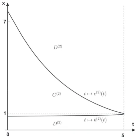
Theorem 3.8. There exist two functions b(2), c(2) : [0, Tδ] → (0,∞] such that 0 < b(2)(t) < K < c(2)(t)≤ ∞ and Ct(2) = (b(2)(t), c(2)(t)) for all t∈[0, Tδ]. Moreover b(2)(t)≥b(1)(t) for all t∈[0, Tδ], t7→b(2)(t) is increasing and t7→c(2)(t) is decreasing on [0, Tδ] with
lim
t↑Tδ
b(2)(t) = lim
t↑Tδ
c(2)(t) =K. (3.22)
Proof. The proof of existence is provided in 3 steps.
Step 1. First we show that it is not optimal to stop at x= K. To accomplish that we use arguments inspired by [26]. Fixε >0, set τε= inf{u≥0 :XuK ∈/ (K−ε, K+ε)}, taket∈[0, Tδ]
and denotes=Tδ−tthen by (3.10) and (3.11) we have that
V(2)(t, K)−G(t, K) (3.23)
≥Ee−rτε∧sG(t+τ
ε∧s, XτKε∧s)−G(t, K)
= 1 2E
Z τε∧s
0
e−rudLKu(XK)−rKE
Z τε∧s
0
e−ru I(XuK ≤K) +f(t+u, XuK) du
≥ 1
2E
Z τε∧s
0
e−rudLKu(XK)−C1E(τε∧s)
for some constant C1 > 0. The integral involving the local time can be estimated by using
Itˆo-Tanaka’s formula as follows
E
Z τε∧s
0
e−rudLKu(XK) (3.24)
=Ee−r(τε∧s)|XK
τε∧s−K| −rKE Z τε∧s
0
e−rusign(XuK−K)du
≥Ee−r(τε∧s)|XK
τε∧s−K| −C2E(τε∧s)
withC2=rK. Since|XτKε∧s−K| ≤εit is not hard to see that for any 0< p <1 we have
e−r(τε∧s)|XK
τε∧s−K| ≥e
−rp(τε∧s)|X
K
τε∧s−K|
p
εp e−
r(τε∧s)|XK
τε∧s−K|
then by taking the expectation and using the integral version of (2.1) we get
Ee−r(τε∧s)|XK
τε∧s−K| ≥
1
εpE
e−rτε∧s(XτK
ε∧s−K)
1+p
= 1
εpE rK
Z τε∧s
0
e−rudu+σ Z τε∧s
0
e−ruXuKdBu
1+p .
to obtain
Ee−rτε∧s|XK
τε∧s−K| ≥
1
εp2p+1E
σ
Z τε∧s
0
e−ruXuKdBu
1+p −ε1pE
rK
Z τε∧s
0
e−rudu
1+p
(3.25)
≥C4E
σ
2
Z τε∧s
0
e−2ru(XuK)2du
(1+p)/2
−C3E(τε∧s)1+p
≥C4C5E(τε∧s)(1+p)/2−C3E(τε∧s)1+p
for some constants C3 =C3(ε, p), C4 =C4(ε, p), C5 =C5(ε.p) >0. Since we are interested in
the limit asTδ−t→0 we takes <1, and combining (3.23), (3.24) and (3.25) we get
V(2)(t, K)−G(t, K)≥C4C5E(τε∧s)(1+p)/2−(C1+C2+C3)E(τε∧s) (3.26)
for any t ∈ [0, Tδ) such that s = Tδ−t < 1. Since p+1 < 2 it follows from (3.26) by letting s ↓ 0 that there exists t∗ < T
δ such that V(2)(t, K) > G(t, K) for all t ∈ (t∗, Tδ). Therefore
(t, K)∈Ct(2)for allt∈(t∗, T
δ) and sincet7→Ct(2) is decreasing (cf. Proposition 3.6) this implies
(t, K) ∈ Ct(2) for all t ∈ [0, Tδ), i.e. it is never optimal to stop when the underlying price X
equals the strikeK.
Step 2. Now we study the portion ofD(2) above the strike K and show that it is not empty. For that we argue by contradiction and we assume that there are no points in the stopping region above K. Take ε > 0, x ≥ K + 2ε and t ∈ [0, Tδ) and we denote τ = τ∗(t, x) the
optimal stopping time forV(2)(t, x). As before we sets=Tδ−tto simplify notation and define σε:= inf{u≥0 : Xux≤K+ε} ∧Tδ. Then by (3.10) and (3.11) we get
V(2)(t, x)−G(t, x)
=Ee−rτG(t+τ, Xτx)−G(t, x)
≤ −rKE
Z τ
0
e−ruf(t+u, Xux)du+1 2E
Z τ
0
e−rudLKu(Xx)
≤ −rKE
h
I(τ < s)
Z τ
0
e−ruf(t+u, Xux)dui−rKE
h
I(τ =s)
Z s
0
e−ruf(t+u, Xux)dui
+1 2E
h
I(σε< τ) Z τ
σε
e−rudLK u (Xx)
i
=−rKEh
Z s
0
e−ruf(t+u, Xux)dui+rKEhI(τ < s)
Z s
τ
e−ruf(t+u, Xux)dui
+1 2E
h
I(σε< τ) Z τ
σε
e−rudLKu (Xx)i
where we have used the fact that foru≤σεthe local timeLKu(Xx) is zero. Since we are assuming
that it is never optimal to stop above K then it must be
τ < s ⊂
σε < s . Obviously we
also have
σε< τ ⊂σε< s and hence
V(2)(t, x)−G(t, x) (3.27)
≤ −rKEh
Z s
0
e−ruf(t+u, Xux)dui
+E
h
I(σε< s)
rK Z s
τ
e−ruf(t+u, Xux)du+1 2
Z s
σε
e−rudLKu(Xx)i
≤ −rKE
hZ s
0
e−ruf(t+u, Xux)dui
+rKsP(σε< s) +
1 2E
I(σε< s)E
Z σε∨s
σε
e−rudLKu(Xx) Fσε
where we have used 0≤f ≤1 (cf. (3.8)) and the fact that I(σε< s is Fσε-measurable. From
Lemma 3.7 withσ=σε and τ =σε∨sand by the martingale property of (e−rtXtx)t≥0 we get
E
hZ σε∨s
σε
e−rudLKu(Xx) Fσε
i
(3.28)
≤2K+Ee−r(σε∨s)Xx
σε∨s Fσε
−e−rσεXx
σε +rKE
I(σε< s) Z s
σε
e−rtdt ≤3K.
Combining (3.27) and (3.28) we finally obtain
V(2)(t, x)−G(t, x)≤ −rKEh
Z s
0
e−ruf(t+u, Xux)dui+ 32K+rKs
P(σε< s). (3.29)
To estimate P σε < s it is convenient to set α := ln
x K+ε
, Yt := σBt+ (r−σ2/2)t and Zt:=−σBt+c twith c:=r+σ2/2. Notice that Yt≥ −Zt fort∈[0, Tδ] and hence
P(σε< s) =P
inf
0≤u≤sX x
u ≤K+ε
=P inf
0≤u≤sYu ≤ −α
(3.30)
≤P
inf
0≤u≤s−Zu ≤ −α
=P
sup
0≤u≤s
Zu ≥α
≤P
sup
0≤u≤s Zu
≥α
where we also recall that x≥K+2εand hence α >0. We now use Markov inequality, Doob’s inequality and BDG inequality to estimate the last expression in (3.30) and it follows that for any p >1
P
sup
0≤u≤s Zu
≥α
≤α1pE sup
0≤u≤s Zu p ≤ 2 p−1
αp
csp+σpE sup
0≤u≤s Bu
p
≤C1 sp+sp/2
(3.31)
with suitableC1=C1(p, ε, x)>0. Collecting (3.29) and (3.31) we get
V(2)(t, x)−G(t, x)≤sC2(sp+sp/2)+C3 sp−1+sp/2−1−rKE
h1 s
Z s
0
e−ruf(t+u, Xux)dui
(3.32)
for suitableC2 =C2(p, ε, x)>and C3=C3(p, ε, x)>0. We takep >2 and observe that in the
limit ass↓0 we get
−rKEh1
s Z s
0
e−ruf(t+u, Xux)dui+C2(sp+sp/2)+C3 sp−1+sp/2−1
→ −rKf(Tδ, x) (3.33)
and therefore the negative term in (3.32) dominates sincef(Tδ, x)>0 for all x∈(0,∞). From
(3.32) and (3.33) we get a contradiction and by arbitrariness ofεwe conclude that for anyx > K
there must bet < Tδ large enough and such that (t, x)∈D(2).
We show now that (t, x) ∈ D(2) with x > K implies (t, y) ∈ D(2) for any y > x. Take
y > x > K and assume (t, y)∈C(2). Setτ =τ∗(t, y) optimal for V(2)(t, y) defined as in (3.14)
and notice that the horizontal segment [t, Tδ]× {x} belongs to D(2) by Proposition 3.6. Then
the process (t+s, Xsy)s∈[0,Tδ−t] cannot hit the horizontal segment [t, Tδ]× {K} without entering
into the stopping set. Hence by (3.10) and (3.11) we have
V(2)(t, y) =Ee−rτG(t+τ, Xτy) =G(t, y)−rKE
hZ τ
0
e−rsf(t+s, Xsy)dsi≤G(t, y),
Dt(2)∩(K,∞) = [c(2)(t),∞) with the convention that if c(2)(t) = +∞ the set is empty. We
remark that for now we have only proven thatc(2)(t)<+∞fort < Tδ suitably large. Finiteness
ofc(2) will be provided in Proposition 3.10 below.
Step 3. Now let us consider the set{(t, x)∈[0, Tδ)×(0, K]}. From Proposition 3.5 it follows
that for each t∈[0, Tδ) the setD(2)t ∩(0, K) is not empty. Moreover by using arguments as in
step 2 above one can prove that for anyx < K there exists t < Tδ such that (t, x) ∈D(2), and
that x ∈ D(2)t =⇒ y ∈D(2)t for 0 < y ≤x ≤K. The latter implies that for each t ∈[0, Tδ)
there exists a unique pointb(2)(t)∈(0, K) such thatD(2)
t ∩(0, K) = (0, b(2)(t)].
Steps 1, 2 and 3 above imply that Ct(2) = b(2)(t), c(2)(t)
for allt∈[0, Tδ) and for suitable
functionsb(2), c(2) : [0, Tδ)→(0,∞]. The fact thatb(2)(t)≥b(1)(t) is an obvious consequence of
Proposition 3.5. On the other hand Proposition 3.6 implies thatt7→b(2)(t) is increasing whereas
t7→ c(2)(t) is decreasing so that their left-limits always exist. Since limt↑Tδc
(2)(t)≥K and for
any x > K there exists t < Tδ with (t, x) ∈ D(2) (see step 2 above), then limt↑Tδc
(2)(t) = K.
From a similar argument and step 3 above we also obtain limt↑Tδb
(2)(t) =K.
Remark 3.9. 1. The existence of an upper boundary is a key consequence of the constraints imposed by the structure of Sn
t,T in (1.2) (see also the discussion at the beginning of Section
2.2) and it nicely reflects the time value of the early exercise feature of the option. Indeed for t < Tδ the holder may find profitable to use the first right even if Xt> K (i.e. the put part of
the immediate exercise payoff is zero) in order to maintain the opportunity of early exercising the remaining put option with maturity atT (after the refracting period).
If for some t < Tδ the underlying priceXtis too large, the holder does not believe that it will
fall belowK prior toTδ. In this case delaying the exercise of the first right is likely to produce a
null put payoff while at the same time reducing the value of the subsequent early exercise right. On the other hand, by using immediately the first right, the option holder will maximise at least the opportunities of an early exercise of the second option. It then becomes intuitively clear that while the holder of a standard American put option has nothing to lose in waiting as long asX stays above K, for our swing contract things are different: waiting always costs to the holder in terms of the early exercises of future rights. Hence when the immediate put payoff of the first option is way too much “out of the money” it is better to get rid of it!
2. We observe that it is P-almost surely optimal to exercise the first right of the swing option strictly before the maturity Tδ since
P(Xtx∈Ct(2)for all t∈[0, Tδ])≤P(XTxδ =K) = 0.
3. It is known that as r → 0 the premium of early exercise for the American option vanishes thus meaning that b(1) ≡ 0 for r = 0. Analogously, for r = 0 there is no incentive in using
the first right of the swing contract with n = 2 at any time prior to Tδ so that b(2) ≡ 0 and c(2) ≡+∞. This fact will be clearly embodied in the pricing formula for V(2) in Theorem 3.13 below.
In Theorem 3.8 we have proven thatc(2)(t)<∞for alltsmaller than but “sufficiently close”
toTδ. We now aim at strengthening this statement by proving thatc(2)is indeed finite on [0, Tδ].
Proposition 3.10. For all t∈[0, Tδ]the upper boundary c(2) is finite, i.e.
sup
t∈[0,Tδ]
c(2)(t)<+∞. (3.34)
Step 1. Let us assume that (3.34) is violated and denote t0 := sup{t ∈ [0, Tδ] : c(2)(t) =
+∞}. Consider for now the caset0 >0 and note that sincet7→c(2)(t) is decreasing by Theorem
3.8 then c(2)(t) = +∞ for all t∈[0, t0). The functionc(2) is right-continuous on (t0, Tδ], in fact
for anyt∈(t0, Tδ] we take tn↓t as n→ ∞ and the sequence (tn, c(2)(tn))∈D(2) converges to
(t, c(2)(t+)), withc(2)(t+) := lim
s↓tc(2)(s). Since D(2) is closed it must also be (t, c(2)(t))∈D(2)
and c(2)(t+)≥c(2)(t) by Theorem 3.8, hencec(2)(t+) =c(2)(t) by monotonicity. For x∈(K,+∞) we define the right-continuous inverse ofc(2) by tc(x) := sup
t∈[0, Tδ] : c(2)(t) > x and observe that t
c(x) ≥ t0. Fix ε > 0 such that ε < δ∧t0, then there exists
x=x(ε)> K such that tc(x)−t0 ≤ε/2 for allx ≥x and we denote θ=θ(x) := infu ≥0 :
Xux≤x ∧Tδ. In particular we note that if c(2)(t0+) =c(2)(t0)<+∞ we havetc(x) =t0 for all
x > c(2)(t0). We fixt=t0−ε/2, take x > xand set τ =τ∗(t, x) the optimal stopping time for
V(2)(t, x) (cf. (3.14)).
From (3.11) we get
V(2)(t, x)−G(t, x) =Ee−rτG(t+τ, Xx
τ)−G(t, x)
≤Eh−rK Z τ
0
e−rsf(t+s, Xsx)ds+1 2
Z τ
0
e−rsdLKs (Xx)i
≤ −rKE
h
I(τ ≤θ)
Z τ
0
e−rsf(t+s, Xsx)dsi+E
h
I(τ > θ)1 2
Z τ
θ
e−rsdLKs (Xx)i
where we have used that LKs (Xx) = 0 for s≤ θ. Since c(2)(t) = +∞ for t∈ [t0−ε/2, t0) and
the boundary is decreasing then it must be{τ ≤θ} ⊆ {τ ≥ε/2}. Hence we obtain
V(2)(t, x)−G(t, x) (3.35)
≤ −rKE
hZ ε/2
0
e−rsf(t+s, Xsx)dsi
+EhI(τ > θ)1 2
Z τ
θ
e−rsdLKs (Xx)+rK Z ε/2
0
e−rsf(t+s, Xsx)dsi
≤ −rKEh
Z ε/2
0
e−rsf(t+s, Xsx)dsi+1 2E
I(τ > θ)Eh
Z τ∨θ
θ
e−rsdLKs (Xx)
Fθ
i
+rKε
2P(τ > θ)
where in the last inequality we have also used that 0 ≤ f ≤ 1 on [0, Tδ]×(0,∞). We now
estimate separately the two positive terms in the last expression of (3.35). For the one involving the local time we argue as in (3.28), i.e. we use Lemma 3.7 and the martingale property of the discounted price to get
E
Z τ∨θ
θ
e−rsdLK s (Xx)
Fθ
≤3K.
Then for a suitable constantC1 >0 independent ofx we get
E
I(τ > θ)E
Z τ∨θ
θ
e−rsdLKs (Xx) Fθ
+rKε
2P(τ > θ)≤C1P(τ > θ). (3.36) Observe now that on
τ > θ the process X started at time t=t0−ε/2 from x > xmust hit
x prior to timet0+ε/2, hence, forc=r+σ2/2, we obtain
P(τ > θ)≤P inf
0≤t≤εX x t < x
≤P
inf
0≤t≤εBt<
1
σ
lnx
x +c ε
Introduce another Brownian motion by taking W := −B, then from (3.37) and the reflection principle we find
P(τ > θ)≤P
sup
0≤t≤ε
Wt>−
1
σ
lnx
x +c ε
= 2P
Wε >−
1
σ
lnx
x +c ε
(3.38)
=2h1−Φσ√1
ε ln(x/ x)−c ε i
= 2Φσ√1
ε ln(x/x) +c ε
with Φ(y) := 1/√2πRy −∞e−z
2/2
dz fory ∈IR and where we have used Φ(y) = 1−Φ(−y),y ∈IR. Going back to (3.35) we aim at estimating the first term in the last expression. For that we use Markov property to obtain
Ef(t+s, Xsx) =e−rδEP Xsx+δ≤b(1)(t+s+δ)
Fs =e−rδP
Xsx+δ≤b(1)(t+s+δ)
(3.39)
withs∈[0, ε/2]. For allx > xand s∈[0, ε/2] and denotingα :=b(1)(t+δ), the expectation in (3.39) is bounded from below by recalling thatb(1) is increasing, namely
Ef(t+s, Xsx)≥e−rδP(Xsx+δ≤α)≥e−rδP
Bs+δ≤
1
σ
ln(α/x)−c(δ+ε/2)
(3.40)
=e−rδΦσ√1 δ+s
ln(α/ x)−c(δ+ε/2)
≥e−rδΦ 1
σ√δ
ln(α/ x)−c(δ+ε/2)
=: ˆF(x)
where in the last inequality we have used that ln(α/ x) <0 and Φ is increasing. From (3.40), using Fubini’s theorem we get
Eh
Z ε/2
0
e−rsf(t+s, Xsx)dsi=
Z ε/2
0
e−rsEf(t+s, Xsx)ds≥ ε
2e
−rε/2Fˆ(x) (3.41)
forx > x. We now collect bounds (3.35), (3.36), (3.38) and (3.41) to obtain
V(2)(t, x)−G(t, x) (3.42)
≤2C1Φ
1
σ√ε ln(x/x) +c ε
−C2Φ
1
σ√δ
ln α/ x
−c(δ+ε/2)
whereC2 =C2(ε)>0 and independent of x. Sincet, x, ε are fixed withδ > ε, we take the limit
asx→ ∞ and it is not hard to verify by L’Hˆopital’s rule that
lim
x→∞
Φσ√1
ε ln(x/x) +c ε
Φ 1
σ√δ
ln α/ x
−c(δ+ε/2) =C3xlim→∞
ϕσ√1
ε ln(x/x) +c ε
ϕ 1 σ√δ
ln α/ x
−c(δ+ε/2)
=C4 lim
x→∞x
βexp 1
σ2 1/δ−1/ε
lnx2
= 0
for suitable positive constantsβ >0,C3 and C4 and with ϕ:= Φ′ the standard normal density
function. Hence the negative term in (3.42) dominates for large values of x and we reach a contradiction. That impliesc(2)(t)<+∞ for all t∈(0, T
δ] by arbitrariness oft0.
Step 2. It remains to show that c(2)(0) <+∞ as well. In order to do so we recall Remark 2.1 and notice that V(2)(0, x;Tδ)−G(0, x;Tδ) = V(2)(λ, x;Tδ+λ)−G(λ, x;Tδ+λ) for λ >0.
Hence the arguments in step 1 may be applied with t0 =λand Tδ replaced by Tδ+λ, proving
3.1.3. Free-boundary problem for V(2) and continuity of the boundaries
To prepare the ground to the free-boundary problem for V(2) we begin by showing in the next proposition that the value function V(2) fulfills the so-called smooth-fit condition at both the
optimal boundariesb(2) andc(2).
Proposition 3.11. For all t∈ [0, Tδ) the map x7→ V(2)(t, x) is C1 across the optimal
bound-aries, i.e.
Vx(2)(t, b(2)(t)+) =Gx(t, b(2)(t)) (3.43)
Vx(2)(t, c(2)(t)−) =Gx(t, c(2)(t)). (3.44)
Proof. We provide a full proof only for (3.44) as the one for (3.43) can be obtained in a similar way. Fix 0≤t < Tδ and setx0:=c(2)(t). It is clear that for arbitrary ε >0 it hods
V(2)(t, x
0)−V(2)(t, x0−ε)
ε ≤
G(t, x0)−G(t, x0−ε)
ε
and hence
lim sup
ε→0
V(2)(t, x0)−V(2)(t, x0−ε)
ε ≤Gx(t, x0). (3.45)
To prove the reverse inequality, we denoteτε=τ∗(t, x0−ε) which is the optimal stopping time
forV(2)(t, x
0−ε). Then using the law of iterated logarithm at zero for Brownian motion and
the fact that t7→c(2)(t) is decreasing we obtainτε → 0 asε→ 0,P-a.s. An application of the
mean value theorem gives
1
ε
V(2)(t, x0)−V(2)(t, x0−ε)
≥ 1 εE
h e−rτε
G(t+τε, Xτxε0)−G(t+τε, X
x0−ε
τε ) i
≥ 1 εE
h e−rτεG
x(t+τε, ξ) Xτxε0 −X
x0−ε
τε i
= Ehe−rτεG
x(t+τε, ξ)Xτ1ε i
with ξ(ω) ∈ [Xx0−ε
τε (ω), X
x0
τε(ω)] for all ω ∈ Ω. Thus recalling that Gx is bounded (cf. (3.15))
and Xτ1ε →1 P-a.s. as ε→0, using dominated convergence theorem we obtain
lim inf
ε→0
V(2)(t, x
0)−V(2)(t, x0−ε)
ε ≥Gx(t, x0). (3.46)
Finally combining (3.45) and (3.46), and using that V(t, ·) is convex (see Proposition 3.4) we obtain (3.44).
Standard arguments based on the strong Markov property and continuity of V(2)(see [25, Sec. 7], p. 131) imply thatV(2)∈C1,2 inside the continuation setC(2)and it solves the following
free-boundary problem
Vt(2)+ILXV(2)−rV(2)= 0 inC(2) (3.47)
V(2)(t, b(2)(t)) =G(t, b(2)(t)) fort∈[0, Tδ] (3.48)
V(2)(t, c(2)(t)) =G(t, c(2)(t)) fort∈[0, Tδ] (3.49)
Vx(2)(t, b(2)(t)+) =Gx(t, b(2)(t)) fort∈[0, Tδ) (3.50)
Vx(2)(t, c(2)(t)−) =Gx(t, c(2)(t)) fort∈[0, Tδ) (3.51)
Thanks to our results of the previous section the continuation setC(2)and the stopping setD(2)
are given by
C(2) ={(t, x)∈[0, Tδ)×(0,∞) :b(2)(t)< x < c(2)(t)} (3.53)
D(2) ={(t, x)∈[0, Tδ]×(0,∞) :x≤b(2)(t) orx≥c(2)(t)}. (3.54)
Notice that (3.48)–(3.52) follow by the definition ofb(2) and c(2) and by Proposition 3.11. For
the unfamiliar reader we give in appendix the standard proof of (3.47).
We now proceed to prove that the boundaries b(2) and c(2) are indeed continuous functions
of time and follow the approach proposed in [10].
Theorem 3.12. The optimal boundaries b(2) and c(2) are continuous on[0, T
δ].
Proof. The proof is provided in 3 steps.
Step 1. By monotonicity and boundedness ofb(2) and c(2) we obtain their right-continuity
(see the first paragraph of step 1 in the proof of Proposition 3.10).
Step 2. Now we prove that b(2) is also left-continuous. Assume that there exists t0 ∈(0, Tδ]
such that b(2)(t
0−) < b(2)(t0) where b(2)(t0−) denotes the left-limit of b(2) att0. Take x1 < x2
such that b(2)(t0−) < x1 < x2 < b(2)(t0) and h > 0 such that t0 > h, then define the domain
D:= (t0−h, t0)×(x1, x2) and denote by∂PDits parabolic boundary formed by the horizontal
segments [t0−h, t0]× {xi}withi= 1,2 and by the vertical one{t0} ×(x1, x2). Recall that both
G and V(2) belong to C1,2(D) and it follows from (3.10), (3.47) and (3.48) that u := V(2)−G
is such that u∈C1,2(D)∩C(D) and it solves the boundary value problem
ut+ILXu−ru=−H on Dwith u= 0 on ∂PD. (3.55)
Denote byC∞
c (a, b) the set of continuous functions which are differentiable infinitely many times
with continuous derivatives and compact support on (a, b). Takeϕ∈C∞
c (x1, x2) such thatϕ≥0
and Rx2
x1 ϕ(x)dx= 1. Multiplying (3.55) byϕand integrating by parts we obtain
Z x2
x1
ϕ(x)ut(t, x)dx=− Z x2
x1
u(t, x) (IL∗Xϕ(x)−rϕ(x))dx− Z x2
x1
H(t, x)ϕ(x)dx (3.56)
fort∈(t0−h, t0) and with IL∗X denoting the formal adjoint of ILX. Since ut≤0 in Dby (3.20)
in the proof of Proposition 3.6, the left-hand side of (3.56) is negative. Then taking limits as
t→t0 and by using dominated convergence theorem we find
0≥ −
Z x2
x1
u(t0, x) (IL∗Xϕ(x)−rϕ(x))dx− Z x2
x1
H(t0, x)ϕ(x)dx (3.57)
=− Z x2
x1
H(t0, x)ϕ(x)dx
where we have used thatu(t0, x) = 0 forx∈(x1, x2) by (3.55). We now observe that H(t0, x)<
−ℓforx∈(x1, x2) and a suitable ℓ >0 by (3.10), therefore (3.57) leads to a contradiction and
it must beb(2)(t
0−) =b(2)(t0).
Step 3. To prove thatc(2) is left-continuous we can use arguments that follow the very same
3.1.4. The EEP representation of the option’s value and equations for the boundaries
Finally we are able to find an early-exercise premium (EEP) representation forV(2) of problem (3.5) and a system of coupled integral equations for the free-boundaries b(2) and c(2). The
following functions will be needed in the next theorem:
J(t, x) :=ExG(Tδ, XTδ−t), (3.58) K(b(1), b(2), c(2);x, t, s) :=Px(Xs≤b(2)(t+s)) (3.59)
+e−rδPx Xs≤b(2)(t+s), Xs+δ≤b(1)(t+s+δ)
+e−rδPx Xs≥c(2)(t+s), Xs+δ≤b(1)(t+s+δ)
.
Theorem 3.13. The value function V(2) of (3.5)has the following representation
V(2)(t, x) = e−r(Tδ−t)J(t, x) +rK Z Tδ−t
0
e−rsK(b(1), b(2), c(2);x, t, s)ds (3.60)
fort∈[0, Tδ]andx∈(0,∞). The optimal stopping boundaries b(2) andc(2) of (3.53)and (3.54)
are the unique couple of continuous functions solving the system of coupled nonlinear integral equations
G(t, b(2)(t)) = e−r(Tδ−t)J(t, b(2)(t)) +rK Z Tδ−t
0
e−rsK(b(1), b(2), c(2);b(2)(t), t, s)ds (3.61)
G(t, c(2)(t)) = e−r(Tδ−t)J(t, c(2)(t)) +rK Z Tδ−t
0
e−rsK(b(1), b(2), c(2);c(2)(t), t, s)ds (3.62)
withb(2)(T
δ) =c(2)(Tδ) =K and b(2)(t)≤K ≤c(2)(t) for t∈[0, Tδ].
Proof. Step 1 - Existence. Here we prove that b(2) and c(2) solve (3.61)–(3.62). We start by recalling that the following conditions hold: (i) V(2) is C1,2 separately in C(2) and D(2) and
Vt(2)+ILXV(2)−rV(2) is locally bounded on C(2)∪D(2) (cf. (3.47)–(3.52) and (3.10)); (ii) b(2)
and c(2) are of bounded variation due to monotonicity; (iii) x 7→ V(2)(t, x) is convex (recall proof of Proposition 3.4); (iv) t7→Vx(2)(t, b(2)(t)±) and t7→ Vx(2)(t, c(2)(t)±) are continuous for t∈[0, Tδ) by (3.50) and (3.51). Hence for any (t, x) ∈[0, Tδ]×(0,∞) and s∈[0, Tδ−t] we can
apply the local time-space formula on curves of [24] to obtain
e−rsV(2)(t+s, Xsx) (3.63)
=V(2)(t, x) +Mu
+
Z s
0
e−ru(Vt(2)+ILXV(2)−rV(2))(t+u, Xux)I Xux6={b(2)(t+u), c(2)(t+u)}
du
=V(2)(t, x) +Mu+ Z s
0
e−ruH(t+u, Xux)hI Xux< b(2)(t+u)
+I Xux> c(2)(t+u)i du
=V(2)(t, x) +Mu−rK Z s
0
e−ru 1 +f(t+u, Xux)
I Xux< b(2)(t+u) du
−rK Z s
0
e−ruf(t+u, Xux)I Xux > c(2)(t+u) du
where we used (3.10), (3.47) and smooth-fit conditions (3.50)-(3.51) and whereM = (Mu)u≥0
is a real martingale. Recall that the law of Xx
u is absolutely continuous with respect to the
Lebesgue measure for allu >0, then from strong Markov property and (3.8) we deduce
f(t+u, Xux)I Xux< b(2)(t+u)
=P Xux+δ ≤b(1)(t+u+δ) Fu
I Xux< b(2)(t+u)
(3.64)
=P Xux+δ ≤b(1)(t+u+δ), Xux ≤b(2)(t+u) Fu
Figure 1. A computer drawing of the optimal exercise boundaries t7→b(2)(t) and t7→c(2)(t) in the case K= 1, r= 0.05 (annual),σ= 0.2 (annual),T = 6 months, δ= 1 month.
and analogously we have that
f(t+u, Xux)I Xux> c(2)(t+u)
=P Xux+δ≤b(1)(t+u+δ), Xux≥c(2)(t+u) Fu
. (3.65)
In (3.63) we let s=Tδ−t, take the expectationE, use (3.64)-(3.65) and the optional sampling
theorem for M, then after rearranging terms and noting that V(2)(Tδ, x) = G(Tδ, x) for all x > 0, we get (3.60). The system of coupled integral equations (3.61)-(3.62) is obtained by simply puttingx=b(2)(t) andx=c(2)(t) into (3.60) and using (3.48)-(3.49).
Step 2 - Uniqueness. Now we show uniqueness of the solution pair to the system (3.61)-(3.62). The proof is divided in five steps and it is based on arguments similar to those employed in [11] and originally derived in [23].
Step 2.1. Let b : [0, Tδ] → (0,∞) and c : [0, Tδ] → (0,∞) be another solution pair to the
system (3.61)-(3.62) such that b and c are continuous and b(t) ≤ K ≤ c(t) for all t ∈ [0, Tδ].
We will show that thesebandcmust be equal to the optimal stopping boundariesb(2) and c(2), respectively.
We define a continuous functionUb,c : [0, T
δ]×(0,∞)→IR by
Ub,c(t, x) :=e−r(Tδ−t)EG(T
δ, XTxδ−t)
−E
Z Tδ−t
0
e−ruH(t+u, Xux)I(Xux≤b(t+u) or Xux ≥c(t+u))du.
Observe that since b and c solve the system (3.61)-(3.62) then Ub,c(t, b(t)) = G(t, b(t)) and
Ub,c(t, c(t)) =G(t, c(t)) for all t∈[0, T
δ]. Notice also that the Markov property of X gives
e−rsUb,c(t+s, Xsx)−
Z s
0
e−ruH(t+u, Xux)I(Xux ≤b(t+u) orXux≥c(t+u))du (3.66)
fors∈[0, Tδ−t] and with (Ns)0≤s≤Tδ−t aP-martingale.
Step 2.2. We now show that Ub,c(t, x) = G(t, x) for x ∈ (0, b(t)]∪[c(t),∞) and t∈ [0, T δ].
Forx∈(0, b(t)]∪[c(t),∞) witht∈[0, Tδ] given and fixed, consider the stopping time
σb,c=σb,c(t, x) = inf {0≤s≤Tδ−t:b(t+s)≤Xsx≤c(t+s) }. (3.67)
Using thatUb,c(t, b(t)) =G(t, b(t)) andUb,c(t, c(t)) =G(t, c(t)) for allt∈[0, Tδ) andUb,c(Tδ, x) = G(Tδ, x) for all x >0, we get Ub,c(t+σb,c, Xσxb,c) =G(t+σb,c, X
x
σb,c) P-a.s. by continuity ofU
b,c.
Hence from (3.11) and (3.66) using the optional sampling theorem and noting thatLKu (Xx) = 0 foru≤σb,c we find
Ub,c(t, x) =Ee−rσb,cUb,c(t+σ
b,c, Xσxb,c)
−E
Z σb,c
0
e−ruH(t+u, Xux)I(Xux ≤b(t+u) orXux ≥c(t+u))du
=Ee−rσb,cG(t+σ
b,c, Xσxb,c)−E Z σb,c
0
e−ruH(t+u, Xux)du=G(t, x)
sinceXux∈(0, b(t+u))∪(c(t+u),∞) for all u∈[0, σb,c).
Step 2.3. Next we prove that Ub,c(t, x) ≤V(2)(t, x) for all (t, x) ∈[0, T
δ]×(0,∞). For this
consider the stopping time
τb,c=τb,c(t, x) = inf { 0≤s≤Tδ−t:Xsx≤b(t+s) orXsx≥c(t+s) }
with (t, x) ∈[0, Tδ]×(0,∞) given and fixed. Again arguments as those following (3.67) above
show that Ub,c(t+τ
b,c, Xτxb,c) = G(t+τb,c, X
x
τb,c) P-a.s. Then taking s=τb,c in (3.66) and using
the optional sampling theorem, we get
Ub,c(t, x) =Ee−rτb,cUb,c(t+τ
b,c, Xτxb,c) =Ee
−rτb,cG(t+τ
b,c, Xτxb,c)≤V
(2)(t, x).
Step 2.4. In order to compare the couples (b, c) and (b(2), c(2)) we initially prove thatb(t)≥
b(2)(t) and c(t)≤c(2)(t) fort ∈[0, T
δ]. For this, suppose that there exists t∈[0, Tδ) such that c(t)> c(2)(t), take a pointx∈[c(t),∞) and consider the stopping time
σ=σ(t, x) = inf { 0≤s≤Tδ−t:b(2)(t+s)≤Xsx ≤c(2)(t+s) }.
Settings=σ in (3.63) and (3.66) and using the optional sampling theorem, we get
Ee−rσV(2)(t+σ, Xσx) =V(2)(t, x) +E
Z σ
0
e−ruH(t+u, Xux)du (3.68)
Ee−rσUb,c(t+σ, Xσx) =Ub,c(t, x) (3.69)
+E
Z σ
0
e−ruH(t+u, Xux)I Xux ≤b(t+u) orXux≥c(t+u) du.
SinceUb,c ≤V(2) andV(2)(t, x) =Ub,c(t, x) =G(t, x) forx∈[c(t),∞), it follows by subtracting
(3.69) from (3.68) that
E
Z σ
0
e−ruH(t+u, Xux)I b(t+u)≤Xux≤c(t+u)
du≥0. (3.70)
The function H is always strictly negative and by the continuity of c(2) and c it must be