Analysis of spatial emission structures in vertical-cavity surface-emitting lasers with feedback
from a volume Bragg grating
Y. Noblet*and T. Ackemann†
SUPA, Department of Physics, University of Strathclyde, 107 Rottenrow, Glasgow G4 0NG, Scotland, UK (Received 27 January 2012; published 10 May 2012)
We investigate the spatial and spectral properties of broad-area vertical-cavity surface-emitting lasers with frequency-selective feedback by a volume Bragg grating. We demonstrate wavelength locking similar to the case of edge emitters but the spatial mode selection is different from the latter. On-axis spatial solitons obtained at threshold give way to off-axis extended lasing states beyond threshold. The investigations focus on a self-imaging external cavity. We analyze how deviations from the self-imaging condition affect the pattern formation and a certain robustness of the phenomena is demonstrated.
DOI:10.1103/PhysRevA.85.053812 PACS number(s): 42.55.Px, 42.60.Jf, 42.65.Sf, 42.60.Da
I. INTRODUCTION
Volume Bragg gratings (VBGs) are compact, narrow-band frequency filters which prove to be of increasing use in photonics. One particular application is the wavelength control of edge-emitting laser diodes (EELs), where they can stabilize the emission wavelength very effectively against the redshift connected with an increase in ambient temperature or with ohmic heating due to increasing current [1–3]. In addition, the spectral and spatial brightness of broad-area EELs can be reduced significantly by the feedback from a VBG [1,2]. Commercial versions are referred to as “wavelength lockers” or “power lockers.”
Frequency-selective feedback was proposed and demon-strated to provide some control of transverse modes also for vertical-cavity surface-emitting lasers (VCSELs), both for medium-sized devices emitting Gaussian modes [4,5] and for broad-area devices emitting Fourier modes [6]. These investigations used diffraction gratings, and to our knowledge, the only investigations using VBGs were performed with a focus on the close-to-threshold region where bistable spatial solitons are formed [7,8]. In this work, we report experiments on how the solitons formed at threshold give way to spatially extended spatial structures and analyze their properties quantitatively. We discuss similarities to and differences from the edge-emitting case and to what extent VBGs are helpful to control spatial modes in a VCSEL. We focus on a specific setup of the external cavity close to a self-imaging situation and analyze how deviations from the self-imaging condition influence the pattern formation. Not only is the latter important for pattern formation as investigated in this paper and feedback experiments for modal control [4–6], but also there is recent interest in using self-imaging or close-to-self-imaging cavities to study large arrays of coupled lasers and coupled laser solitons [9–11]. Deviations from the self-imaging condition modify the strength of the coupling via the nonlocality introduced. Hence, a proper characterization and thorough understanding of cavity properties near a
self-*[email protected] †[email protected]
imaging situation are required when exploring synchronization dynamics and frequency and phase locking in these systems.
II. EXPERIMENTAL SETUP
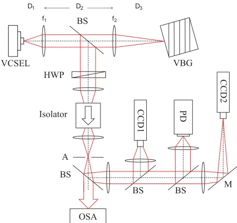
A schematic of the experimental setup is illustrated in Fig.1. The VCSEL used for this experiment is fabricated by Ulm Photonics and similar to the ones described in more detail in Refs. [6,7,12–14]. It is a large-aperture device, allowing for the formation of many transverse cavity modes of fairly high order, with a 200-μm-diameter circular oxide aperture providing optical and current guiding. Emission takes place through the n-doped Bragg reflector and through a transparent substrate (a so-called bottom emitter [13,14]). The laser has an emission wavelength of about 975 nm at room temperature. The VCSEL is tuned in temperature up to 70◦C so that the emission wavelength approaches the reflection peak of the VBG. The VBG has a reflection peak atλg=981.1 nm, with a reflection band width of 0.2-nm full-width at half-maximum (FWHM). At such a high temperature the free-running laser has a nearly infinite threshold and lasing only occurs because of the feedback from the VBG.
The VCSEL is coupled to the VBG via a self-imaging external cavity. Every point of the VCSEL is imaged at the same spatial position after each round-trip, therefore maintaining the high Fresnel number of the VCSEL cavity.
The VCSEL is collimated by anf1=8-mm-focal-length planoconvex aspheric lens. The second lens is an f2= 50-mm-focal-length planoconvex lens and is used to focus the light onto the VBG. This telescope setup gives a 6.25:1 magnification factor onto the VBG. This cavity has a round-trip frequency of 1.23 GHz, which corresponds to a round-trip time of 0.81 ns. The light is coupled out of the cavity using a glass plate [a beamsplitter with a front uncoated facet and a back antireflection-coated facet]. The reflection relies on Fresnel reflection and therefore is polarization dependent. The reflectivity is of the order of 10% for s-polarized light and 1% for p-polarized light.
FIG. 1. (Color online) Experimental setup. A, aperture; BS, beamsplitter; CCD1, CCD camera in the near-field image plane of the vertical-cavity surface-emitting laser (VCSEL); CCD2, CCD camera in the far-field image plane of the VCSEL; HWP, half-wave plate; M, mirror; OSA, optical spectrum analyzer; PD, photodiode; VBG, volume Bragg grating.
the Fourier plane of the gain region (far field). The emission spectrum is recorded with an optical spectrum analyzer. There is also a photodiode which measures the laser power.
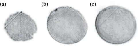
[image:2.608.49.292.68.297.2]The spontaneous emission is rather homogeneous below threshold [Fig.2(a)], but as the current increases the intensity becomes higher at the boundaries due to current crowding at the oxide aperture [14]. In spite of the large aperture, the device is still capable of lasing at low enough temperatures. The lower the temperature, the lower the current required to achieve lasing. Above threshold the laser starts to lase in a kind of whispering gallery mode (e.g., [15]) around the boundaries of the VCSEL [Fig.2(b)]. The gain is the highest there due to the current crowding previously observed, which leads to a lower threshold of this mode.
FIG. 2. Near-field intensity distribution of the VCSEL showing (a) spontaneous emission atI=200 mA (at a temperature of 70◦C) without feedback (this and all other images in this article depict the intensity on a linear gray scale, with black denoting high intensity); (b) the VCSEL without feedback, I=490 mA at T =16◦C; (c) the VCSEL with feedback from a plane mirror, whereI=185 mA atT =70◦C. Note that the slight nonhomogeneous behavior of the spontaneous emission (decrease in intensity from the upper left to the lower right) is due to the detection setup.
III. EXPERIMENTAL RESULTS A. Alignment of self-imaging cavity
As indicated, the cavity consists of two lenses forming an astronomical telescope. Thus the magnification factorM of this telescope is determined by the ratio of the two focal lengths. The position of the first lens,D1, is adjusted to provide the best collimation of the VCSEL output. The distance between the two intracavity lenses,D2, should bef1+f2for an afocal telescope, wheref1andf2are the two focal lengths of both lenses. In reality, this is difficult to adjust because the lenses are “thick;” i.e., D2 should refer to the distance between the principal planes, which is not easy to measure. In addition, there is no simple criterion for aligningD2just from observing images of the VCSEL output on a CCD camera. Therefore we started with an approximate placement given by the focal lengths of the lenses but validated and improved this as discussed in Sec.V. Taking dispersion data from the manufacturer into account, the nominally 8-mm collimation lens and the 50-mm focusing lens have an effective focal length of 8.07 and 50.79 mm, respectively, at 980 nm. The principal plane of a planoconvex lens (or a nearly planoconvex lens such as the aspheric lens) at the curved side should be directly at the tip. The intracavity beamsplitter makes the diffractive length about 0.8 mm shorter than the real length. Hence the distance between back (curved side) of the collimation lens and the front (curved side) of the focusing lens should be (8.07+50.79+0.8) mm=59.66 mm. In the setup, the distance from the front side of the mount of the collimation lens to the back of the mount holding the focusing lens (each adds 1 mm) is the only convenient distance to measure and was taken to representD2. The thickness of our lenses is 3.69 and 5.3 mm, respectively, for the collimation lens and the focusing lens. Therefore the self-imaging intracavity distance is esti-mated to be (59.66+3.69+1+5.3+1) mm=70.65 mm. Obviously, adjusting this distance only by measurement with a caliper will have an uncertainty of the order of 0.5 mm.
In order to confirm these considerations, another exper-iment has been set up to study the cavity in detail. It consists of the same telescope with the exact same optics (a collimation lens, a focusing lens, and a beamsplitter). A tunable laser is coupled into a single-mode fiber. The collimated output beam is then injected into the telescope from the side with the larger-focal-length lens. One should expect that the beam coming out of the telescope at the collimation lens has the smallest beam divergence if the intracavity distance is correct, and indeed the best collimation is found atD2=70.5 mm±0.2 mm, which is considered to be the accuracy of the distance measurement. This result matches the theoretically estimated distance of 70.65 mm within the uncertainties and is therefore used as the reference position. The data given in Figs.2(c)and3correspond to the optimized position.
[image:2.608.49.295.577.651.2]FIG. 3. Near-field intensity distribution of the VCSEL with feedback from a VBG at different currents. Left column,D3 at the self-imaging distance; center columns,D3too short or too large by 4 mm; right column, feedback with a plane mirror.
discussion around Eq. (4) below], but for self-imaging of intensity and phase profiles, the intracavity distance needs to equalf1+f2.
B. Feedback with a mirror
[image:3.608.52.292.631.712.2]For completeness, we study first the case of feedback with a plane mirror, i.e., without frequency selection. The laser starts at the quite low threshold of about 170 mA. The emission [Fig.2(c)] is characterized by a ring with fringes perpendicular to the aperture and this is very similar to what we observe in the free-running laser at lower temperatures. Obviously, this preference for the perimeter is again a gain effect due to the current crowding.
FIG. 4. Near-field intensity distribution of the VCSEL with feedback from a VBG (a), (b), and a plane mirror (c). (a), (c),I=450 mA; (b)I=550 mA.
FIG. 5. Far-field intensity distribution of the VCSEL with feed-back from a VBG at different currents. Left column, D3 at the self-imaging distance; center columns,D3too short or too large by 4 mm; right column, feedback with a plane mirror.
If the current is increased, the inner part of the lasing aperture starts to lase also, but a certain preference for the perimeter remains (Fig. 3; upper image, right column). A blowup of a characteristic structure is shown in Fig.4(c). If the current is increased further, the output power increases further but the spatial structure stays essentially the same (Fig.3; lower images, right column). The emission in the far field (Fig.5; right column) is quite broad, with a disk-shaped structure on the axis surrounded by a faint halo. At the transition between the center and the halo, one wave number is somewhat enhanced, leading to a ring. This wave number is probably favored by the detuning between the frequency of the gain maximum and the longitudinal cavity resonance as discussed before for free-running devices of this kind [15].
C. Feedback with the VBG
quite similar to those obtained with a plane mirror, i.e., fine waves at a high spatial frequency filling up the whole aperture of the device. However, there is the important difference that the length scale now depends on current: as a comparison of the blowups in Fig.4(a)vs Fig.4(b)shows, the wavelength of these waves decreases with increasing current.
This feature can be much better investigated in far-field images. The sequence depicted in the leftmost column in Fig.5 illustrates that the emission is very much dominated by a single ring with negligible background, i.e., only a single transverse wave number is lasing. The solitons start to emit on axis and the wave number increases monotonically with increasing current. We do a quantitative investigation at the end of Sec.IV.
If the distanceD3 is changed away from the self-imaging condition, the far-field images do not show a significant change except for quantitative corrections to the wave number (analyzed in more detail in Sec.V), but the near-field images do. For a longer cavity (+4 mm) we observe a “defocusing” effect, i.e., the emission is shifting toward the boundaries of the aperture, especially at high currents. Inversely, for a too short cavity,−4 mm, the pattern seems to be “focused,” i.e., it contracts toward the center of the device.
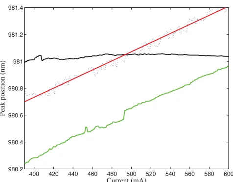
Finally, Fig. 6 gives an indication of the change in emission wavelength with increasing current. The free-running laser shows an approximately linear increase, at a rate of 0.0035 nm/mA device. This is due to Joule heating. The VCSEL with feedback from a mirror shows a corresponding behavior, whereas the emission wavelength of the VCSEL with feedback from the VBG is essentially locked to one value (within 0.06 nm) given by the peak reflection of the VBG. This matches qualitatively the observations of EELs discussed before. A closer inspection shows that the wavelength shows a tendency to increase, by about 0.06 nm, at the beginning (the soliton area) and then slowly decrease (by about 0.02 nm).
400 420 440 460 480 500 520 540 560 580 600
980.2 980.4 980.6 980.8 981 981.2 981.4
Current (mA)
Peak position (nm)
FIG. 6. (Color online) Solid black line: frequency shift of one mode of the VCSEL with feedback from a VBG (M=6.25). Solid green (light gray) line: feedback from a plane mirror. Dashed blue (gray) line: free-running laser (FRL) at 69◦C. Solid red (dark gray) line: fit to the FRL.
IV. INTERPRETATION
The resonance conditions for a VCSEL cavity are identical to the ones of a planoplanar Fabry-Perot cavity in diverging light and were investigated in detail in Refs. [15,16]. The dispersion relation of plane waves with a transverse wave numberq in the VCSEL is given by Refs. [15,16]
qVCSEL=
8π2n
0ngr(λc−λ)
λ3 =a
√
λ, (1)
wheren0is the average refractive index of the VCSEL,ngris the group index,λis the vacuum wavelength of the emission, andλgis the vacuum wavelength of the longitudinal resonance. If the wavelength of the emission is fixed by the VBG, as indicated in Fig. 6, and the longitudinal resonance shifts due to the Joule heating, different transverse wave numbers should come into resonance with the feedback starting with those at q=0. This situation is schematically depicted in
Fig. 7. ωg=2π c/λg represents the grating frequency, and
ωc=2π c/λcthe longitudinal resonance of the cavity, which
decreases with increasing temperature or current. Due to the dispersion relation of the VCSEL, one expects a selection of not only wavelength, but also of transverse wave number; i.e., the emission should correspond to a ring in the far field, which is exactly what we see in Fig.5. The emission angle should increase monotonically with current. Quantitatively, we expect an increase as the square root of the detuning of the VCSEL cavity, which we investigate below. We mention that close to threshold, around q=0, nonlinear frequency shifts play a role, leading to the possibility of bistability of solitons: reducing the frequency gap between the grating and the VCSEL resonance increases the intensity, which reduces the carrier density, increases the refractive index, and thus redshifts the cavity resonance further. This positive feedback can create an abrupt transition to lasing [7,13,17] and can also explain the variation in wavelengths in the range below 420 mA in Fig. 6. If the cavity resonance condition is not quite homogenous, this takes place at different current levels, which could explain why the VCSEL starts to lase locally at locations where the resonance is most “reddish,”i.e., closest to the grating, and then slowly fills up, as is obvious in the near-field images (Fig.3; left column). We propose to use this relationship to provide a mapping of the disorder of the cavity resonance [18].
The small remaining frequency shift observed at high currents (higher than 420 mA) in Fig. 6 is due to the fact that the dispersion curve of the VBG is not straight. That curvature means that there is a small difference between the
[image:4.608.53.291.503.689.2] [image:4.608.326.545.643.705.2]FIG. 8. (Color online) Effect of the magnification M on the dispersion curve of the VBG.M≈6 corresponds to the short cavity, whereasM≈15 corresponds to the long cavity.ωcorresponds to a frequency shift betweenωgand the emission frequency.
operating wavelength of the device and the intercept as shown schematically in Fig.8.
From the condition that the phase shift in a single layer of the VBG should remainπ/4 also at oblique incidence, the dispersion relation of the VBG can be expressed as
qVBG=M
8π2n2(λ g−λ)
λ3 =b
√
λ, (2)
withλgbeing the peak reflection wavelength of the VBG and n the refractive index of the glass host. From Eq. (2), one can see that if the telescope magnification M is increased, then the dispersion curve will straighten up, thus reducing the frequency shift. By equating(1)and(2), one obtains for λgλcthe emission wavelength
λ= λg−
a2 b2λc
1−ab22
=λg− a2
b2(λc−λg) 1−ab22
. (3)
ForM=6.25 and for a shift ofλcby 0.0035 nm/mA× 210 mA=0.735 nm, we haveλ=λg−0.10 nm,which is of the order of—though somewhat larger than—what is shown in Fig.6.
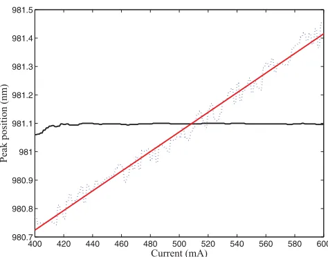
To test the prediction of Eq.(3), the same experiment has been done with a second telescope arrangement, i.e., a long cavity withf2=125 mm (M≈15) and Fig.9illustrates the shift in frequency of the VCSEL with this external cavity setup. The shift is barely noticeable, and within the accuracy range of our equipment it is not possible to quantify it. From Eq.(3) one expects to haveλ=λg−0.02 nm withM=15.6. This result is in good agreement with our experimental observation that the curve is essentially flat beyond the soliton region, i.e., above 430 mA. The remaining variations are below the limit of the accuracy of our optical spectral analyzer (about 0.03-nm relative accuracy within a single run). These results confirm the presence of frequency locking when feedback is provided from a VBG and also that the remaining frequency shift depends on the magnification factor of the external cavity. For a large magnification (M1),ba, one findsλ≈λg, i.e., perfect locking, because the dispersion relation of the VBG approaches a vertical line.
As derived in the previous section, the wavenumber of the emission should follow a square root behavior with detuning. Based on data like the ones obtained in Fig. 5 this can be checked quantitatively and the results are shown in Fig.10(a), which shows indeed a nice square-root behavior with a scaling
400 420 440 460 480 500 520 540 560 580 600
980.7 980.8 980.9 981 981.1 981.2 981.3 981.4 981.5
Current (mA)
Peak position (nm)
FIG. 9. (Color online) Solid black line: frequency shift of the VCSEL with feedback from a VBG (M=15.6). Dashed blue (light gray) line: FRL at 16◦C. Solid red (gray) line: fit to the FRL.
exponent of 0.502 with a negligible parameter error (on the order of 3×10⁻³) and a high-fidelity regression coefficient (R2 =0.9989) returned by the nonlinear fitting code.
V. EFFECTS OF DEVIATION FROM SELF-IMAGING
By these investigations, the effect of the VBG on wave-length locking is quite clear but the influence of the distances between the intra-cavity lenses (e.g.D2orD3) remains to be investigated. For example, Figs.3and5clearly indicate that D3has an influence on the spatial structures.
As shown in Fig.1, a self-imaging cavity is characterized by three distances. The first one is the distanceD1 between the laser and the collimation lens. It is found by adjusting the position of the lens until the divergence of the beam is minimal. The second distance,D2, is the distance separating both lenses, also referred to as the intracavity distance in the following; ideally it is (f1+f2). The last distance isD3, which separates the second lens and the VBG. It is determined by moving the VBG until the near-field image of the VCSEL has the sharpest boundaries. As indicated, matrix theory indicates that D2does not influence the imaging condition for the intensity distribution. SinceD2 is hence the most poorly defined one (in the sense that there is no obvious alignment criterion based on the VCSEL images as forD1 andD3, but only an estimated distance from the specifications of the lenses and the collimation experiment as explained in Sec.III A), we first turn our attention to it.
[image:5.608.63.285.69.170.2] [image:5.608.316.553.70.256.2]0 0.1 0.2 0.3 0.4 0.5 0.6 0.7 0.8 0
0.1 0.2 0.3 0.4 0.5 0.6 0.7
(a)
Detuning (nm)
Wave number (1/
µ
m)
0 0.1 0.2 0.3 0.4 0.5 0.6 0.7 0.8
0 0.1 0.2 0.3 0.4 0.5 0.6 0.7
Detuning (nm)
Wave number (1/
µ
m)
(b)
FIG. 10. (Color online) Transverse wave number of the emission versus detuning between emission wavelength and longitudinal resonance (crosses represent data points; solid lines, fits). These plots are produced from plots of the wave numberqvs the currentI by finding the intersectI0 and the scaling exponents using a fitting function,q(I)=c(I−I0)s. The interceptI0 then corresponds to the zero detuning condition. Starting from that, the rate of 0.0035 nm/mA is applied as a coefficient to define the detuning scaling, which is used to plot the fitting (red) curve. (a) ForD2=70.5 mm, leading to a scaling exponents=0.502; (b) forD2=78 mm, leading to a scaling exponents=0.479.
D2 =70.5 mm. For example, for D2=74 mm, the scaling exponent is 0.508 andR2=0.9874.
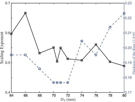
We also note that there is an enhanced tendency toward slight variations in the details of the patterns (not the basic structure) from run to run away fromD2=70.5 mm. Hence we report results averaged over three runs in Table I, which summarizes the effect of the intracavity distance on the scaling exponent over a larger range. Figure 11illustrates the same results graphically. The first observation is that, in general, the averaged scaling exponent oscillates around 0.5, with a tendency to larger values for smaller distances, but that there are actually two positions, atD2=74 and 78 mm, in addition toD2=70.5 mm at which the averaged scaling exponent is again close to 0.5. However, as stated above, the quality of the fits is lower and there is a larger variation between runs, which we characterize by the standard deviation σ of the scaling exponents returned for the different runs (TableI, last row).
In order to gain further insight into the nature of these deviations and variations, we analyzed the width of the ring in Fourier space as a measure of the quality of wave-number selection (Table I, second row, and Fig.11, dashed line). It has a minimum around D2=70.5 mm, i.e., the anticipated self-imaging condition, and increases, except for one exception interpreted as scatter, monotonically away from it. In particular, at 70.5 mm the ring is narrower than at
both 74 and 78 mm (see also the width in Table I). These observations reinforce our expectation thatD2=70.5 mm is the self-imaging position.
This behavior can be understood by the ABCD matrix for the round-trip through the external cavity ifD2=f1+f2+x, which reads
M2=
1 0
−2 f2
1
x 1
. (4)
A small mistuningx leads to a change in phase curvature or ray angle for the returning light. Hence the spatial Fourier spectrum broadens. Thus we conclude that D2=70.5 mm corresponds to the self-imaging distance. On a quantitative level, for a ray emerging at a distancerfrom the optical axis, the change in angle is
= − 2
f12 x r. (5)
[image:6.608.58.553.71.263.2]Taking r≈0.05 mm (half the radius of the VCSEL, i.e., an “average” r), and x =8 mm (the maximal deviation investigated in Fig. 11), one obtains =1.3×10⁻² and a corresponding change in wave number ofq =0.08μm−1. This is somewhat larger than, but comparable to, the maximum change in wave number observed in Fig. 11. A change
TABLE I. Effect ofD2on the scaling exponent. Three rounds of data-taking averaged. Data for both 70.5 and 72 mm are actually based on nine runs. The width of the ring in the far field is given as 500 mA.
DistanceD2
64 mm 66 mm 68 mm 70 mm 70.5 mm 71 mm 72 mm 74 mm 76 mm 78 mm 80 mm Scaling exponent 0.597 0.667 0.532 0.551 0.504 0.550 0.513 0.508 0.561 0.503 0.489 Width (1/μm) 0.195 0.195 0.186 0.176 0.176 0.176 0.176 0.204 0.195 0.214 0.223
Intersect (mA) 389 381 395 392 395 393 396 391 384 394 397
[image:6.608.49.558.666.752.2]64 66 68 70 72 74 76 78 80 0.4
0.5
0.6
0.7
Scaling Exponent
64 66 68 70 72 74 76 78 800.17
0.18 0.19 0.20 0.21 0.22 0.23
Thickness of the Rin
g
(
1/
µm)
D2 (mm)
FIG. 11. (Color online) Solid (black) line: scaling exponent vs.
D2. Dashed (blue) line: thickness of the ring in the far field vsD2.
of x =0.2 mm, the uncertainty in placing the lenses (see Sec. III A for details), yields only =3.1×10⁻⁴ and a corresponding change in wave number ofq =0.002μm−1, supporting the notion that there is some tolerance in placing the lenses.
Finally, we discuss the influence of D3 on the pattern formation. Figure 12 indicates that it also has an influence on the scaling exponent as well as on the manifestation of structures. We noted in Fig. 3 that for a cavity that is too long the near field seems to be pushed to the perimeter, whereas for a short cavity it seems to contract inward. The boundaries are not as sharp and well defined. Again, these features can be understood by ABCD-matrix theory, which gives, forD3=f2+x, a round-trip matrix of
M2=
1 2f12
f2 2
x
0 1
; (6)
i.e., the system is not imaging any more. For a ray emitted at a radiusrat an angle, the returning rays hit at
r=r+2f
2 1
f2
2
x. (7)
This means that for x >0 (cavity too long), the emission is pushed outward, whereas for x <0 (cavity too short) it is pushed inward. This is the tendency observed in the experiment. The effect should increase with increasing ray angle or wave number of emission, i.e., increasing current in our case, which seems to be supported by the evolution of images in Fig.3.
We investigated in Figs.3,5, and12a maximum variation ofx = ±4 mm; the highest transverse wave number in Fig.10 is smaller than 0.7μm−1. Then the (single-pass) shift from
Eq.(7)isr <20μm. For an uncertainty ofx=0.1 mm, it
is less than 1μm. Therefore one can expect thatD3 can be adjusted to an accuracy such that a potentially remaining devia-tion from the self-imaging condidevia-tion has a negligible influence on the pattern formation, especially in view of the fact that there is an explicit alignment criterion (sharpness of the images, e.g., Fig.3). From Eqs.(6)and(7)it is clear that the influence ofx
−4 −3 −2 −1 0 1 2 3 4
0.44 0.46 0.48 0.5 0.52 0.54 0.56 0.58 0.6 0.62 0.64
Position of the VBG (mm)
[image:7.608.53.291.70.249.2]Scaling exponent
FIG. 12. Scaling exponent as function ofD3. The zero position indicates the self-imaging position and a negative sign means that the VBG is moved toward the telescope. Inversely, a positive sign means that the VBG is moved away from the focusing lens.
onD3evolves asf12/f22, leaving the variation very small for f2f1. This is in line with the expectation from geometrical optics that the depth of focus at the VBG increases for large f2/f1 because the incidence angles decrease. Hence, a long cavity is beneficial for reducing the sensitivity to a misadjustment of D3 and for minimizing wavelength shifts (as discussed in Sec.IV) but comes at the expense of a large footprint and vibration sensitivity.
VI. CONCLUSION
We have established that VBGs work as wavelength lockers for VCSELs as well as for EELs, for which they are of significant importance for wavelength and modal control. VCSELs already have a lower temperature dependence than EELs because their wavelength shift is determined by a cavity shift of about 0.1 nm/K (for GaAs-based devices), compared to a gain shift of 0.2–0.3 nm/K relevant to EELs. Nevertheless, an external VBG can decrease this shift even more and the fidelity increases with increasing magnification of the imaging system, unfortunately increasing the footprint of the system.
[image:7.608.313.554.71.261.2]the mixture of low-order and high-order modes typical for broad-area EELs, but the average mode order will not increase as much as in the VCSEL.
We have also analyzed the effect of deviations of the external cavity from the self-imaging condition. It turns out that the system is remarkably insensitive to deviations even in the millimeter range for a cavity length in the 100-mm range. This is good news for the robustness of the experimental conditions. We remark that we consider the self-imaging condition to be attractive for these kind of experiments because it allows for the best feedback efficiency in terms of amplitude and phase. Not only does an autocollimation setup using only the collimation lens (as in Refs. [4,5]) introduce an image inversion (relevant for Gauss-Hermite modes, e.g.), but also, due to the shortness of the focal lengths of typical collimation lenses, it is likely that the length of the external cavity is larger than the perfect telescope length (an imperfectD2in our
terminology). Hence, there is a phase curvature of the returning beam for Gaussian modes and a chance of ray direction for Fourier modes and, as a result, an imperfect interference with the cavity mode. Deviations from the self-imaging conditions also make it more difficult to model the returning field distribution, though, in principle, methods like the Collins integral are available, of course [19]. On the other hand, a controlled deviation from the self-imaging condition might provide a convenient handle on coupling strength in arrays of lasers and laser solitons [10,12].
ACKNOWLEDGMENTS
Y.N. was supported by an EPSRC DTG. We are grateful to W. J. Firth and Jesus Jimenez-Garcia for useful discussions and to R. Jaeger (Ulm Photonics) for supplying the devices.
[1] B. L. Volodin, S. V. Dolgy, E. D. Melnik, E. Downs, J. Shaw, and V. S. Ban,Opt. Lett.29, 1891 (2004).
[2] M. Maiwald, A. Ginolas, A. M¨uller, A. Sahm, B. Sumpf, G. Erbert, and G. Tr¨ankle,IEEE Photon. Technol. Lett.20, 1627 (2008).
[3] F. Kroeger, I. Breunig, and K. Buse,Appl. Phys. B 95, 603 (2009).
[4] F. Marino, S. Barland, and S. Balle,IEEE Photon. Technol. Lett. 15, 789 (2003).
[5] Y. K. Chembo, S. K. Mandre, I. Fischer, W. Els¨aßer, and P. Colet, Phys. Rev. A79, 013817 (2009).
[6] M. Schulz-Ruhtenberg, Y. Tanguy, K. F. Huang, R. J¨ager, and T. Ackemann,J. Phys. D42, 055101 (2009).
[7] N. Radwell and T. Ackemann,IEEE J. Quantum Electron.45, 1388 (2009).
[8] T. Ackemann, G.-L. Oppo, and W. J. Firth,Adv. At. Mol. Opt. Phys.57, 323 (2009).
[9] P. V. Paulau, C. McIntyre, Y. Noblet, N. Radwell, W. J. Firth, P. Colet, T. Ackemann, and G.-L. Oppo, Phys. Rev. Lett. (in press, 2012).
[10] M. Nixon, M. Friedman, E. Ronen, A. A. Friesem, N. Davidson, and I. Kanter,Phys. Rev. Lett.106, 223901 (2011).
[11] M. Nixon, E. Ronen, A. A. Friesem, and N. Davidson, in The European Conference on Lasers and Electro-Optics (CLEO/Europe) and EQEC 2011 Conference Digest, OSA Tech-nical Digest (CD)(Optical Society of America, Massachusetts, Washington DC, USA, 2011), p. CA9_4.
[12] Y. Tanguy, T. Ackemann, W. J. Firth, and R. J¨ager,Phys. Rev. Lett.100, 013907 (2008).
[13] M. Grabherr, R. J¨ager, M. Miller, C. Thalmaier, J. Herlein, and K. J. Ebeling,IEEE Photon. Technol. Lett.10, 1061 (1998). [14] M. Grabherr, M. Miller, R. J¨ager, R. Michalzik, U. Martin, H. J.
Unold, and K. J. Ebeling,IEEE J. Sel. Top. Quantum Electron. 5, 495 (1999).
[15] M. Schulz-Ruhtenberg, Y. Tanguy, R. J¨ager, and T. Ackemann, Appl. Phys. B97, 397 (2009).
[16] M. Schulz-Ruhtenberg, I. Babushkin, N. A. Loiko, T. Ackemann, and K. F. Huang,Appl. Phys. B81, 945 (2005). [17] A. Naumenko, N. A. Loiko, M. Sondermann, K. F. Jentsch, and
T. Ackemann,Opt. Commun.259, 823 (2006).
[18] T. Ackemann, N. Radwell, Y. Noblet, and R. J¨ager,Opt. Lett. 37, 1079 (2012).