Search for gravitational waves from galactic and extra-galactic binary neutron stars

Search for gravitational waves from galactic and extra-galactic binary neutron stars

S. Ballmer,13B. C. Barish,12C. Barker,14D. Barker,14M. Barnes,12,bB. Barr,35M. A. Barton,12K. Bayer,13 R. Beausoleil,26,cK. Belczynski,23R. Bennett,35,dS. J. Berukoff,1,eJ. Betzwieser,13B. Bhawal,12I. A. Bilenko,20

G. Billingsley,12E. Black,12K. Blackburn,12L. Blackburn,13B. Bland,14B. Bochner,13,fL. Bogue,12R. Bork,12 S. Bose,40P. R. Brady,39V. B. Braginsky,20J. E. Brau,37D. A. Brown,12A. Bullington,26A. Bunkowski,2,31 A. Buonanno,6,gR. Burgess,13D. Busby,12W. E. Butler,38R. L. Byer,26L. Cadonati,13G. Cagnoli,35J. B. Camp,21 C. A. Cantley,35L. Cardenas,12K. Carter,15M. M. Casey,35J. Castiglione,34A. Chandler,12J. Chapsky,12,bP. Charlton,12,h

S. Chatterji,13S. Chelkowski,2,31Y. Chen,6V. Chickarmane,16,iD. Chin,36N. Christensen,8D. Churches,7 T. Cokelaer,7C. Colacino,33R. Coldwell,34M. Coles,15,jD. Cook,14T. Corbitt,13D. Coyne,12J. D. E. Creighton,39 T. D. Creighton,12D. R. M. Crooks,35P. Csatorday,13B. J. Cusack,3C. Cutler,1E. D’Ambrosio,12K. Danzmann,2,31

E. Daw,16,kD. DeBra,26T. Delker,1,34V. Dergachev,36R. DeSalvo,12S. Dhurandhar,11A. Di Credico,27 M. Dı´az,29H. Ding,12R. W. P. Drever,4R. J. Dupuis,35J. A. Edlund,12,bP. Ehrens,12E. J. Elliffe,35T. Etzel,12

M. Evans,12T. Evans,15S. Fairhurst,39C. Fallnich,31D. Farnham,12M. M. Fejer,26T. Findley,25M. Fine,12 L. S. Finn,28K. Y. Franzen,34A. Freise,2,mR. Frey,37P. Fritschel,13V. V. Frolov,15M. Fyffe,15K. S. Ganezer,5

J. Garofoli,14J. A. Giaime,16A. Gillespie,12,nK. Goda,13G. Gonza´lez,16S. Goßler,31P. Grandcle´ment,23,o A. Grant,35C. Gray,14A. M. Gretarsson,15D. Grimmett,12H. Grote,2S. Grunewald,1M. Guenther,14 E. Gustafson,26,pR. Gustafson,36W. O. Hamilton,16M. Hammond,15J. Hanson,15C. Hardham,26J. Harms,19

G. Harry,13A. Hartunian,12J. Heefner,12Y. Hefetz,13G. Heinzel,2I. S. Heng,31M. Hennessy,26N. Hepler,28 A. Heptonstall,35M. Heurs,31M. Hewitson,2S. Hild,2N. Hindman,14P. Hoang,12J. Hough,35M. Hrynevych,12,q

W. Hua,26M. Ito,37Y. Itoh,1A. Ivanov,12O. Jennrich,35,rB. Johnson,14W. W. Johnson,16W. R. Johnston,29 D. I. Jones,28L. Jones,28D. Jungwirth,12,sV. Kalogera,23E. Katsavounidis,13K. Kawabe,14S. Kawamura,22 W. Kells,12J. Kern,15,tA. Khan,15S. Killbourn,35C. J. Killow,35C. Kim,23C. King,12P. King,12S. Klimenko,34

S. Koranda,39K. Ko¨tter,31J. Kovalik,15,bD. Kozak,12B. Krishnan,1M. Landry,14J. Langdale,15B. Lantz,26 R. Lawrence,13A. Lazzarini,12M. Lei,12I. Leonor,37K. Libbrecht,12A. Libson,8P. Lindquist,12S. Liu,12 J. Logan,12,uM. Lormand,15M. Lubinski,14H. Lu¨ck,2,31T. T. Lyons,12,uB. Machenschalk,1M. MacInnis,13 M. Mageswaran,12K. Mailand,12W. Majid,12,bM. Malec,2,31F. Mann,12A. Marin,13,vS. Ma´rka,12,wE. Maros,12

J. Mason,12,xK. Mason,13O. Matherny,14L. Matone,14N. Mavalvala,13R. McCarthy,14D. E. McClelland,3 M. McHugh,18J. W. C. McNabb,28G. Mendell,14R. A. Mercer,33S. Meshkov,12E. Messaritaki,39C. Messenger,33 V. P. Mitrofanov,20G. Mitselmakher,34R. Mittleman,13O. Miyakawa,12S. Miyoki,12,yS. Mohanty,29G. Moreno,14

K. Mossavi,2G. Mueller,34S. Mukherjee,29P. Murray,35J. Myers,14S. Nagano,2T. Nash,12R. Nayak,11 G. Newton,35F. Nocera,12J. S. Noel,40P. Nutzman,23T. Olson,24B. O’Reilly,15D. J. Ottaway,13A. Ottewill,39,z

D. Ouimette,12,sH. Overmier,15B. J. Owen,28Y. Pan,6M. A. Papa,1V. Parameshwaraiah,14A. Parameswaran,1 C. Parameswariah,15M. Pedraza,12S. Penn,10M. Pitkin,35M. Plissi,35R. Prix,1V. Quetschke,34F. Raab,14

H. Radkins,14R. Rahkola,37M. Rakhmanov,34S. R. Rao,12K. Rawlins,13S. Ray-Majumder,39V. Re,33 D. Redding,12,bM. W. Regehr,12,bT. Regimbau,7S. Reid,35K. T. Reilly,12K. Reithmaier,12D. H. Reitze,34 S. Richman,13,aaR. Riesen,15K. Riles,36B. Rivera,14A. Rizzi,15,abD. I. Robertson,35N. A. Robertson,26,35 L. Robison,12S. Roddy,15J. Rollins,13J. D. Romano,7J. Romie,12H. Rong,34,nD. Rose,12E. Rotthoff,28 S. Rowan,35A. Ru¨diger,2P. Russell,12K. Ryan,14I. Salzman,12V. Sandberg,14G. H. Sanders,12,acV. Sannibale,12

B. Sathyaprakash,7P. R. Saulson,27R. Savage,14A. Sazonov,34R. Schilling,2K. Schlaufman,28V. Schmidt,12,ad R. Schnabel,19R. Schofield,37B. F. Schutz,1,7P. Schwinberg,14S. M. Scott,3S. E. Seader,40A. C. Searle,3

B. Sears,12S. Seel,12F. Seifert,19A. S. Sengupta,11C. A. Shapiro,28,aeP. Shawhan,12D. H. Shoemaker,13 Q. Z. Shu,34,afA. Sibley,15X. Siemens,39L. Sievers,12,bD. Sigg,14A. M. Sintes,1,32J. R. Smith,2M. Smith,13 M. R. Smith,12P. H. Sneddon,35R. Spero,12,bG. Stapfer,15D. Steussy,8K. A. Strain,35D. Strom,37A. Stuver,38

T. Summerscales,28M. C. Sumner,12P. J. Sutton,12J. Sylvestre,12,agA. Takamori,12D. B. Tanner,34H. Tariq,12 I. Taylor,7R. Taylor,35R. Taylor,12K. A. Thorne,28K. S. Thorne,6M. Tibbits,28S. Tilav,12,ahM. Tinto,4,b

A. Weinstein,12R. Weiss,13H. Welling,31L. Wen,12S. Wen,16J. T. Whelan,18S. E. Whitcomb,12B. F. Whiting,34 S. Wiley,5C. Wilkinson,14P. A. Willems,12P. R. Williams,1,ajR. Williams,4B. Willke,31A. Wilson,12 B. J. Winjum,28,eW. Winkler,2S. Wise,34A. G. Wiseman,39G. Woan,35D. Woods,1R. Wooley,15J. Worden,14 W. Wu,34I. Yakushin,15H. Yamamoto,12S. Yoshida,25K. D. Zaleski,28M. Zanolin,13I. Zawischa,31,akL. Zhang,11

R. Zhu,1N. Zotov,17M. Zucker,15and J. Zweizig12

(LIGO Scientific Collaboration)

1_{Albert-Einstein-Institut, Max-Planck-Institut fu¨r Gravitationsphysik, D-14476 Golm, Germany} 2

Albert-Einstein-Institut, Max-Planck-Institut fu¨r Gravitationsphysik, D-30167 Hannover, Germany 3_{Australian National University, Canberra, 0200, Australia}

4_{California Institute of Technology, Pasadena, California 91125, USA} 5_{California State University Dominguez Hills, Carson, California 90747, USA}

6_{Caltech-CaRT, Pasadena, California 91125, USA} 7_{Cardiff University, Cardiff, CF2 3YB, United Kingdom}

8_{Carleton College, Northfield, Minnesota 55057, USA} 9_{Fermi National Accelerator Laboratory, Batavia, Illinois 60510, USA} 10_{Hobart and William Smith Colleges, Geneva, New York 14456, USA} 11_{Inter-University Centre for Astronomy and Astrophysics, Pune-411007, India} 12_{LIGO—California Institute of Technology, Pasadena, California 91125, USA} 13_{LIGO—Massachusetts Institute of Technology, Cambridge, Massachusetts 02139, USA}

14_{LIGO Hanford Observatory, Richland, Washington 99352, USA} 15_{LIGO Livingston Observatory, Livingston, Louisiana 70754, USA}

16_{Louisiana State University, Baton Rouge, Louisiana 70803, USA} 17_{Louisiana Tech University, Ruston, Louisiana 71272, USA}

18_{Loyola University, New Orleans, Louisiana 70118, USA} 19_{Max Planck Institut fu¨r Quantenoptik, D-85748, Garching, Germany}

20_{Moscow State University, Moscow, 119992, Russia}

21_{NASA/Goddard Space Flight Center, Greenbelt, Maryland 20771, USA} 22_{National Astronomical Observatory of Japan, Tokyo 181-8588, Japan}

23_{Northwestern University, Evanston, Illinois 60208, USA} 24_{Salish Kootenai College, Pablo, Montana 59855, USA} 25_{Southeastern Louisiana University, Hammond, Louisiana 70402, USA}

26_{Stanford University, Stanford, California 94305, USA} 27_{Syracuse University, Syracuse, New York 13244, USA}

28_{The Pennsylvania State University, University Park, Pennsylvania 16802, USA}

29_{The University of Texas at Brownsville and Texas Southmost College, Brownsville, Texas 78520, USA} 30_{Trinity University, San Antonio, Texas 78212, USA}

31_{Universita¨t Hannover, D-30167 Hannover, Germany} 32_{Universitat de les Illes Balears, E-07122 Palma de Mallorca, Spain}

33_{University of Birmingham, Birmingham, B15 2TT, United Kingdom} 34_{University of Florida, Gainesville, Florida 32611, USA} 35_{University of Glasgow, Glasgow, G12 8QQ, United Kingdom}

36_{University of Michigan, Ann Arbor, Michigan 48109, USA} 37_{University of Oregon, Eugene, Oregon 97403, USA} 38_{University of Rochester, Rochester, New York 14627, USA} 39_{University of Wisconsin –Milwaukee, Milwaukee, Wisconsin 53201, USA}

40_{Washington State University, Pullman, Washington 99164, USA}

(Received 30 May 2005; published 25 October 2005)

galaxy with 90% confidence for nonspinning binary neutron star systems with component masses between 1 and3M.

DOI:10.1103/PhysRevD.72.082001 PACS numbers: 95.85.Sz, 04.80.Nn, 07.05.Kf, 97.80.2d

I. INTRODUCTION

The search for gravitational waves has entered a new era with the scientific operation of kilometer scale laser inter-ferometers. These L-shaped instruments are sensitive to minute changes in the relative lengths of their orthogonal arms that would be produced by gravitational waves [1]. The Laser Interferometer Gravitational-wave Observatory (LIGO) [2,3] consists of three Fabry-Perot-Michelson in-terferometers: two interferometers are housed at the site in Hanford, WA; a single interferometer is housed in Livingston, Louisiana. In 2003, all three instruments si-multaneously collected data under stable operating condi-tions during two science runs. Even though the instruments

were not yet performing at their design sensitivity, the data represent the best broadband sensitivity to gravitational waves that has been achieved to date.

In this paper, we report the methods and results of a search for gravitational waves from binary neutron star systems, using data from the science run conducted early in 2003. These waves are expected to be emitted at fre-quencies detectable by LIGO during the final few seconds of inspiral as the binary orbit decays due to the loss of energy in gravitational radiation [4]. A previous search [5], using data from the first LIGO science run, reported an upper limit on the rate of coalescences within our Galaxy and the magellanic clouds. This paper uses an analysis pipeline which is optimized for detection by using data only from times when interferometers were operating properly at both LIGO sites. By demanding that a gravita-tional wave be seen at both sites, we strongly suppress the rate of background events from nonastrophysical distur-bances. Moreover, this approach allows us to judge the significance of any apparent event candidate in the context of the background distribution, which is also determined from the data.

The search described here has essentially perfect effi-ciency for detecting binary neutron star inspirals within the Milky Way and the magellanic clouds (as measured by Monte-Carlo simulations), and could detect some inspirals as far away as the Andromeda and Triangulum galaxies (M31 and M33). The rate of coalescences in these galaxies, based on the population of known binary neutron star systems [6], is expected to be very low, so that a detection by the present search would be highly surprising. In fact, no coincident event candidates were observed in excess of the measured background. The data are therefore used to place an improved direct observational upper limit on the rate of binary neutron star coalescence events in the Universe.

II. DATA SAMPLE

The LIGO Hanford Observatory (LHO) in Washington state has two independent detectors sharing a common vacuum envelope, one with 4 km long arms (H1) and one with 2 km long arms (H2). The LIGO Livingston Observatory (LLO) in Louisiana has one detector with 4 km long arms (L1). All three detectors operated during the second LIGO science run, referred to as S2, which spanned 59 days from February 14 to April 14, 2003. During operation, feedback to the mirror positions and to the laser frequency keeps the optical cavities near reso-nance, so that interference in the light from the two arms recombining at the beam splitter is strongly dependent on a_{Currently at Stanford Linear Accelerator Center.}

b_{Currently at Jet Propulsion Laboratory.}

ah_{Currently at University of DE.}

ak_{Currently at Laser Zentrum Hannover.}

ai_{Permanent Address: Jet Propulsion Laboratory.} ag_{Permanent Address: IBM Canada Ltd.}

ae_{Currently at University of Chicago.}

aj_{Currently at Shanghai Astronomical Observatory.}

ad_{Currently at European Commission, DG Research, Brussels,}

Belgium.

ac_{Currently at Thirty Meter Telescope Project at Caltech.} ab_{Currently at Institute of Advanced Physics, Baton Rouge, LA.}

z_{Permanent Address: University College Dublin.}

af_{Currently at LightBit Corporation.}

t_{Currently at NM Institute of Mining and Technology/}

Magdalena Ridge Observatory Interferometer.

w_{Permanent Address: Columbia University.}

aa_{Currently at Research Electro-Optics Inc.} v_{Currently at Harvard University.}

s

Currently at Raytheon Corporation.

x_{Currently at Lockheed-Martin Corporation.}

y_{Permanent Address: University of Tokyo, Institute for}

Cosmic Ray Research.

r_{Currently at ESA Science and Technology Center.}

u_{Currently at Mission Research Corporation.} q_{Currently at W. M. Keck Observatory.} p_{Currently at Lightconnect Inc.}

o_{Currently at University of Tours, France.} n_{Currently at Intel Corp.}

m_{Currently at European Gravitational Observatory.} l_{Currently at Ball Aerospace Corporation.} i_{Currently at Keck Graduate Institute.} j_{Currently at National Science Foundation.}

g_{Permanent Address: GReCO, Institut d’Astrophysique de}

Paris (CNRS).

k_{Currently at University of Sheffield.} e_{Currently at University of CA, Los Angeles.}

h_{Currently at La Trobe University, Bundoora VIC, Australia.} c_{Permanent Address: HP Laboratories.}

f_{Currently at Hofstra University.}

the difference between the lengths of the two arms. A photodiode at the antisymmetric port of the detector senses this light, and a digitized signal is recorded at a sampling rate of 16 384 Hz. This channel can then be searched for a gravitational-wave signal. More details on the detectors’ instrumental configuration and performance can be found in [3,7].

While the detailed noise spectrum of a detector affects different gravitational-wave searches in different ways, we can summarize the sensitivity of a detector for low-mass inspiral signals in terms of the range for an archetypal source. Specifically, the range is the distance at which an optimally oriented and located binary system1 with the mass of each component equal to1:4M would yield an

amplitude signal-to-noise ratio (SNR) of 8 when extracted from the data using optimal filtering. During the first LIGO science run (referred to as S1), the L1 detector had the greatest range, typically 0.18 Mpc. During the S2 run, all three detectors were substantially more sensitive than this, with ranges of 2.0, 0.9, and 0.6 Mpc for L1, H1, and H2 averaged over all times during the run. Typical amplitude spectral densities of detector noise are shown in Fig. 1.

The amount of science data with good performance and stable operating conditions was limited by environmental factors (especially high ground motion at LLO and strong winds at LHO), occasional equipment failures, and peri-odic special investigations. Over the 1415 h duration of the S2 run, the total amount of science data obtained was 536 hours for L1, 1044 hours for H1, and 822 hours for H2.

The analysis presented here uses data collected while the LLO detector was operating at the same time as one or both of the LHO detectors. Science data during which both H1 and H2 were operating but L1 was not, amounting to 385 hours, was not used in this analysis because of concerns about possible environmentally induced correlations be-tween the data streams of these two colocated detectors; this data set, as well as data collected while only one of the LIGO detectors was in science mode, will be used in a separate analysis together with data from the TAMA300 detector [8], which conducted ‘‘Data Taking 8’’ concur-rently with the LIGO S2 run.

Of all the data, approximately 9% (uniformly sampled within the run so as to be representative of the whole data set) was used asplaygrounddata for tuning parameters and thresholds in the analysis pipeline, and for use in identify-ing vetoes that were effective in eliminatidentify-ing spurious events. This playground data set was excluded from the gravitational-wave inspiral upper limit calculation because event selection and pipeline tuning, as described in Secs. IV, V, and VI, introduces statistical bias which cannot be accounted for. The playground data set was searched for

inspiral signals, however, so a potential detection during these times was not excluded. After applying data quality cuts (as detailed in Sec. V) and accounting for short time intervals which could not be searched for inspiral signals by the filtering algorithm (described in Sec. IV), the ob-servation time consisted of 242 hours of triple-detector data, plus 99 hours of L1-H1 and 32 hours of L1-H2 data, for a total observation time of 373 hours. For the upper limit result, the nonplayground observation time was 339 hours. A summary of the amount of single-, double-, and triple-detector times is provided in Fig. 2.

102 103

10−23 10−22 10−21 10−20 10−19 10−18

frequency(Hertz)

strain/

√⎯⎯

⎯

Hz

S1: L1 (9 Sept ’02) S2: L1 (1 March ’03) S2: H1 (8 April ’03) S2: H2 (11 April ’03)

FIG. 1 (color online). Typical sensitivities, expressed as am-plitude spectral densities of detector noise converted to equiva-lent gravitational-wave strain, for the best detector during the S1 run (the Livingston detector) and for all three detectors during the S2 run. The solid lower line is the design sensitivity for the LIGO 4-km detectors; the dashed line is the design sensitivity for the LIGO 2-km detector at Hanford.

FIG. 2. The number of hours that each detector combination was operational during the S2 run. The upper number gives the amount of time the specific instruments were coincidentally operational. The lower number gives the total time that was searched for inspiral triggers. The shaded region corresponds to the data used in this search.

1_{An optimally oriented and located binary system would be}

As with earlier analyses of LIGO data [5], the output of the antisymmetric port of the detector was calibrated to obtain a measure of the relative strain sL=L of the detector arms, where LL_xL_y is the difference in length between one arm (the xarm) and the other (the y

arm), and L is the average arm length.

Reference calibration functions, tracing out the frequency-dependent response of the detectors, were mea-sured (by moving the end mirrors of the detector with a known displacement) before and after the science run, and once during the science run; all three measurements gave consistent results. The changing optical gain of the cali-bration was monitored continuously during the run by applying sinusoidal motions with fixed frequency to the end mirrors. This continuous monitoring, averaged once a minute, allowed for small corrections to the calibration due to loss of light power in the arms, which can be caused by drifting optical alignment.

III. TARGET SOURCES

Binary neutron star (BNS) systems in the Milky Way, known from radio pulsar observations [9], provide indirect evidence for the existence of gravitational waves [10]. Based on current astrophysical understanding, the spatial distribution of binary neutron stars is expected to follow that of star formation in the Universe. A measure of star formation is the blue luminosity of galaxies appropriately corrected for dust extinction and reddening. Therefore we model the spatial distribution of double neutron stars ac-cording to the corrected blue-light distribution of nearby galaxies [11]. While the masses of neutron stars in the few known binary systems are all near1:4M, population

syn-thesis simulations suggest that some systems will have component masses as low as 1M and as high as the

theoretical maximum neutron star mass of 3M [12].

Thus, we search for inspiral signals from binary systems with component masses in this range. Note that the higher-mass systems radiate more energy in gravitational waves and can thus be detected at a greater distance at a given SNR. For component masses below 1M, a search is

reported in Ref. [13].

When the LIGO detectors reach their design sensitiv-ities, they will be capable of detecting inspiral signals from thousands of galaxies, reaching beyond the Virgo Cluster for systems with optimal location and orientation. At that sensitivity, the rate of detectable binary neutron star co-alescences could be as high as 0.7 per year, though it is more likely to be an order of magnitude smaller [6]. For this analysis, our target population includes the Milky Way and all significant galaxies within a distance of 3 Mpc, which is roughly the maximum distance for which a

3–3M inspiral could be detected in coincidence by the

L1 and H1 interferometers with a SNR of 6 in H1. This population includes the Local Group of galaxies, whose total blue luminosity is dominated by the Andromeda

Galaxy (M31), as well as some galaxies from neighboring groups. We cannot hope to detectallinspirals within this volume, because most systems in the population have lower masses and because the received signal amplitude is reduced, on average, depending on the orientation and location of the source relative to the detector.

Table I gives the parameters we use for the galaxies in the target population out to 1.5 Mpc, i.e., the maximum distance for which we had a nonzero detection efficiency in our simulations. The coordinates and distances of the galaxies in Table I are taken from a catalog by Mateo [14], when available; this catalog is favored because dis-tances quoted are from individual, focused studies of each of the nearby galaxies he includes. The rest of the dis-tances, with only 100 kpc accuracy, are taken from the Tully Nearby Galaxies catalog [15]. Data for blue lumi-nosities are derived from the apparent blue magnitudes (corrected for reddening) quoted in Ref. [16], and the distances shown in Table I. We measured the efficiency of our search using Monte-Carlo simulations, where the sources in the target population had a mass distribution as described in Ref. [12], following the same guidelines as in the population models used in Ref. [17]. We used simula-tions with a population of neutron stars from galaxies up to 3 Mpc away, overextending our target population, although we did not detect any simulated injections from sources farther than 1.5 Mpc away.

Within the LIGO frequency band, the gravitational waveform produced by binary neutron star systems is well described by the restricted second-post-Newtonian approximation [18–20]. The spins of the neutron stars are not expected to significantly affect the orbital motion or the waveform [18]. Tidal coupling and other finite-body effects dependent on the equation of state also are not expected to significantly affect the waveform in the LIGO band [21]. The waveform received at Earth is there-fore parametrized by the masses of the companions, the distance to the binary, the inclination of the system to the plane of the sky, and by the initial orbital phase when the waveform enters the LIGO band. The waveforms consist of two polarizations, the plus (h) and cross (h)

polariza-tions, which describe the two orthogonal tidal distortions produced by the waves. These polarization basis states are defined with respect to the orientation of the binary orbit relative to the line of sight. An interferometric detector is sensitive to a particular linear combination of these two polarizations; this is described by two response functions

FandFso that the expected gravitational-wave signal

is

ht Fht Fht : (1)

aligned as closely as possible, but the curvature of the Earth causes a slight difference in their antenna patterns.

IV. FILTERING AND TRIGGER GENERATION

We generated event triggers by filtering the data st

from each detector with matched filters designed to detect the expected signals. For any given binary neutron star mass pair, fm₁; m₂g, we constructed the expected frequency-domain inspiral waveform template,h~f , using a stationary-phase approximation to the restricted second-post-Newtonian waveform [22].2Here, the tilde indicates the Fourier transform of a time seriesht according to the convention

~

hf Z1 1

hte2ift_{dt: (2)}

The matched filter output is then the complex time series

zt xt iyt 4Z1 0

~

hf ~sf Sf e

2ift_{df (3)}

wherext is the (real) matched filter output for the inspiral waveform with a zero orbital phase, andyt is the (real) matched filter output for the inspiral waveform with a=2

orbital phase. The quantity Sf is the one-sided strain noise power spectral density, estimated from the data. The matched filter variance is given by

2 ₄Z1 0

j_h~_{f j}2

Sf df (4)

which depends on the template’s amplitude normalization. The amplitude SNR is then

jzj=: (5)

The templates were normalized to a binary neutron star inspiral at aneffective distanceof 1 Mpc, where the effec-tive distance of a waveform is the distance for which a binary neutron star system would produce the waveform if it were optimally oriented. Thus,

0.010 0.1 1 3 0.2

0.4 0.6 0.8 1

Effective Distance (Mpc)

NG

L1 H1 H2 S1

0.010 0.1 1 3 1

2 3 4

Effective Distance (Mpc)

Cumulative N

G

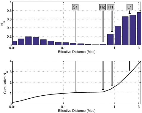
FIG. 3 (color online). The upper panel shows the histogram of the number of Milky Way equivalent galaxies (NG) as a function ofeffectivedistance. Labeled arrows indicate the average range of the best detector in the first science run (S1), as well as the average range of each detector during the second science run. The cumulative total within a given effective distance is shown in the bottom panel.

TABLE I. The galaxies in our population within 1.5 Mpc. The next to last column indicates the number of injections detected in coincidence (with signal-to-noise-ratio defined in Eq. (10) satisfying 2_{>89), over the number of injections performed in our}

simulations. The last column indicates the cumulative number of equivalent Milky Way galaxies contributed by systems within the corresponding distance, calculated from the search efficiency and the blue-light luminosity.

Name Right ascension

(Hour:Min)

Declination (Deg:Min)

Distance (kpc)

Blue-light luminosity relative to Milky Way

Detected/injected with2_>89

Cumulative

NG

Milky Way 1 686/686 1

LMC 05:23:6 69:45 49 0.128 57/57 1.128

SMC 00:52:7 72:50 58 0.037 8/8 1.165

NGC6822 19:44:9 14:49 490 0.01 0/4 1.165

NGC185 00:39:0 48:20 620 0.007 1/3 1.1673

M110 00:40:3 41:41 815 0.018 5/100 1.1682

M31 00:42:7 41:16 770 2.421 108/1791 1.3142

M32 00:42:7 40:52 805 0.019 9/129 1.3155

IC10 00:20:4 59:18 825 0.031 1/10 1.3186

M33 01:33:9 30:39 840 0.319 9/219 1.3318

NGC300 00:54:9 37:41 1200 0.052 1/40 1.3331

M81 09:55:6 69:04 1400 0.196 1/147 1.3344

NGC55 00:14:9 39:11 1480 0.175 2/122 1.3373

2_{The stationary-phase approximation to the Fourier transform}

D_eff

(6)

is an estimate of the effective distance, in Mpc, of a putative signal that produces SNR . The number of Milky Way equivalent galaxies as a function of effective distance is shown in Fig. 3.

Since each binary neutron star mass pairfm₁; m₂gwould produce a slightly different waveform, we constructed a bankof templates with different mass pairs such that, for any actual mass pair with 1Mm2m13M, the

loss of SNR due to the mismatch of the true waveform from that of the best fitting waveform in the bank is less than 3% [24,25].

Although a threshold on the matched filter output

would be the optimal detection criterion for an accurately known inspiral waveform in the case of stationary, Gaussian noise, the character of the data used in this analysis is known to be neither stationary nor Gaussian. Indeed, many classes of transient instrumental artifacts have been categorized, some of which produce copious numbers of spurious, large SNR events. In order to reduce the number of spurious event triggers, we adopted a now-standard2_{requirement [26]: The matched filter template}

is divided intopfrequency bands, which are chosen so that each band would contribute a fraction1=pof the total SNR if a true signal (and no detector noise) were present. In our analysis, we usedp15, as explained in Sec. VI B. We then construct a chi-squared statistic comparing the mag-nitude and phase of SNR accumulated in each band to the expected amount. For a true signal in Gaussian noise, the resulting statistic is2 _{distributed with2p2degrees of}

freedom (since the SNR is constructed out of the two matched filters x and y which are both measured). Instrumental artifacts tend to produce very large2values and can be rejected by requiring2 to be less than some reasonable threshold. Because of the discreteness of the template bank, however, a real signal will generally not match precisely the nearest template in the bank. Consequently,2_{has a noncentral chi-squared distribution}

with a noncentrality parameter p122_{, where}

is the fractional loss of SNR due to mismatch between template and signal [26]. For sufficiently small and moderate values of , this effect is not important, but when is large, it must be taken into account. This is done by applying a threshold with the following parame-trization:

2 _p22 _{: (7)}

The threshold multiplier, the number of binsp, and the value of were determined by tuning on the playground data, as will be described in Sec. VI B.

In this analysis, the SNRt was computed for each template in the bank [27]. Whenever t exceeded a threshold, the value of2 _{was computed for that time.}

If 2 was below the threshold in Eq. (7), then the local maximum oft was recorded as atrigger. Each trigger is

represented by a vector of values: the masses which define the template, the maximum value ofand corresponding value of 2_{, the inferred coalescence time, the effective}

distanceD_eff, and the coalescence phase ₀tan1_y=x.

V. DATA QUALITY CHECKS AND VETOES

In practice, the performance of the matched filtering algorithm described above is influenced by nonstationary optical alignment, servo control settings, and environmen-tal conditions. We used two strategies to avoid problematic data in this search. One was to evaluate data qualityover relatively long time intervals, using several different tests. Time intervals identified as being suspect or demonstrably bad were skipped when filtering the data. The other method was to look for signatures in environmental monitoring channels and auxiliary interferometer channels which would indicate an external disturbance or instrumental glitch (a large transient fluctuation), allowing us to veto any triggers recorded at that time.

Several data quality tests were applieda priori, leading us to omit data when calibration information was missing or unreliable, servo control settings were not at their nomi-nal values, or there were input/output controller timing problems. Additional tests were performed to characterize the noise level in the interferometer in various frequency bands and to check for problems with the photodiodes and associated electronics. The playground data set was used to judge the relevance of these additional tests, and two data quality tests were found to correlate with inspiral triggers found in the playground. One of these pertained only to the H1 interferometer; there were occasional, abnormally high noise levels in the H1 antisymmetric port channel that were apparent when this signal was averaged over a minute. Data was rejected only if this excessive noise was present for at least 3 consecutive minutes. The other data quality test used to reject data pertained to saturation of the pho-todiode at the antisymmetric port. These phopho-todiode satu-ration events correlated with a small, but significant, number of L1 inspiral triggers. We required the absence of photodiode saturation in the data from all three detectors.

coupling. This possibility was tested by means ofhardware injections, in which a simulated inspiral signal is injected into the data by physically moving one of the end mirrors of the interferometer. These hardware injections were used for validation of the analysis pipeline, as described in Sec. VI C. Unlike the software injections that are used to measure the pipeline efficiency (described in Sec. VI B), these hardware injections allow us to establish a limit on the effect that a true signal would have on the auxiliary channels. Only those channels that were unaffected by the hardware injections were considered safe for use as poten-tial veto channels.

We used an analysis program,glitchMon, [28] to iden-tify large amplitude transient signals in auxiliary channels. Numerous channels were examined by glitchMon, which generates a list of times when glitches occurred, identified by a filtered time series crossing a chosen threshold. A veto condition based on a given list of glitchMon triggers was defined by choosing a fixed time window around each glitch and rejecting any inspiral event trigger with a co-alescence time within the window.

For each veto condition considered, we evaluated the veto efficiency (percentage of inspiral events eliminated), use percentage (percentage of veto triggers which veto at least one inspiral event), and dead time (percentage of science-data time eliminated by the veto). Once a channel was identified, some tuning was done of the filters used, and the thresholds and time windows chosen, to optimize the efficiency, especially for high SNR candidates, without an excessive dead time. The parameter tuning was done only with the inspiral triggers found in the playground.

No efficient candidate veto channels were identified for H1 and H2; there were some candidates for L1. Nonstationary noise in the low-frequency part of the sen-sitivity range used for the inspiral search appeared to be the dominant cause for glitch events in the data. The original frequency range for the binary neutron star inspiral search extended from 50 Hz to 2048 Hz. It was discovered that many of the L1 inspiral triggers appeared to be the result of nonstationary noise with frequency content around 70 Hz. An important auxiliary channel, L1:LSC-POB_I, propor-tional to the length fluctuations of the power recycling cavity, was found to have highly variable noise at 70 Hz. As a consequence, it was decided that the low-frequency cutoff of the binary neutron star inspiral search should be increased from 50 Hz to 100 Hz. This subsequently re-duced the number of inspiral triggers. An inspection of artificial signals injected into the data revealed a very small loss of efficiency for binary neutron star inspiral signal detection resulting from the increase in the low-frequency cutoff.

Even after raising the low-frequency cutoff, the L1:LSC-POB_I channel was found to be an effective veto when filtered appropriately. Because of the characteristics of the inspiral templates’ response to large glitches, we decided to

veto with a very wide time window,4 sto8 s, around the time of each L1:LSC-POB_I trigger. With this choice, 12% of the BNS inspiral triggers with >8in the play-ground were vetoed, as well as 5 out of the 9 triggers found in the playground with >10. The use percentage of the veto triggers was 18% for >8 and 0.7% for >10, whereas values of 3% and<0:1%(respectively) would be expected from random coincidences if the veto triggers had no real correlation with the inspiral triggers. The total L1 dead time using this veto condition in the playground was 2.7%. The performance in the full data set was consistent with that found in the playground: the final observation time (including playground) was reduced by this veto from 385 hours to 373 hours. A more extensive discussion of LIGO’s S2 binary inspiral veto study can be found in [29].

VI. SEARCH FOR COINCIDENT EVENT CANDIDATES

A. Analysis pipeline

The detection of a gravitational-wave inspiral signal in the S2 data would (at the least) require triggers in L1 and one or more of the Hanford instruments with consistent arrival times (separated by the light travel time between the detectors) and waveform parameters. Requiring temporal coincidence between the two observatories greatly reduces the background rate due to spurious triggers, thus allowing an increased confidence for detection candidates. When detectors at both observatories are operating simulta-neously, we may obtain an estimate of the rate of back-ground triggers by time shifting the Hanford triggers with respect to the Livingston triggers and applying the same coincidence requirements to the time-shifted triggers, as described in Sec. VII. In this way, we can measure the rate of accidental coincidences in our search.

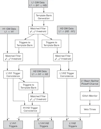
During the S2 run, the three LIGO detectors had sub-stantially different sensitivities. The sensitivity of the L1 detector was greater than that of either Hanford detector throughout the run. Since the orientations of the LIGO interferometers are similar, we expect that signals of as-trophysical origin detected in the Hanford interferometers generally are detectable in the L1 interferometer. Using this as a guiding principle, we have constructed a triggered search pipeline, summarized in Fig. 4. We search for inspiral triggers in the most sensitive interferometer (L1), and only when a trigger is found in this interferometer do we search for a coincident trigger in the less sensitive interferometers. This approach reduces significantly the computational power necessary to perform the search, without compromising the detection efficiency of the pipeline.

inter-ferometers were operating, and (3) times when only the L1 and H2 interferometers were operating. The pipeline pro-duces a list of coincident triggers for each of these three data sets as described below.

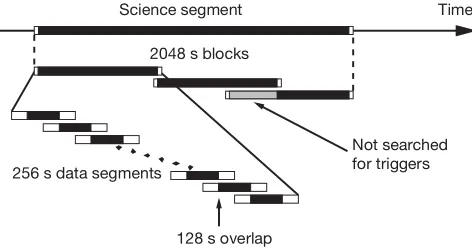
The science segments were analyzed in blocks of 2048 seconds using theFINDCHIRP implementation of matched filtering for inspiral signals in the LIGO Algorithm Library [30]. In this code, the data set for each 2048 s block is first down-sampled from 16 384 Hz to 4096 Hz. It is subse-quently high-pass filtered and a low-frequency cutoff of 100 Hz imposed. The calibrated instrumental response for the block is calculated using the average of the calibrations (measured every minute) over the duration of the block.

Triggers are not searched for within the first and last 64 s of a given block, so subsequent blocks are overlapped by 128 s to ensure that all of the data in a continuous science segment (except for the first and last 64 seconds) are searched for triggers. Any science segments shorter than 2048 s are ignored. If a science segment cannot be exactly divided into overlapping blocks (as is usually the case) the remainder of the data set is covered by a special 2048-s block which overlaps with the previous block as much as necessary to allow it to reach the end of the segment. For this final block, a parameter is set to restrict the inspiral search to the time interval not covered by any previous block, as shown in Fig. 5.

FIG. 4. The inspiral analysis pipeline used to determine the reported upper limit.L1\ H1[H2 indicates times when the L1 interferometer was operating in coincidence with one or both of the Hanford interferometers.L1\H1indicates times when the L1 interferometer was operating in coincidence with the H1 interferometer.L1\ H2H1 indicates times when the L1 interferometer was operating in coincidence with only the H2 interferometer. The outputs of the search pipeline are triggers that belong to one of the two double-detector coincident data sets or to the triple-detector data set.

Each block is further split into 15 data segments of length 256 seconds overlapped by 128 seconds. The power spectrumSf for the 2048 seconds of data is estimated by taking the median of the power spectra of the 15 segments. (We use the median and not the mean to avoid biased estimates due to large outliers, produced by nonstationary data.) The average calibration is applied to the data in each data segment, and the matched filter output in Eq. (3) is computed for each template in the template bank.

In order to avoid end effects when applying the matched filter, the frequency-weighting factor, nominally1=Sf, is altered so that its inverse Fourier transform has a maximum duration of16seconds. The output of the matched filter near the beginning and end of each segment is corrupted by end effects due to the finite duration of the power spectrum weighting and also the inspiral template. By ignoring the filter output within 64 s of the beginning and end of each segment, we ensure that only uncorrupted filter output is searched for inspiral triggers. This necessitates the over-lapping of segments and blocks as described above.

The power spectral density (PSD) of the noise in the Livingston detector is estimated independently for each L1 block that is coincident with operation of a Hanford detec-tor [denotedL1\ H1[H2]. The PSD is used to lay out a template bank for filtering that block, according to the parameters for mass ranges and minimal match [24,25]. The data from the L1 interferometer for the block are then filtered, using that bank, with a signal-to-noise threshold

_Land2_{veto threshold}

Lto produce a list of triggers as

described in Sec. IV. For each block in the Hanford

inter-ferometers, atriggered bankis created consisting of every template which produced at least one trigger in L1 during the time of the Hanford block. This is used to filter the data from the Hanford interferometers with signal-to-noise and

2 _{thresholds specific to the interferometer, giving a total}

of six thresholds that may be tuned. For times when only the H2 interferometer is operating in coincidence with L1 [denoted L1\ H2H1] the triggered bank is used to filter the H2 blocks that overlap with L1 data; these triggers are used to test for L1/H2 coincidence. All H1 data that overlaps with L1 data (denotedL1\H1) are filtered using the triggered bank for that block. For H1 triggers produced during times when all three interferometers were operat-ing, a second triggered bank is produced for each H2 block consisting of every template which produced at least one trigger found in coincidence in L1 and H1 during the time of the H2 block. The H2 block is filtered with this bank. Any H2 triggers found with this bank are tested for triple coincidence with the L1 and H1 triggers. The remaining triggers from H1, when H2 is not available, are used to search for L1/H1 coincident triggers.

For a trigger to be considered coincident between two interferometers, the following conditions must be fulfilled: (1) Triggers must be observed in both interferometers within a temporal coincidence window that allows for the error in measurement of the time of the trigger,t. If the detectors are not colocated, this parameter is increased by the light travel time between the observatories (10 ms for traveling 3000 km at the speed of light). (2) We then ensure that the triggers have consistent waveform parameters by demanding that the two mass parameters for the template are identical to within an error ofm. (3) For H1 and H2, we may impose an amplitude cut on the triggers given by

jD₁D₂j

D1

< 2

; (8)

whereD1(D2) is the effective distance of the trigger in the

first (second) detector and₂is the signal-to-noise ratio of the trigger in the second detector. The parametersand

are tunable. As shown in Fig. 6, the nonperfect alignment of LLO and LHO (due to their different latitudes) can occasionally cause large variations in the detected signal amplitudes for astrophysical signals. In order to disable the amplitude cut when comparing triggers from LLO and LHO, we set1000.

If the detectors are at the same site, we ask if the maximum distance to which H2 can see at the signal-to-noise threshold _H2 is greater than the distance of the H1 trigger, allowing for errors in the measurement of the trigger distance. If this is the case, we demand time, mass, and effective distance coincidence. If the distance to which H2 can see overlaps the error in measured dis-tance of the H1 trigger, we search for a trigger in H2, but always keep the H1 trigger even if no coincident trigger is found. If the minimum of the error in measured distance of

the H1 trigger is greater than the maximum distance to which H2 can detect a trigger we keep the H1 trigger without searching for coincidence.

If coincident triggers are found in H1 and H2, we can get an improved estimate of the amplitude of the signal arriv-ing at the Hanford site by coherently combinarriv-ing the filter outputs from the two gravitational-wave channels,

H

jzH1zH2j2

2_H12_H2

s

: (9)

The more sensitive interferometer receives more weight in this combination, as can be seen from Eq. (3), in which the noise enters in the denominator. If a trigger is found in only one of the Hanford interferometers, then H is simply

taken to be the value offrom that interferometer. The final step of the search is to apply the POB_I veto, described in Sec. V, to eliminate certain L1 triggers which arose from instrumental glitches. The individual signal-to-noise ratios are used to construct a multidetector statistic as described in Sec. VIII for any surviving triggers.

The surviving coincident triggers are clustered in a way that identifies the best parameters to associate with a possible inspiral signal in the data. The clustering is needed since large astrophysical signals and instrumental noise bursts can produce many triggers with coalescence times within a few seconds of each other. We chose the trigger with the largest SNR from each cluster; triggers separated

by more than 4 seconds were considered unique. Alternative clustering methods are discussed in Sec. VII in an effort to understand the accidental likelihood of a small number of candidates that were observed in the final sample.

To perform the search on the full data set, a directed acyclic graph (DAG) was constructed to describe the work flow, and execution of the pipeline tasks was managed by Condor [31] on the UWM and LIGO Beowulf clusters. The software to perform all steps of the analysis and construct the DAG is available in the package LALAPPS[30].

B. Parameter tuning

The entire analysis pipeline was studied first using the playground data set to tune the values of the various parameters. The goal of tuning was to maximize the effi-ciency of the pipeline to detection of gravitational waves from binary inspirals without producing an excessive rate of spurious candidate events. The detection efficiency was determined by Monte-Carlo simulations in which we in-jected simulated inspiral signals from our model popula-tion into the data. The efficiency is the ratio of the number of signals detected to the number injected, as described in Sec. VI B 1. In the absence of a detection, a pipeline with a high efficiency and low false alarm rate allows us to set a better upper limit, but it should be noted that our primary motivation is to enable reliable detection of gravitational waves. By evaluating the efficiency using Monte-Carlo injection of signals from the hypothetical population of binary neutron stars into the data, we account for system-atic effects caused by our vetoes and other aspect of our pipeline.

There are two sets of parameters that we can tune in the pipeline: (1) the single interferometer parameters which are used in the matched filter and 2 _{veto to generate}

inspiral triggers in each interferometer, and (2) the coinci-dence parameters used to determine if triggers from two interferometers are coincident. The single interferometer parameters include the signal-to-noise threshold , the number of frequency sub-bands p in the 2 _{statistic, the}

coefficienton the SNR dependence of the2cut, and the

2 cut threshold . These are tuned on a per-interferometer basis, although some of the values chosen are common to two or three detectors. The coincidence parameters are the time-coincidence window for triggers,

t, the mass parameter coincidence windowm, and the effective distance cut parameters and described in Eq. (8). Because of the nature of the triggered search pipeline, parameter tuning was carried out in two stages. We first tuned the single interferometer parameters for the primary detector (L1). We then used the triggered template banks (generated from the L1 triggers) to explore the single interferometer parameters for the less sensitive Hanford detectors. Finally, the parameters of the coincidence test were tuned.

FIG. 6 (color online). Ratio of effective distance at the Hanford and Livingston Observatories for the injections from sources in Table I, versus Greenwich Mean Sidereal Time (GMST). The sharp feature near 21.5 hrs is due to M31 (Andromeda) passing through a sky position at the Hanford node, producing much larger effective distances at LHO than at LLO. The softer feature near 14 hrs is due to M33 (Triangulum Galaxy) passing through a similar sensitivity node for LLO. About 15% of injected signals have a 50% difference or larger in the effective distance between the sites due to the slight misalignment of the detectors.

1. Single interferometer tuning

The number of binspused in the2_{test was set top} 15(compared with p8 used in our S1 search [5]), in order to better differentiate spurious triggers from actual (or injected) signals, while still having at least several cycles of the waveform in each bin.

Theparameter in Eq. (7) is expected to be no less than 0.03 for our choice of maximum 3% SNR loss in the L1 template bank. A dedicated investigation using software injections into L1 showed that the2 _{test rejected 50% of}

signals from the Milky Way (with effective distances closer than 200 kpc) when using0:03; using0:1 recov-ered all such injections. The search efficiency for weaker injections, at effective distances larger than 900 kpc, did not depend on.

The signal-to-noise threshold 6 was used in all three instruments. This choice was motivated by the ob-servation that a signal, with certain orbital orientations and sky positions, can have a smaller effective distance in the less sensitive detector (see Sec. VI B 2 and Fig. 6). This choice of threshold was computationally possible due to

our efficient pipeline and code; it also provided better statistics for background estimation (Sec. VII).

Once the L1 search parameters had been tuned, the resulting triggered template banks were used as input to tune the H1 and H2 2 _{threshold parameters in the}

coincidence search. The final value was selected so that the triggered search suffered no loss of efficiency due to this single parameter. Table II shows how the parameter

was tuned, first for L1 and then for H1. The values chosen for all parameters are shown in Table III.

2. Coincidence parameter tuning

After the single interferometer parameters had been selected, the coincidence parameters were tuned. As de-scribed in Sec. VI C, the coalescence time of an inspiral signal can be measured to within 1 ms. The gravita-tional waves’ travel time between observatories is 10 ms, so twas chosen to be 1 ms for LHO-LHO coincidence and 11 ms for LHO-LLO coincidence. The mass coinci-dence parameter was initially chosen to be m0:03; however, testing showed that this could be set tom0:0

(i.e. requiring the triggers in each interferometer to be found with the exact same template) without loss of efficiency.

After tuning the time and mass parameters, we tuned the effective distance parameters and. Initial estimates of

2 and 0:2 were used for testing; however, we noticed that many injections were missed when testing for LLO-LHO distance consistency. This is due to the slight detector misalignment between the two sites from Earth’s curvature, which causes the ratio of effective dis-tances, as measured at the two observatories, to be large for a significant fraction of our target population, as shown in Fig. 6. Consequently, we disabled the effective distance consistency requirement for triggers generated at different observatories. A study of simulated events injected into H1 and H2 suggested values ofHH 2andHH 0:5to be

suitable. Note that, as described above, we demand that an L1/H1 trigger pass the H1/H2 coincidence test if the ef-fective distance of the trigger in H1 is within the maximum range of the H2 detector at threshold.

C. Validation

Hardware signal injections were used as a test of our data analysis pipeline. These injections allow us to study issues of instrumental timing and calibration, as well as to verify that the injected signals were indeed identified as triggers in our analysis pipeline. At intervals throughout S2, a predetermined set of inspiral and burst signals were injected into the instruments using the mirror actuators.

We examined six sets of hardware injections spread throughout the S2 science run. Each set had six

1:4–1:4M inspiral signals at effective distances spaced

logarithmically between 500 kpc and 15 kpc, and four

1:0–1:0M inspirals at distances from 500 kpc to 62 kpc. TABLE III. A complete list of the parameters that were

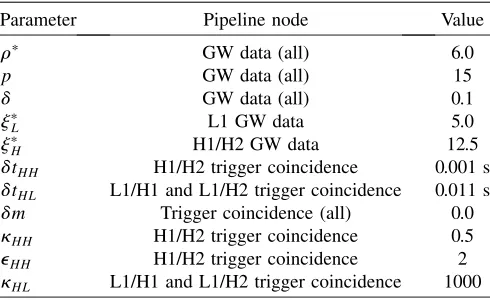
selected at the various stages of the pipeline. The procedures used to select these parameter values are outlined in the text.

Parameter Pipeline node Value

GW data (all) 6.0

p GW data (all) 15

GW data (all) 0.1

_L L1 GW data 5.0

H H1/H2 GW data 12.5

tHH H1/H2 trigger coincidence 0.001 s

tHL L1/H1 and L1/H2 trigger coincidence 0.011 s

m Trigger coincidence (all) 0.0

HH H1/H2 trigger coincidence 0.5

HH H1/H2 trigger coincidence 2

HL L1/H1 and L1/H2 trigger coincidence 1000 TABLE II. The effect of lowering the2threshold,, for the single interferometer L1, and for the combination of L1 and H1 in the pipeline. The efficiency of the L1 search remains constant as the threshold is lowered to 5.0; however, as the threshold is lowered in H1, the efficiency of the triggered search drops. Further testing indicated that a threshold of 12.5 in H1 was acceptable without a loss of efficiency.

Value of2_threshold,

L1 L1 efficiency Pipeline efficiency

20.0 0.350 0.270

15.0 0.350 0.270

10.0 0.350 0.255

Each strain waveform was calculated using the second order post-Newtonian expansion for an optimally oriented inspiral, and appropriately scaled for an inspiral at the desired effective distance. The strain was then converted into an injection signal into theyarm of the interferometer, with the appropriate calibration to produce the desired differential strain.

Of these injections, five sets were injected simulta-neously into all three instruments and the sixth was in-jected into L1 and H1 only. After the coincidence stage of the pipeline, 59 of the 60 injections produced a trigger in the appropriate template (1:4–1:4Mor1:0–1:0M). (The

single missed injection had a2 _{value in L1 which was}

slightly above threshold.) This is an excellent test of every stage of our pipeline. L1 successfully produced triggers corresponding to the injections, which were then used to make triggered banks against which the Hanford instru-ments were analyzed. Both H1 and H2 produced triggers which were coincident with those in L1. Furthermore, the amplitude cut between H1 and H2 was effective. For the louder injections, the effective distance was consistent between the two instruments. In the case of more distant injections which did not produce triggers in H2, the coin-cidence stage of the pipeline allowed the L1-H1 coincident triggers to be kept even though no event was found in H2. The pipeline was also run on an additional set of hard-ware injections at distances between 5 Mpc and 150 kpc. Of these injections, the most distant which produced coin-cident triggers were at 1.25 Mpc for the1:4–1:4M

injec-tion and 620 kpc for the 1:0–1:0M injection. This is

consistent with the sensitivity of H1 during the injection time, and with the efficiency measured in our software injections (Table I).

The trigger times associated with the hardware injec-tions all agreed with expectainjec-tions to within 1 msec.

Hardware injections provide a powerful test of instru-mental calibration. Any errors in the calibration of the instrument affect the measured effective distance to the inspiral. Uncertainties in distance measurements will con-tribute to errors in our detection efficiency. Additionally, they become important when requiring consistency of effective distance in triggers from the two Hanford instru-ments. To test the accuracy of the effective distance mea-surements, we used the loudest injections —namely the

1:4–1:4M injections with distances less than 100 kpc —

so that systematic errors in distance measurement would dominate over noise. The effective distance of all such injections was accurate to within 20%. We found that for L1, the distance to injections was systematically under-estimated by 5%, with a 4% standard deviation. For H1, there was a systematic underestimation of 2% with a standard deviation of 3%. For H2, we had a 2% over-estimation and a standard deviation of 5%. These errors are consistent with uncertainties in the calibration de-scribed in Sec. . Further details of the S2 hardware injec-tions are available in [32].

A Markov chain Monte-Carlo routine (MCMC) [33] was also used to examine the injected signals. This provides a method of estimating the parameters of an injected signal. As an example, for a1:4–1:4Minjection at 125 kpc, the

MCMC routine generated masses of 1:4003M and 1:3991M. The width of the 95% confidence interval for

each mass was0:012M.

VII. BACKGROUND ESTIMATION

An event candidate which survives all cuts in our analy-sis pipeline, including coincidence, can arise either from a real gravitational-wave signal or from noise bursts which contaminate our data streams. We refer to the latter class of event candidates as background. These background events are caused by many different environmental and instru-mental processes. Under the assumption that such pro-cesses are uncorrelated between the detectors at Hanford and Livingston, we estimated the rate for background events due to accidental coincidences by applying artificial time shiftstto the triggers coming from the Livingston detector. These time-shift triggers were then fed into sub-sequent steps of the pipeline. For a given time shift, the triggers that survived to the end of the pipeline represent a single trial output from our search (if no coincident gravitational-wave signals were present).

A total of 40 time shifts were analyzed to estimate the background:t 5,10,15,27,37,47,57,

67,77,87,97,107,117,127,137,147,

157,167,177,197seconds. To avoid correlations, we used time shifts longer than the duration of the longest template waveform (4 seconds). We did not time shift the triggers from the Hanford detectors relative to one another since real correlations may arise from environmen-tal disturbances. The resulting distribution of time-shift triggers in theH; L plane was used to determine a joint

signal-to-noise . Here L is given by Eq. (5) andH is

given by Eq. (9). For Gaussian noise fluctuations, with the single interferometer triggers’ SNR maximized over the polarization phase and the orbital inclination angle, one expects circular false alarm contours centered on the origin [34], suggesting that the sum of the squares of the signal-to-noise ratios would be a useful combined statistic. The time shifts revealed the need for a modified statistic; we settled on contours of (roughly) constant false-alarm probability to use in assigning a signal-to-noise to coinci-dent triggers. As shown in Fig. 7, the combined SNR

2

L2H=4 q

(10)

yielded approximate constant-density contours for the dis-tribution of background events in the plane.

result is shown in Fig. 8; the shaded bars represent the sample variance for ease of comparison with the zero-shift distribution. The apparent exponential dependence of

b on 2 _{further supports the choice of combined}

statistic in Eq. (10).

VIII. SEARCH RESULTS

The pipeline described above was used to analyze the S2 data. The output of the pipeline is a list of candidate coincident triggers. To decide whether there is any plau-sible detection candidate worth following up, we compare the combined SNR of the candidates with the expected SNR from the accidental background. If the probability of any candidate being accidental is small enough, we look at the robustness of the parameters of the candidate under changes in the pipeline, and we investigate possible in-strumental reasons for these candidates that may have been overlooked in the initial analysis.

Independently of whether detection candidates are found, we can use the results to set an upper limit on the rate of binary neutron star coalescences per Milky Way equivalent galaxy (MWEG), per year. We use the same statistics as in the previous search in S1 data [5], measuring the efficiency of the search at the SNR of the loudest trigger found. We take here the most conservative ap-proach, taking into account all triggers at the output of the pipeline: both those triggers considered to be potential detection candidates and those that are consistent with being due to instrumental noise or consistent with back-ground. We do not include the playground in the observa-tion time used for calculating the upper limit, since the playground was used to the tune the pipeline. This is consistent with our approach of focusing on detection, and not optimizing the pipeline for upper limit results (which was the reason for not considering single detector data, for example).

As described in Sec. II, after the data quality cuts, discarding science segments with durations shorter than 2048 s, and application of the instrumental veto in L1, a total of 373 hours of data were searched for signals, broken up in double- and triple-coincidence time as shown in Fig. 2. For the upper limit analysis, including the back-ground estimation, we only considered the nonplayback-ground times, amounting to 339 hours, of which 65% (221 hours) had all three detectors in operation; 26% (89 hours) had only L1 and H1 in operation; and 8.5% (29 hours) had only L1 and H2 in operation.

A. Triggers and event candidates

The output of the pipeline is a list of candidates which are assigned a SNR according to Eq. (10). There are 142 candidates in the nonplayground final sample with com-bined2 _{greater than 45; the breakdown is 90 candidates}

from L1-H2 two-detector data, 35 from triple-detector data, and 17 from L1-H1 two-detector data. All the candi-dates in the triple-detector data had SNR in H1 too small to cross the threshold in H2, and following our pipeline, were accepted as coincident triggers. Thus, all our coincident triggers are only double-coincidence candidates.

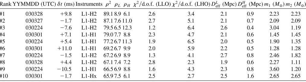
Table IV lists the ten largest SNR coincident triggers recorded in the analysis (including the playground).

ρ* 2

b(

ρ

*)

50 60 70 80 90 100

10−1 100 101 102

S2 final sample Expected background

FIG. 8. The number of triggers per S2 above combined SNR

. The triangles represent the expected (mean) background based on 40 time-shift analyses. The shaded envelope indicates the sample variance in the number of events. The choice of combined SNR in Eq. (10) is further justified by the behavior

b /exp2 _{down to about 0.3 events per S2. The circles}

represent the unshifted inspiral event candidates (Sec. VIII A). FIG. 7 (color online). The signal-to-noise at Livingston L

plotted against the signal-to-noise at Hanford H for triggers

Detailed investigations of the conspicuous triggers were performed and are reported below. Nine out of these ten candidates were in the double-detector sample. There was only one (#10 in the list) which was in the triple-detector data, although it was too weak to require a corresponding trigger in H2. Our loudest candidate, as well as five of our loudest ten, are L1-H2 coincident triggers; in fact, 63% of all our candidates are L1-H2 coincident triggers. Since the L1-H2 data supplies only 9% of the total observation time, we conclude that the noise in H2 was significantly different than the noise in H1, producing more and louder triggers. For all triggers in Table IV, the effective distance is larger in the Livingston detector than in the Hanford detector: although this is plausible for real signals, as shown in Fig. 6, it suggests that these candidates are more likely to originate from instrumental noise.

A trigger gets elevated to the status of an event candidate if the chance occurrence due to noise is small as deter-mined by time-shift background estimation, calculated as described in Sec. VII. Each event candidate is subjected to follow-up investigations beyond the level of automation used in our pipeline to ensure that it is not due to an instrumental or environmental disturbance.

In Fig. 8, a cumulative histogram of the final coincident triggers versus2_{is overlayed on the expected background}

due to accidental coincidences, as determined by time shifts. Even after taking into account that these are cumu-lative histograms, so that adjacent bins are strongly corre-lated, it appears that the number of coincident triggers is inconsistent with the expected background for large 2_.

While the origin of this discrepancy is not understood, careful examination of the three coincident triggers with the highest2_{, detailed below, indicates that these are not}

gravitational-wave detections. Moreover, no evidence of correlated noise between the Livingston and Hanford ob-servatories was found for times around these triggers. In Sec. VIII B, we demonstrate that a reasonable modification

of our algorithm for clustering multiple coincident triggers results in good agreement between the coincident trigger sample and the background estimate. This shows that the background estimate is not robust with respect to reason-able variations in the analysis procedure.

In Sec. IX we derive an upper limit on the rate of inspiral events which is conservative with respect to any uncertain-ties in the background estimate. Thus, although the dis-crepancy between the coincident triggers and the background estimate presented in Fig. 8 is not understood, it does not affect our ability to detect inspiral signals or set an upper limit on the inspiral rate.

1. Trigger 030328

The loudest candidate is in a cluster of three coincident triggers in L1 and H2 on March 28, 2003. The loudest trigger in the cluster, #1 in Table IV, has a large SNR in L1 (8:9), but a SNR in H2 (6:1) which is close to threshold for trigger generation. We expect a candidate arising from a real signal to be robust under small changes in our analysis pipeline. In order to test the robustness of this particular candidate upon changes in the boundaries for the blocks used in the analysis, we reanalyzed the data in this science segment shifting the start time of the block by different amounts in L1 and H2. Although in all cases our analysis produced similar numbers of triggers in each detector, only in the original case were there triggers within 11 ms that had identical masses and were considered candidates.

Other measured parameters of this trigger reinforce the conclusion that it should not be promoted to a detection candidate. The2_{per degree of freedom is bad, especially}

in H2 (3.4); the2_{in L1 is close to our threshold [}2_=p

22 _{4:6 compared to the threshold 5]. The}

ef-fective distances measured by the detectors are very differ-ent, 2.1 Mpc in L1 and 0.9 Mpc in H2. This ratio of

TABLE IV. The 10 triggers with the largest SNR which remain at the end of the pipeline. This table indicates their UTC date, the time delay between Hanford and Livingston (ttHtL), the combined SNR2 [from Eq. (10)], the SNR registered in each detector, the value of 2 _{per degree of freedom at each interferometer (for 2p228 d:o:f:), the effective distance to an}

astrophysical event with the same parameters in each detector, and the binary component masses of the best matching template (identical for the triggers in both detectors). The notation L1-Hx means that all three interferometers were in science mode at the time of this coincident trigger.

Rank YYMMDD (UTC)t(ms) Instruments 2 L H 2=d:o:f:(LLO)2=d:o:f:(LHO)DLeff (Mpc)D H

eff (Mpc)m1(M)m2(M)

#1 030328 9:8 L1-H2 89.1 8.9 6.1 2.6 3.4 2.1 0.9 2.23 2.23

#2 030327 1:7 L1-H2 87.1 7.6 11.0 2.7 5.1 2.1 0.7 2.09 2.09

#3 030224 7:6 L1-H2 79.5 6.5 12.3 1.2 6.4 2.6 0.4 3.04 1.19

#4 030301 7:1 L1-H1 79.0 7.7 8.8 2.3 4.7 2.1 0.6 1.45 1.45

#5 030224 5:4 L1-H1 77.2 6.7 11.3 1.9 6.5 2.0 0.5 1.90 1.35

#6 030301 11:0 L1-H1 69.2 6.7 9.9 2.0 5.9 2.2 0.5 1.28 1.28

#7 030224 1:5 L1-H2 67.2 6.9 8.9 1.3 4.1 2.7 0.8 2.46 1.82

#8 030328 4:4 L1-H2 67.1 7.4 7.2 2.8 2.3 1.9 0.6 2.27 1.11

#9 030224 10:5 L1-H1 66.5 6.9 8.8 1.6 4.3 2.3 0.8 3.60 1.20

#10 030301 1:7 L1-Hx 65.9 7.5 6.1 2.5 2.7 2.5 1.6 2.65 2.65