A Novel Approach for Robust Maximum Power Point Tracking of PEM Fuel Cell Generator Using Sliding Mode Control Approach

Int. J. Electrochem. Sci., 7 (2012) 4192 - 4209

International Journal of

ELECTROCHEMICAL

SCIENCE

A Novel Approach for Robust Maximum Power Point Tracking

of PEM Fuel Cell Generator Using Sliding Mode Control

Approach

Sh. Abdi, K. Afshar*, N. Bigdeli, S. Ahmadi

Advanced Power and Control Systems Lab., EE Department, Imam Khomeini International University, Qazvin, Iran

*

E-mail: [email protected]

Received: 20 February 2012 / Accepted: 6 April 2012 / Published: 1 May 2012

In this paper a fast and efficient maximum power point tracking (MPPT) control scheme for PEM fuel cells is proposed which is based on sliding mode control approach. The closed loop system includes the PEM fuel cell, boost chopper, battery and sliding mode controller. Sliding mode controller is used to control the duty cycle of the chopper in order to achieve MPPT. The characteristics of the approach are its good transition response, low tracking error, very fast system reaction against set point, fuel cell temperature and membrane water content, robustness as well as low complexity. The performance and accuracy of the proposed algorithm has been investigated in different situations and compared with Perturb and Observe algorithm.

Keywords: PEM Fuel Cell; Robust control; Maximum Power Point Tracking (MPPT); Sliding Mode Control; Perturb and Observe.

1. INTRODUCTION

become the most popular type of fuel cells and the best candidate for residential and vehicular applications [1, 2].

Fuel cell output power depends on the applied current or voltage and fuel cell output voltage is dependent on operating conditions, including cell temperature, air pressure, oxygen partial pressure, and membrane water content [3]. Fuel cells have nonlinear voltage-current characteristic, and there is only one unique operating point for a fuel cell system with a maximum output under a particular condition. However, the maximum power point (MPP) varies with temperature and membrane water content. Therefore, the maximum power point tracking (MPPT) at all operating conditions is a challenging problem. In fact, in the MPPT algorithm, the stack current and fuel flow are controlled under various operating conditions to optimize fuel consumption and the extract maximal power of the fuel cell [3].

There are different methods for MPPT in the literature. A good study about different MPPT methods such as Hill-climbing/ Perturb and Observe (P&O), incremental conductance, fractional open-circuit voltage, fractional short-open-circuit current, fuzzy logic control, neural network, ripple correlation control , current sweep, DC-Link capacitor droop control, load current or load voltage maximization, sliding mode control approach and other MPPT techniques for photovoltaic system may be found in [4]. MPPT methods vary in complexity, implementation hardware, popularity, convergence speed and sensed parameters [4]. Many MPPT methods have been applied to fuel cell for exacting maximum available powers from fuel cell modules, e.g., P&O [5-9], adaptive MPPT control [10], motocompressor control technique [11], adaptive fuzzy logic controller [12], MPPT algorithm based on resistance matching between the direct methanol fuel cells internal resistance and the tracker’s input resistance [13], voltage and current based MPPT [14], adaptive extremum seeking control [15]. This paper proposes a fast and robust MPPT control scheme based on sliding mode control (SMC) for PEMFC system. The characteristics of the approach are its good transition response, low tracking error, very fast system reaction against set point, fuel cell temperature and membrane water, robustness as well as its low complexity. The performance and accuracy of the proposed algorithm has been investigated in different situations and compared with Perturb and Observe algorithm of [10].

This paper is organized as follows: The problem formulation is presented in section 2. The proposed MPPT control algorithm is presented in section 3. In section 4, the simulation results are given, analyzed and discussed. Finally, the conclusions are presented in section 5.

2. PROBLEM FORMULATION

variable for the achieving MPPT. V_O is the output voltage and i_L is the inductor current. It is assumed that i_Lis equal to the FC current (i_FC). The FC output voltage is given as [6, 10, 14, and 16]:

cell Nernst act ohm conc

V E V V V (1)

Where,E_Nernst is the reversible (or open-circuit) thermodynamic potential his is described by the Nernst equation as:





4 5

1.229 8.5 10 ( 298.15) 4.308 10 ln( ) 0.5ln( )

Nernst H O

E     T    T P  P (2)

Where T is the absolute temperature ( K ),

2 H

P is the hydrogen partial pressure (atm) and

2 O P

the is oxygen partial pressure (atm). Activation voltage drop is given in the Tafel equation as:

2

1 2 3 ln( ) 4 ln( )

act O FC

V   T T C  T I

(3)

Where the _i parameters, i = 1,…,4, are parametric coefficients for each cell model, and

2 O

C represents the dissolved oxygen concentration in the interface of the cathode catalyst which can be calculated as:

2

2 _{(5.08 10 ) exp( 498}6 ₎ O

O

P C

T 

   (4)

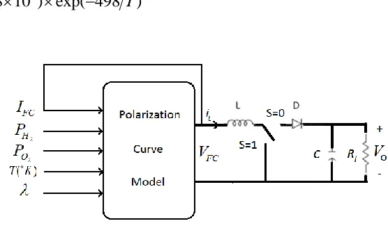
Figure 1. PEMFC generator system. The overall ohmic voltage drop can be expressed as:

ohmic FC M

V I R (5)

m m M

r t R

A 

(6)

Where, t_m is the membrane thickness (cm), A is the activation aria and r_m is the membrane resistivity(cm)to proton conductivity. Membrane resistivity depends strongly on membrane humidity and temperature and can be calculated as:





2 2.5

181.6 1 0.03( ) 0.0062( 303) ( )

0.634 3( ) exp(4.18( 303 ))

FC Fc

m

m FC

I A T I A

r

I A T T



   

 



   (7)

Where, _m represent the water content of the membrane and is an input of PEMFC model. The membrane water content_m is a function of the average water activitya_m:

2 3

0.043 17.81 39.85 36 , 0 1

14 1.4( 1),1 3

m m m m

m

m m

a a a a

a a

 _{ }     

   

 (8)

The average water activity is function of the anode water vapor partial pressure P_{v an,} and the cathode water vapor partial pressureP_{v ca,} and can be expressed as:

, ,

1 1

( )

2 2

v an v ca m an ca

sat

P P

a a a

P 

   (9)

The saturation pressure of water P_sat can be figured out with the following empirical expression:

5 2 7 3

10 sat 2.1794 0.02953 9.1813 10 1.4454 10

lpg P    T   T    T (10)

The real values of _m that can vary from 0 to 14, which is equivalent to a relative humidity of 0%-100%. However, under supersaturated conditions it can be as high as 23. The concentration voltage drop is expressed as:

ln(1 FC)

conc

L I RT

V

nF i A

   (11)

Where, iL is the limiting current. It denotes the maximum rate at which a reactant can be supplied to an electrode.

The voltage and therefore, the power of one Fuel cell is limited, and thus, Fuel cells are connected with each other in series for achieving the suitable and appropriate voltage. The nonlinear V–I equation characteristic of N_FC series cells per string is:

FC FC cell

The

FC

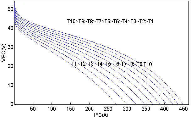
P -I_FC characteristic of Fuel cell in different temperatures has been shown in Fig.2 and the

FC

V -I_FC characteristic of Fuel cell in different temperatures is shown in Fig.3. These curves show that the output power of the Fuel cell array is a nonlinear function of current and strongly influenced by the cell temperature. Each curve has a MPP at which the sola Fuel cell array operates with the highest efficiency. This numerical modeling shows the importance of use of a MPPT algorithm.

Figure 2. The

FC

P - I_FC characteristic of Fuel cell in different temperatures

Figure 3. The

FC

V - I_FC characteristic of Fuel cell in different temperatures.

3. STATE SPACE MODEL OF BOOST CONVERTER

1

( )

FC L O L

V i V

i

L L

  ₍₁₃₎

1

O L O

L V i V

C CR

 

(14) If the switch is in positionS 1, the differential equation can be written as:

2

( )

FC L L

V i i

L

 ₍₁₅₎

2

O O

L V V

CR  

(16)

Using the state space averaging method [17], Eqs.(13) to (16) can be combined into one set of state space equations to represent the dynamic of the system. Based on the idea of Pulse-Width Modulation (PWM), the ratio of the switch in position 1 in a period is defined as the duty ratio. Two distinct equation sets are weighted by the duty ratio and superimposed as:





X  D X DX

(17) Where:

1 1

1

T L O X  i V _

(18)

2 2

2

T L O X  i V _

(19) Hence, the dynamic equation of the system can be described as:

( )

 FC L  O  O

L

V i V V

i D

L L L (20)

 L  O  L

O

L V

i i

V D

C CR C (21)

Where, D

 

( ) ( )

X  f X g X D

(22)

4. MPPT OF PEMFC BASED ON SLIDING MODE CONTROL

cross-section of the system’s normal behavior [18]. SMC discussed first in the Soviet literature and have been widely developed in recent years [18]. One application of sliding mode controllers is the control of electric drives operated by switching power converters. Because of the discontinuous operating mode of those converters, a discontinuous sliding mode controller is a natural implementation choice over continuous controllers that may need to be applied by means of pulse-width modulation or a similar technique of applying a continuous signal to an output that can only take discrete states. This paper proposes a fast MPPT control scheme based on SMC for PEMFC system.

The operation modes of sliding mode control include two modes: approaching mode and sliding mode. We define the sliding surface as follows [19]:

0

FC FC P I 



 (23)

It will be shown that by selecting the sliding surface as in Eq. (23), it is guaranteed that the system state will hit the surface and produce maximum power output persistently.

( )

0

FC FC FC FC

FC FC

FC FC FC

P V I V

V I

I I I

  

   

   (24)

Hence, the sliding surface is defined as: FC

FC FC FC V

V I

I

  

 (25)

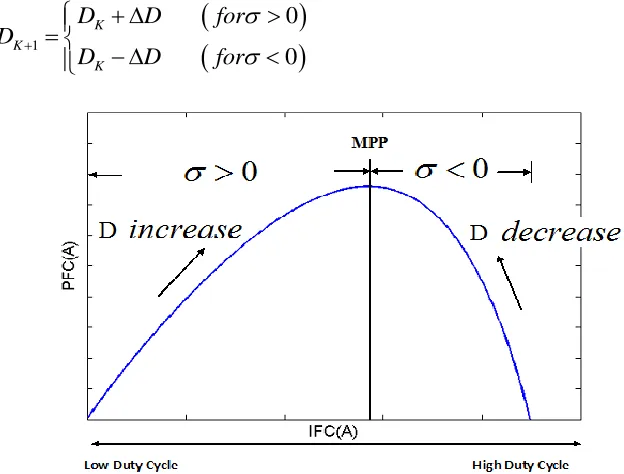
The duty cycle (D) output control (according to Fig.4) based on the observation of duty cycle versus operation region can be chosen as:









1

0

0

 



   

  

  

 K K

K

D D for

D

D D for (26)

Where, The equivalent control (D_K) is determined from the following condition:

( )

1 FC FC

K

O V i D

V

  (27)

Note that in this case, i_Lis assumed to be equal to the fuel cell current (i_FC) (The equivalent series resistance of the inductor and wiring resistance of boost converter are neglected). A Lyapunov function is now defined as:

2

1 :

2 

V (28)

The time derivative of  can be written as:





2

2

( )

2 FC FC O 1 FC FC

FC L FC

FC FC FC FC

V V V V i

I I I D

I I I I L L

 

     _    _   _

  _   _{ } (29)

Where V_FC I_FC and 2 2

FC

FC

V I

  can be calculated as:

( )

FC act ohm con FC

FC FC FC FC

V V V V

N

I I I I

   

   

    (30)

( )

FC act m con

FC m FC

FC FC FC FC

V V R V

N R I

I I I I

 

 _{ }  _{ }  _

 

 _   _ (31)

2 2 2 2

2 2 2 ( 2 ) 2

FC FC

FC act m m con

FC FC

FC FC FC I I

V V R R V

N I

I I I

 

 _{ }  _  _  _

 

 

 _     _ (32)

Where,Vact IFC,

2 2

 

FC

act

V I , Vcon IFCand

2 2

 

FC

con

V I can be calculated as:

4 act FC FC V T I I   

 (33)

2 4 2 2 FC FC act V T I I      (34) 1 con

FC L FC

V RT

I nF i A I

 

 _

 

 _  _ (35)

2 2 2 1 ( ) FC con L FC V RT

I nF i A I

 

 _

 

 _  _ (36)

2 1 3 m K R K K

 (37)

1 181.6 303 exp 4.18 m t K T A T         (38) 2 2.5

2 1 0.03( FC ) 0.0062( 303) ( Fc )

K   I A  T I A (39)

3 0.634 3

FC m I K A      _{  }

  (40)

3

2 2

3 2 3 2

1 2 1 2

3 3

3

( ) ( )

FC FC FC

m FC

K

K K

K K K K

I I I A

R

K K

I K K

  _     _  

 _{ }   _ 

 _{     }

 (41)

2 2

2 2 2

3 2 3 2

2

1

2 3

3

3 3

( ) 2 2

( )

FC FC

m FC

K K

K K K

I A I A

R K I K  _{    }     _{ }   _{   }   _{  }

 (42)

1.5 2

2 0.03 2.5

0.062 303 FC FC I K T

I A A A

 _{ }     

    

      (43)

0.5 2 2 2 2 2.5 1.5 0.062 303 FC FC I K T

I A A A

 _      

     

       (44)

3 3

FC K

I A

 _ 

 (45)

Substitution of Eqs.(31) and (32) into Eq.(29) yields:

2

2

2 FC FC 0

FC

FC FC FC

V V

I

I I I

    

 _{  }

 

 _   _ (46)

The signs of Eqs.(33), (35) to (44) are positive and Eqs. (34) and (45) are negative. Because, the 2 2 act FC V I 

 value is very small with respect to the other parameters in Eqs. (31) and (32). Therefore, according to the above mentioned equations, the Eqs. (31), (32) and (46) negative definite.

As stated, by zero sliding surface (i.e.  0) the maximum power output production in the system is guaranteed. The achievability of  0 will be obtained by  0 for all D discussed as follows:

Since the range of duty cycle must lies in 0D_eq 1 the real control signal is proposed as:













1

1 1 0 1 0 1

         _      _{ }  K

K K K

K

D K

D D K D K

D K

(47)

Where, K is a positive scaling constant K can be considered as the effort to track the MPP. From Eqs. (20), (27), (29) and (47) on can write:









O FC FC

L

O FC FC

K

O FC FC FC FC

O O

V V i

I D

L L

V V i

D k

L L

V V i V i

k

L V L

V K L                   _    _      (48)

Therefore, based on Eqs. (46) and (48),  always has inverse sign of . Therefore,  0 is obtained. for0 D 1.

2) D1

For D1 it can be written:

( ) 0 FC FC L V i I L

  (49)

Based on Eqs. (46) and (49),  0. ForD1, two cases should be inquired for the fulfillment of 0:

2.a) D_k 1 and D_kK 0

Which means the system is operating at the left-hand corner of Fig.4. According to Fig.4 If the system is operated at the left-hand corner,  is positive. Therefore, D_K K will be increasing. 2.b) D_k 1

Which means the system is operating at the right-hand corner of Fig.4. If the system is operated at the right-hand corner,  is negative. Therefore, D_K K will be decreasing. It concludes that

0

  forD1.

For D0, it can be written that:

( )

0

O FC FC L

V V i

I

L L

 

 _  _

  (50)

Since boost converter is used in conjunction with the Fuel cell, in this paper, in this case the output voltage (V_O) is higher than the input voltage (V_FC). Therefore, from Eqs. (46) and (50), it is resulted that  0. ForD0, two cases are examined as follows:

3.a) Dk 0

Which means the Fuel cell module is directly connected to the load and operates in the region

0

  . Therefore, D will be increased and it contradicts to the assumption of D0. 3.b) D_k 0 and D_kK 0

In this case,  0is obtained and 0. It concludes that  0forD0.

The above statements can be summarized as follows: according to Fig.3, if the system is operated at the left-hand corner,  will be positive. Therefore, DK K will be increasing. If the system is operating at the right-hand corner,  is negative for this case. Therefore, DK K will be decreasing. Besides, if system is operated at MPP, then is zero and DK1=DK. Thus, as mentioned above, the asymptotic convergence to the MPP state (i.e.  0) can be guaranteed using the proposed control law in Eq.(47).

5. SIMULATION RESULTS

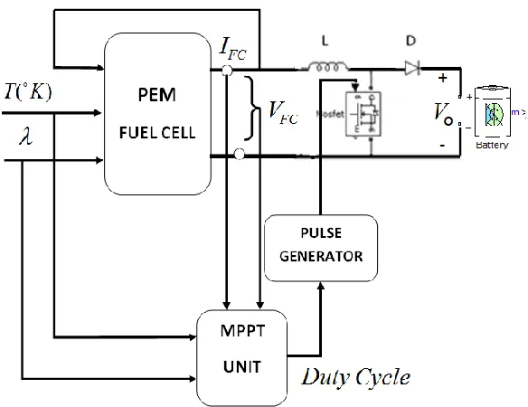
In order to investigate the performance and accuracy of the proposed MPPT method, simulations are performed for three different cases in MATLAB/SIMULINK for different situations including normal operating conditions and fast variation of the cell temperature and the membrane water content. The configuration of the studied PEMFC system in this paper has been shown in Fig. 5. It includes a PEMFC, boost DC/DC converter, a battery and control system. The duty cycle of the boost DC/DC converter is the only control variable for achieving MPPT.

The properties of the used model of PEMFC are presented in the Appendix A. Besides, the proposed method has been compared with the presented P&O algorithm in [10].

5.1. Case study I: Normal operating conditions

Figure 6. The time evolution of

FC

P under normal operating condition (11 andT 343 K).

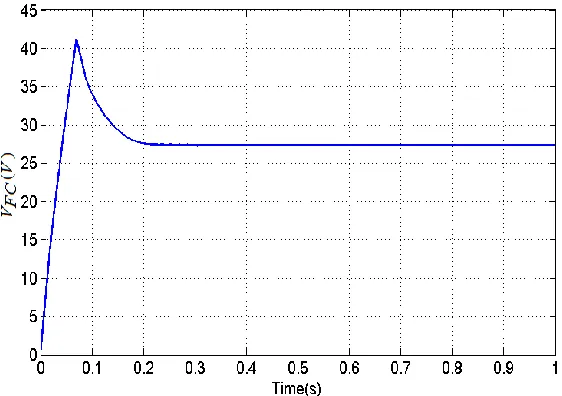
Figure 7. The time evolution of

FC

Figure 8. The variation of

FC

P versus I_FC under normal operating condition (11 andT 343 K).

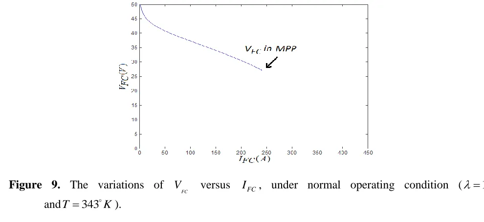
Figure 9. The variations of

FC

V versus I_FC, under normal operating condition (11

andT 343 K).

In this case, it has been assumed that, the membrane water content  and temperature T is constant. The value of  is considered 11 and the value of temperature is considered 343 K . The optimal power corresponding to this  and T is 6.625 kW. Simulation results for this case study are shown in Figs.6 to 9. In this case, the simulations are done for the proposed MPPT method. Figs.6 and 7 show the time evolution of

FC

P and

FC

V , respectively. Figs.8 and 9 show the variations of

FC

P and

FC

V versus I_FC, respectively, under the normal operating condition. As seen in this figures,

FC

P has been converged to the desired set point in a settling time of 0.2 sec with about 1.% error. Besides, the values of

FC

V and I_FC remain bounded and reasonable, for this case.

5.2. Case study II: Fast variation of the Fuel Cell temperature

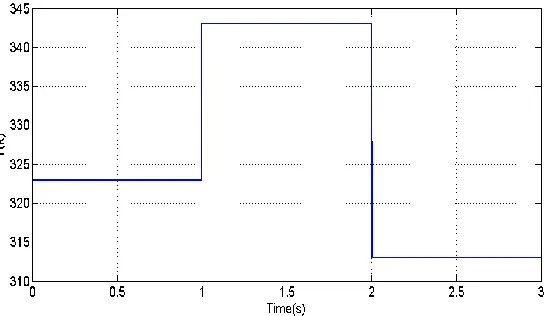
temperature in the constant membrane water content, a step change is applied to the temperature. In this case we assume that the membrane water content is 11. The system is at first operating in the temperatureT 323 K. At this temperature, the optimal power is 5.632 kW. At t = 1 s, the temperature is increased to 343 K. The optimal power corresponding to this temperature is 6.625kW. Once again, at t = 2 s, the temperature is decreased to313 K. At this temperature, the optimal power is 5.130kW. Simulation results for this case study are shown in Figs. 10 to13. The simulations the proposed MPPT method (sliding mode) are compared for P&O method presented in [10].

Fig. 10 shows the time evolution of the variable temperature and in Figs. 11 and 12, the variations of

FC

P and

FC

V versus I_FC, are illustrated, respectively. The time evolution of

FC

P has been also brought in Fig. 13. Besides, the performance of the proposed MPPT method (sliding mode) has been compared with well-known and P&O method [10] in Fig. 13. Table 1 presents the numerical comparison between the proposed MPPT approach and the P&O approach in [10] under fast variation of the Fuel Cell temperature in constant membrane water content. From these results one can conclude that the proposed sliding control has been able to make the closed loop system to reach the new set points caused by the variation of the fuel cell temperature, satisfactorily.

Figure 10. Time variations of cell temperature.

Figure 11. The variations of

FC

Figure 12. The variations of

FC

V versus I_FC, under fast variation of the Fuel Cell temperature in constant membrane water content (11).

Figure 13. The time evolution of

FC

P under fast variation of the Fuel Cell temperature in constant membrane water content ( 11) for both the proposed and the P&O [10] methods.

Small settling time, no overshoot, and steady error of about 1% are the good features of the proposed MPPT method.

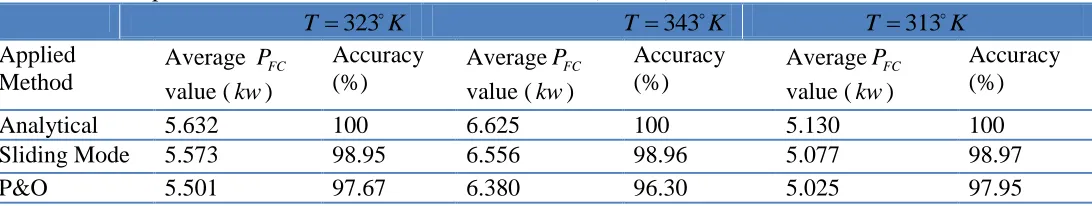
Table 1. Comparison of Sliding Mode and P&O approaches results under fast variation of the Fuel cell temperature in constant membrane water content (11).

313

T  K

343

T  K

323

T  K

Accuracy (%) AverageP_FC

value (kw) Accuracy

(%) AverageP_FC

value (kw) Accuracy

(%) Average P_FC

value (kw) Applied

Method

100 5.130

100 6.625

100 5.632

Analytical

98.97 5.077

98.96 6.556

98.95 5.573

Sliding Mode

97.95 5.025

96.30 6.380

97.67 5.501

5.3. Case study III: Fast variation of the Fuel Cell membrane water content.

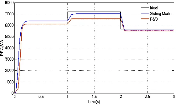
The performance of the proposed MPPT method under variation of cell membrane water content in constant temperature has been investigated in this section, too. For this purpose, a step change is applied to the membrane water content. In this case it is assumed that the temperature is323 K. The system is first operating at13. At this, the optimal power is 6.441 kW. At t = 1 s,  is increased to 15. The optimal power corresponding to this  is 7.179kW. Again, at t = 2 s,  is decreased to 11. At this, the optimal power is 5.632kW. Simulation results for this case study are shown in Figs.14 and 15. The simulation is done for the proposed MPPT method (sliding mode) and P&O method [10], as well.

Figure 14. Time variations of membrane water content.

Figure 15. The time evolution of

FC

P under fast variation of the membrane water content in constant temperature (T 323 K) for both the proposed and the P&O [10] methods.

The membrane water content variations have been shown in Fig. 14 and the time evolution of

FC

content in constant Fuel Cell temperature has been presented. The results show that the proposed MPPT method has high accuracy and reliability in comparison with the P&O method [10], in tracking of the maximum power point in different membrane water content. Small settling time, no overshoot, and steady error of about 2% are the good features of the proposed MPPT method.

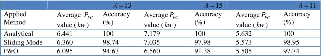
Table 2. Comparison of Sliding Mode and P&O approaches results under fast variation of the membrane water content in constant temperature (T 323 K).

11



15



13



Accuracy (%) AveragePFC

value (kw) Accuracy

(%) AveragePFC

value (kw) Accuracy

(%) Average PFC value (kw) Applied

Method

100 5.632

100 7.179

100 6.441

Analytical

98.95 5.573

97.98 7.035

98.74 6.360

Sliding Mode

97.74 5.505

91.38 6.560

94.63 6.095

P&O

6. CONCLUSIONS

In this paper, a sliding mode based maximum power point tracking approach for PEM fuel cell is presented and its characteristics, accuracy and performance is investigated via simulations. The analyses and simulations are performed on a system including of a PEMFC, boost DC/DC converter and a battery for both normal and time varying Fuel cell temperature and membrane water content operating conditions. Besides, the performance of the proposed method is compared with the P&O approach [10]. The results are indicative of the out performance of the proposed method. The main features of sliding mode MPPT method can be summarized as:

 High accuracy or equivalently low steady state tracking error;  Fast response;

 Simple control law, low complexity and implementation cost.

Appendix A: Characteristics of studied PEMFC system.

F (Faraday’s constant) 96484600 (C kmol1) R (Universal gas constant) 8314.47 (Jkmol1 K)

FC

N (Number of Cells) 35

A (Cell active area) 232 (cm2)

2 H

P (Hydrogen partial pressure) 3 (atm)

2 O

P (Oxygen partial pressure) 1 (atm)

1

 (Semi empirical coefficient) 0.944

2

 (Semi empirical coefficient) -0.00354

3

4

 (Semi empirical coefficient) 4

1.96 10 

L

i (Limiting current) 2 (Acm2 )

References

1. J.M. Andujar, F. Segura, Renew. Sustai. Energ. Rev. 13 (2009) 2309–2322. 2. X. Zhang, J. Guo, J. Chen, Energy 35 (2010) 5294-5299.

3. J.O. Schumacher, P. Gemmarb, M. Denneb, M. Zedda , M. Stueber, J. Pow. Sour. 129 (2004) 143–151.

4. T. Esram and P.L. Chapman, IEEE Trans. Energ. Conv. 22:2 (2007) 439-449.

5. L. N. Khanh, J.J Seo, Y.S Kim, and D.J Won, IEEE Trans. Energ. Conv. 25:3 (2010) 1874-1882. 6. A. Giustiniani, G. Petrone, G. Spagnuolo, and M. Vitelli, IEEE Trans. Energ. Conv. 57:6 (2010)

2042-2053.

7. C.A.R. Paja, G. Spagnuolo, G. Petrone, R. Giral and A. Romero, IEEE Int. Symp. Circ. Syst. (2010) 2199-2202.

8. M. Dargahi, M. Rezanejad, J. Rouhi and M. Shakeri, IEEE Int. Mult. Conf. (2009) 33-37.

9. L. Egiziano, A. Giustiniani, G. Petrone, G. Spagnuolo, M.Vitelli, IEEE Int. Conf. Clean Elec. Pow. (2009) 775– 781.

10.Z. Zhi-dan , H. Hai-bo , Z. Xin-jian , C. Guang-yi , R. Yuan, J. Pow. Sour. 176 (2008) 259–269. 11.M. Becherif , D. Hissel, Int. J. Hydr. Energ. 35 (2010) 12521-12530.

12.N. Chanasut and S. Premrudeepreechacharn, IEEE Ind. Appl. Soc. Ann. Meet. (2008)1–6. 13.K.H. Loo, G.R. Zhu, Y. M. Lai, and C. K. Tse, 8th Int. Conf. Pow. Elect. (2011)1753-1760. 14.M. Sarvi, M.M. Barati, IEEE Pow. Eng. Conf. (2010) 1-4.

15.N. Bizon, Appl. Energ. 87 (2010) 3115–3130.

16.L. N Khanh, J. J Seo, Y. S Kim, and D. J Won, IEEE Trans. Pow. Deliv. 25: 3 (2010) 1874 – 1882.

17.R.W. Erickson and D. Maksimovic, Fundamentals of Power Electronics, Kluwer Academic Publishers, 2001.

18.Y.A. Mohammed , E.H. Karam and M.H. Khudair , Eng. Tech. J. 27:12 (2009) 2494-2505. 19.Ch. Ch. Chu, Ch. L. Chen, Solar Energ. 83 (2009) 1370–1378.