City, University of London Institutional Repository
Citation:
Starnini, M., Baronchelli, A. and Pastor-Satorras, R. (2012). Ordering dynamics of the multi-state voter model. Journal of Statistical Mechanics: Theory and Experiment new, 2012(10), doi: 10.1088/1742-5468/2012/10/P10027This is the unspecified version of the paper.
This version of the publication may differ from the final published
version.
Permanent repository link:
http://openaccess.city.ac.uk/2668/Link to published version:
http://dx.doi.org/10.1088/1742-5468/2012/10/P10027Copyright and reuse: City Research Online aims to make research
outputs of City, University of London available to a wider audience.
Copyright and Moral Rights remain with the author(s) and/or copyright
holders. URLs from City Research Online may be freely distributed and
linked to.
Michele Starnini1, Andrea Baronchelli2, and Romualdo
Pastor-Satorras1
1Departament de F´ısica i Enginyeria Nuclear, Universitat Polit`ecnica de Catalunya,
Campus Nord B4, 08034 Barcelona, Spain
2Laboratory for the Modeling of Biological and Socio-technical Systems,
Northeastern University, Boston MA 02115 USA
Abstract. The voter model is a paradigm of ordering dynamics. At each time step,
a random node is selected and copies the state of one of its neighbors. Traditionally, this state has been considered as a binary variable. Here, we address the case in which the number of states is a parameter that can assume any value, from 2 to∞, in the thermodynamic limit. We derive mean-field analytical expressions for the exit probability, the consensus time, and the number of different states as a function of time for the case of an arbitrary number of states. We finally perform a numerical study of the model in low dimensional lattices, comparing the case of multiple states with the usual binary voter model. Our work sheds light on the role of the parameter accounting for the number of states.
PACS numbers: 89.65.-s, 05.40.-a, 89.75.-k
1. Introduction
Models of ordering dynamics have since long been considered as paradigms of opinion
dynamics and consensus formation in social systems (1). Most of them share the
fundamental feature that order results from the self-organization of local and usually short-range pairwise interactions between agents, as it is well illustrated by the simplest and most analyzed of them, the so-called voter model (2; 3). In its basic formulation, the voter model is defined as follows: Each individual in a population (agent) is endowed with a binary spin variable, representing two alternative opinions, and taking values
σ =±1. At each time step, an agent i is selected at random together with one nearest
neighbor j and the state of the system is updated as σi :=σj, the first agent copying
the opinion of its neighbor. Starting from a disordered initial state, this dynamics leads in finite systems to a uniform state with all individuals sharing the same opinion (the so-called consensus).
From the point of view of social dynamics, the interest in this kind of models is mainly focused on the way in which consensus is reached. The approach to this state
is characterized in terms of the exit probability E(x) and the consensus time TN(x),
defined as the probability that the final state corresponds to all agents in the state +1
and the average time needed to reach consensus in a system of size N, respectively,
when starting from a homogeneous initial condition with a fraction x of agents in state
+1 (1). Due to its simplicity, the voter model dynamics can be exactly solved in regular lattices for any number of dimensions (4; 5). Thus, considering the average conservation
of magnetization m = PN
i=1σi/N, it can be shown that the exit probability is always
a linear function, E(x) = x. On the other hand, the consensus time starting from
the homogeneous symmetric initial condition x = 1/2 scales with system size N as
TN(1/2) ∼ Neff, with Neff ∼ N2 in d = 1, Neff ∼ NlogN in d = 2, and Neff ∼ N in
d >2 (at the mean-field level) (5). Finally, the dependence of consensus time with the initial density of +1 spins, starting from homogeneous initial conditions, takes the form
TN(x) =−Neff[xln(x) + (1−x) ln(1−x)], (1)
for d≥2 (6).
Different variants of the voter model have been considered in the past, including the presence of quenched disorder in the form of “zealots” which do not change opinion (7; 8), memory and noise reduction (9), inertia (10), conservative voters (11), non-linear interactions (12; 13), etc.; see Ref. (1) for an extended bibliography on this subject.
A variant that has been considered in several contexts is the multi-state voter model,
in which each agent can be in one ofS different exclusive states or opinions, in analogy
multi-state voter model, introducing non-equivalent states, have also been discussed in the literature (21; 22; 23).
In this paper we focus in the study the ordering dynamics of the symmetric multi-state voter model, focusing in particular on the limit of a large number of initial multi-states.
Each agent can be in one ofS different but dynamically equivalent states. Agents follow
the same dynamical update rules than in the binary version, with time being update
at every dynamical step as t → t + 1/N. Expressions for the consensus time in this
model at the mean-field level have already been provided in the literature (24; 25; 26). The derivations presented so far rely however on heavy mathematics. Here, building on the Fokker-Planck formalism presented in Ref. (27), we rederive in a simple way the
expressions for the exit probability and the consensus times in the general case of S
states. We find that the consensus time increases very slowly with the number of states,
and its difference with the binary case saturates asS → ∞; we rationalize this finding by
comparing it with the case of the mutant invasion in the ordinary two-state voter model. We also investigate the decay of the number of states as a function of time, providing a mean-field expression in excellent agreement with simulations. We finally consider the dynamics of the multi-state voter model on low dimensional lattices. Lacking of specific analytical insights, we compare the numerically observed phenomenology to the mean-field case, and point out similarities and differences, focusing on the effect of the number of initial states and their configuration.
The paper is structured as follows. Sec. 2 is devoted to the analysis of the mean-field multi-state voter model. Sec. 3 reports on numerical experiments concerning the low-dimensional case. Finally, Sec. 4 presents our conclusions.
2. Mean-field analysis
The form of the consensus time in the multi-state voter model at the mean-field level has been discussed in the past, mainly in the context of population genetics dynamics (24; 25; 26). Here we present a simple derivation of this expression, based in the Fokker-Plank formalism developed in Ref. (27). The Fokker-Fokker-Plank equation for the multi-state
voter model can be simply obtained as follows: Let us denote~nas a generic configuration
of the system (not unique) with ni voters in state i, ~n = {n1, n2, . . . , nS}, with a
normalization P
ini =N. The probability of finding the system in the configuration ~n
at timet,P(~n, t), evolves in terms of a master equation that is defined by the transition
rates w(~n0 → n~) from the state ~n0 to the state ~n. At each time step only one voter
changes its state, consequently we can write a new configuration ~n0 of a transition
~n → ~n0 as ~n0 =~ni+j− = {n1, . . . , nj −1, . . . , ni+ 1, . . . , nS}, being j and i the state of
the voter before and after the transition, respectively. The transition rates ~n →~ni+j−
and ~n →~ni−j+ are given by
w(~n →~ni+j−) =w(~n →~ni−j+) =
1 ∆
ni N
nj
where ∆ = 1/N is the natural microscopic time step of the model, while the transitions rates~ni+j−→~n and ~ni−j+ →~n have the form
w(~ni+j− →~n) = 1 ∆
ni+ 1 N
nj −1
N , w(~ni−j+ →~n) =
1 ∆
ni−1 N
nj + 1 N . (3)
It is now possible to derive the associated master equation. Under the diffusion
approximation (28), valid for largeN, we consider the frequencies of the statesxi =ni/N
and we rescale the time by a factor 1/N, so that one time step t measures N updates
of the voters. A generic configuration is therefore denoted by ~x={x1, x2, . . . , xS}, and
lies in the standard simplex SS = {~x ∈ RS|
PS
i xi = 1}. The set of the S vertices of
the simplex, BS = {~ei ∈ RS|eij = δij, i = 1, . . . , S} is the absorbing boundary of the
dynamics. We note that the constraint P
ixi = 1 reduces the number of independent
variables fromS toS−1, so we can choosexSto be dependent on the others. Expanding
the master equation in terms of 1/N we finally obtain, up to orderN−2, the final
Fokker-Plank equation in continuous time (27)
∂tP(~x, t) =
1
N S−1
X
i=1
∂i2[xi(1−xi)P(~x, t)]−
2
N S−1
X
j<i
∂i∂j[xixjP(~x, t)], (4)
where ∂i ≡∂/∂xi.
The Fokker-Plank equation for the multi-state voter model at mean-field level does
not have a drift term. This implies that the ensemble average density of each statehxiiis
constant in time. This observation allows to extend the calculation of the exit probability in the standard voter model to general boundary conditions in the multi-state case. Let
us define the generalized exit probability EA(~x) as the probability that the system,
starting in some random initial configuration ~x, orders in some configuration ~ei ∈ A,
being A an arbitrary subset of the absorbing boundaryBS. During the evolution of the
system, the average densities are conserved. Let us define the quantityφA =Pi|~ei∈Axi,
which is also conserved. In the final consensus state, φA will have a value 1 with
probability EA(~x), and a value 0 with probability 1− EA(~x). We hence obtain the
generalized exit probability
EA(~x) = φA. (5)
The consensus time for a given initial condition ~x is given, on the other hand, by
the general equation (28)
−N =
S−1
X
i=1
xi(1−xi)∂i2TN(~x)−2 S−1
X
j<i
xixj∂i∂jTN(~x), (6)
subject to the boundary conditions
TN(~x∈ BS) = 0. (7)
We can solve in a simple way this equation by noting that the consensus timeTN(~x) has
to be symmetric under any exchange xi ↔xj with i, j = 1, . . . S. Thus, we can impose
the ansatz form
TN(~x) = S
X
i=1
where the function F(x) is independent of S. Introducing this ansatz into Eq. (6) we obtain
1 =−1
N S
X
i=1
xi(1−xi)∂i2F(xi) = S
X
i=1
G(xi), (9)
where we have defined
G(x) = −1
Nx(1−x)F
00
(x). (10)
From Eq. (9) and the normalization condition for xi, se can see that the only possible
values of G(x) are G(x) = const ≡1/S or G(x) = x. Considering now the solution for
theS = 2 case in Eq. (1), we can see that the correct solution is given by the second case,
which, after integration of Eq. (10), applying the boundary conditionsF(1) =F(0) = 0,
leads to
TN(~x) =−N S
X
i=1
(1−xi) ln(1−xi). (11)
This solution generalizes the “entropic” form corresponding to the standard voter model, Eq. (1), recovering in a considerably simpler way the formal result previously obtained in (24; 25; 26).
From Eq. (11), we can analyze the behavior of the system in the limit of a large number of initial states. In particular, considering the homogeneous initial conditions
xi = 1/S, we have
TNH(S) = N(S−1) ln
S S−1
. (12)
That is, as we could naively expect, the consensus time increases with the number of states allowed (the system is initially more disordered and therefore requires more
time to order), but its growth is very slow and saturates in the limit S 1.
In fact, in the worst case scenario in a finite system, in which S = N, we have
TNH(S = N) = N(N −1) ln[N/(N −1)] → N in the limit of large N, being only a
factor 1/ln(2) '1.44 larger that the binary case S = 2. This result can be rationalized
considering that, whenS =N, we are effectively describing an initial condition in which
every agent has a different state, and the ordering occurs when one of this individuals manages to impose its state at the population level. It is therefore not surprising that
we recover the N behavior observed in the binary model when the initial condition
consists of a given state of one species in a population of individuals of the opposite state, and, crucially, only the runs in which the state of the mutant gets fixated are
considered. From Eq. 12 we can obtain the form in which the saturation at large S is
reached, namely,
1− T
H N(S) TH
N(S =N)
= 1−(S−1) ln
S S−1
' 1
2S +O(S
−2
), (13)
where the last expression is asymptotically valid in the limit of large S.
Another interesting property of the ordering dynamics of the multi-state voter
with S states. We define the number of surviving states as s(t) = P
iδi(t), where
δi(t) = 0 if xi(t) = 0, and δi(t) = 1 otherwise. Expressions for this quantity have been
given in the past in an implicit form (24; 26). Here we present a transparent derivation of its explicit form, based on the form of the consensus time, Eq. (11). We start by
considering the average consensus time hTN(s)i for a random initial configuration ~x
with s different states that can be computed by averaging the consensus time TN(~x)
over all the initial conditions in the simplex Ss,
hTN(s)i=
1
|Ss|
Z
Ss
d~x T(~x), (14)
where |Ss| = (s−11)! is the volume of the standard simplex Ss. The integral in
Eq. (14) can be computed using the variables σn=Pni xi, which respect the constraint
0≤σ1 ≤σ2 ≤. . .≤σs−1 ≤σs = 1, and noting that
Z 1
0
σs−1log(σs−1)dσs−1. . .
Z σ2 0
dσ1 =
Z 1
0
(σs−1)s−1
(s−2)! log(σs−1)dσs−1 =
−1
s2(s−2)!. (15)
From here it follows that
hTN(s)i=
N(s−1)
s , (16)
Now, assuming that the average time to go froms+ 1 tos states is ∆T =hTN(s+ 1)i −
hTN(s)i 'N s−2, for s1, we have d
dts(t)'
s(t+ ∆T)−s(t)
∆T =−
1
∆T ' −
s2
N. (17)
By integrating and inverting this relation we obtain that the number of surviving states
s(t) starting with random initial conditions with s(0) =S states decays as
s(t) =
t N + 1 S −1
for tN, (18)
expression which is valid far from the ordering time of the system ∼ N. In the case
t N, we expect s(t) ∼ const in surviving runs; that is, averaging over dynamical
realizations that have not reached consensus at timet. In this case, we will assume that
s(t), averaged over all runs, will decay as the survival probability (29). Assuming the
exponential form derived in Ref. (29) for the standard voter model, we will expect to observe
s(t)∼exp(−2t/N) for tN. (19)
In Fig. 1 we check this prediction by means of numerical simulations of the multi-state
voter model on a complete graph. The plot shows the behavior of s(t) for homogeneous
initial conditions, which is fully compatible with the analytical predictions in Eqs. (18) and (19).
3. Numerical results in finite dimensional lattices
In this section we present and discuss the results of numerical simulations of the
multi-state voter model on lattices of dimension d = 1 and d = 2, comparing them with the
0 1 2 3 4 5 t/N
10-2 100 102
s(t)
all runs surviving runs y=exp(-2t/N)
10-3 10-2 10-1 100
t/N 10-3
10-2 10-1 100 101 102 103
s(t)
[image:8.612.146.422.115.317.2]y=x-1
Figure 1. Number of surviving statess(t) as a function of time in the multi-state voter model on a complete graph of sizeN = 400, starting with homogeneous condition and
s(0) =S=N states. We compare the result with eq. (18). In the inset we shows(t) fortN, averaged over all runs, compared with eq. (19). We observes(t)∼const if averaged only over surviving runs.
3.1. Consensus time
We focus in the first place on the behavior of the consensus time TN(~x) as a function
of the initial densities of the different states. We consider the simplest case S = 3,
parametrizing the initial configuration as~x={x1, x2, x3} ≡ {x, α(1−x),(1−α)(1−x)},
with x ∈ [0,1] and α ∈ [0,1]. This parametrization preserves the normalization,
P
ixi = 1, and has the advantage that, for a given value of α, the whole range of
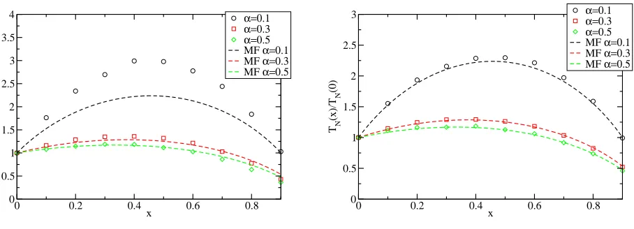
values of x can be explored. In Fig. 2 we plot the consensus time TN(α, x) computed
in lattices of dimension d = 1 and d = 2 as a function of x, and for different fixed
values of α. In order to get rid of size-dependent prefactors due to the dimensionality
in the consensus time, we normalized it by its value at x = 0, which takes the form
TN(α) =−N[αln(α) + (1−α) ln(1−α)] at mean-field level. The numerical simulations
for d = 2 fit quite precisely the theoretical mean-field prediction of the consensus time
dependence on the initial configuration~x, developed in Sec. 2, with only slight deviations
for small α and close to x ∼ 0.5. On the other hand, strong deviations are noticeable
in dimension d = 1, specially for small values of α. This result is in agreement with
the expectation for the standard voter model, in which the mean-field consensus time
0 0.2 0.4 0.6 0.8 x 0 0.5 1 1.5 2 2.5 3 3.5 4 TN (x)/T N (0) α=0.1 α=0.3 α=0.5
MF α=0.1 MF α=0.3 MF α=0.5
0 0.2 0.4 0.6 0.8
x 0 0.5 1 1.5 2 2.5 3 TN (x)/T N (0) α=0.1 α=0.3 α=0.5
[image:9.612.66.520.106.270.2]MF α=0.1 MF α=0.3 MF α=0.5
Figure 2. Normalized consensus time TN(x)/TN(0) as a function ofxfor the initial configuration~x={x, α(1−x),(1−α)(1−x)} in regular lattices of dimensiond= 1 (left) andd= 2 (right) of sizeN = 400 sites, compared with the analytical mean-field prediction Eq. (11).
3.2. Effect of the number of states
We have seen that, at the mean field level, and for homogeneous initial conditions
xi = 1/S for i = 1, . . . , S, the consensus time increases with S towards it limit value TH
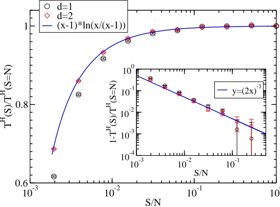
N(S =N)with a power-law form, as given by Eq. (13). In Fig. 3 we plot the rescaled
consensus time TH
N(S)/TNH(S = N) as a function of S for lattices of dimension d = 1
and d = 2 and fixed size N = 103. From this figure we observe once again that the
d = 2 behavior is well fitted by the mean-field prediction, while the d = 1 case shows
deviations for small S. Interestingly, increasing the number of initial states S reduces
the deviation from the mean-field theory, in a way that the behavior for S →N is very
well fitted by Eq. (13).
3.3. Number of surviving states s(t)
At the mean field level, the number of surviving states s(t), starting from maximally
heterogeneous conditions S = N, decays as s(t) ∼ St−β in the initial time regime,
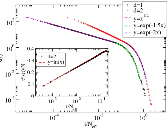
with an exponent β = 1, crossing over to a exponential decay at large times. In Fig.
4 we show the number of surviving states s(t) as a function of time corresponding to
numerical simulations on d= 1 and d= 2 lattices.
From the results of Fig. 4, it is clear that the initial decay of the density of surviving states follows, as expected, a power-law form. The decay is, however, slower than the
mean-field prediction. In particular, we see that ind= 1, s(t)∼N t−1/2, while in d= 2
numerical data can be fitted to the form s(t)∼N t−1logt, corresponding to mean-field
10-3 10-2 10-1 100 S/N
0.6 0.8 1
T
H (S)/T H (S=N)
d=1 d=2
(x-1)*ln(x/(x-1))
10-3 10-2 10-1 S/N 10-4
10-3 10-2 10-1 100
1-T
H (S)/T H (S=N)
[image:10.612.146.419.114.316.2]y=(2x)-1
Figure 3. Rescaled consensus time TH
N(S)/TNH(S = N) starting from homogenous initial conditions, as a function of the number of statesS/N in dimensiond= 1 and
d = 2, for N = 103, compared with the theoretical mean-field prediction Eq. (12). In the inset we plot the quantity 1−TH
N(S)/T H
N(S = N), showing the power-law decay withS. Error bars represent the standard deviation error on the average of the distribution. Each point is averaged over 105 runs.
particular, we find that in the large time regime we can fit s(t) ∼ exp(−1.5t/Neff) for
d= 1, while s(t)∼exp(−2t/Neff) ford= 2.
The origin of the slowing down in the decay of the number of surviving states in low dimensions can be attributed to the formation of spatial domains of sites in the same state, which have to annihilate diffusively in order to reach the consensus state. In
this line, the behavior of the number of surviving states in d= 1 can be understood by
means of a simple argument: At a given timet >1, there will be a number of surviving
states s(t). Assuming that sites with the same state form clusters, the activity will be
driven by the diffusive fluctuation of the boundaries of those clusters, which will have
a length ` ∝ t1/2. The number of different clusters will thus be s(t) ∝ N/` ∼ N t−1/2,
recovering the observed time dependence.
3.4. Effects of correlated initial configurations
Considering the multi-state voter model on a finite lattice allows to investigate the effects of correlated initial configurations in the dynamical approach to the consensus state, which should be particularly important in one-dimensional lattices. We have
thus simulated the multi-state voter model in a d = 1 lattice, stating from an initial
configuration of S states arranged in S contiguous blocks on length N/S in a lattice
10-3 10-2 10-1 t/Neff
0 0.1 0.2 0.3 0.4
t*s(t)/N
d=2 y=ln(x)
10-4 10-2 100
t/N eff 10-4
10-2 100 102
s(t)
[image:11.612.146.419.110.320.2]d=1 d=2 y=x1/2 y=exp(-1.5x) y=exp(-2x)
Figure 4. Surviving states s(t) as a function of rescaled timet/Neff for ad= 1 and d= 2 lattice ofN= 400 nodes, starting with homogeneous condition ands(0) =S=N
states. Fort Neff, the number of surviving states decays as s(t)∼t−1/2 for d= 1 and s(t)∼ t−1logt for d= 2 (inset). For large t, s(t) decays exponentially in both cases.
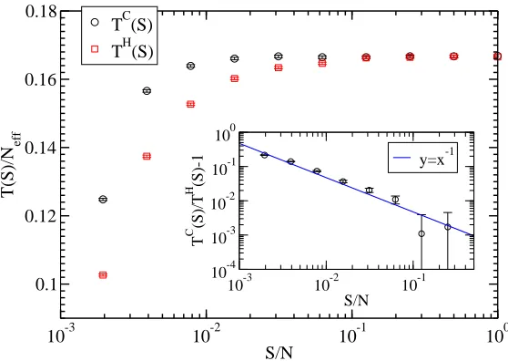
conditions as a function of S, comparing it with the consensus time starting with
uncorrelated homogeneous initial conditions, TNH(S). We find that the effect of starting
with correlated initial condition strongly slows down the achievement of consensus. As expected, the difference between the consensus time with correlated and homogeneous
initials conditions approaches zero forS →N with a behavior compatible with a
power-law form of exponent −1, i.e.
TC N(S) TN(S)
−1∼
S N −1
−1
forS→N. (20)
4. Conclusions
In this paper we have addressed the general scenario of the voter model in which the number of different states allowed in the model can be larger than two, and, in the
thermodynamic limit, even unlimited. At the mean-field level, we have presented
derivations for the expression of the exit probability, the consensus time (which generalizes naturally the ‘entropic’ form observed for the two-states case), and the
density of surviving states as a function of time. We have highlighted that in the
limit of S → ∞ the ordering time is only 1/ln 2 times bigger than in the binary voter
10-3 10-2 10-1 100 S/N
0.1 0.12 0.14 0.16 0.18
T(S)/N
eff
TC(S)
TH(S)
10-3 10-2 10-1 S/N 10-4
10-3 10-2 10-1 100
T
C (S)/T H (S)-1
[image:12.612.142.421.118.316.2]y=x-1
Figure 5. Consensus time T(S)/Neff as a function of the number of initial statesS on a d = 1 lattice withN = 103 nodes with a correlated initial configuration made of blocks of voters in the same state, of initial length N/S, TC(S), compared with the consensus time obtained with random homogeneous initial conditionsTH(S)w. In the inset we show that the quantityTc(S)/TH(S)−1 goes to zero with a power law behavior with exponent -1. Error bars are obtained as in Figure 3. Each point is averaged over 105 runs.
multi state voter model on 1− and 2−dimensional lattices, and compared the results
with the binary case. The consensus time in the d = 2 case is well predicted by the
mean-field theory, while the uni-dimensional case behaves differently. Remarkably, it increases with the number of initial states with a power-law form as predicted by the
mean-field theory, for both d = 1 and d = 2. We have also addressed the effect of
correlated initial conditions on the consensus time, finding out that the relevance of this effect decreases with the number of initial states with a power law behavior. In summary, our results show that the number of states is not a trivial parameter in the voter model, and it affects the overall dynamics in subtle ways.
Acknowledgments
References
[1] Castellano C, Fortunato S and Loreto V 2009Rev. Mod. Phys. 81 591–646
[2] Clifford P and Sudbury A 1973 Biometrika 60 581–588
[3] Holley R A and Liggett T M 1975 Annals of Probability 3 643–663
[4] Liggett T M 1999 Stochastic interacting particle systems: Contact, Voter, and
Exclusion processes (New York: Springer-Verlag)
[5] Krapivsky P, Redner S and Ben-Naim E 2010A Kinetic View of Statistical Physics
(Cambridge: Cambridge University Press)
[6] Blythe R A 2010 Journal of Physics A: Mathematical and Theoretical 43 385003
[7] Mobilia M 2003 Phys. Rev. Lett. 91 028701
[8] Mobilia M, Petersen A and Redner S 2007Journal of Statistical Mechanics: Theory
and Experiment 2007 P08029
[9] Dall’Asta L and Castellano C 2007 Europhys. Lett. 77 60005
[10] Stark H, Tessone C J and Schweitzer F 2008 Phys. Rev. Lett.101 018701
[11] Lambiotte R and Redner S 2008 Europhys. Lett. 82 18007
[12] Cox J T and Durret R 1991 Nonlinear voter models Random Walks, Brownian
Motion, and Interacting Particle Systems ed Durrett R and Kesten H (Boston: Birkhauser) pp 189–202
[13] de Oliveira M, Mendes J and Santos M 1993 J. Phys. A 26 2317–2324
[14] Wu F Y 1982 Rev. Mod. Phys.54 235–268
[15] Sire C and Majumdar S N 1995 Phys. Rev. E 52 244–254
[16] L´opez F J, Sanz G and Sobottka M 2008 Journal of Statistical Mechanics: Theory
and Experiment 2008 P05006
[17] B¨ohme G A and Gross T 2012 Phys. Rev. E 85 066117
[18] Hubbell S 2001 The Unified Neutral Theory of Biodiversity and Biogeography
Monographs in Population Biology (Princeton, NJ: Princeton University Press)
[19] McKane A J, Alonso D and Sol´e R V 2004 Theoretical Population Biology 6567 –
73
[20] Pigolotti S, Flammini A, Marsili M and Maritan A 2005 Proc. Natl. Acad. Sci.
USA 102 15747
[21] Volovik D, Mobilia M and Redner S 2009Europhy. Lett. 85 48003
[22] V´azquez F, Krapivsky P L and Redner S 2003Journal of Physics A: Mathematical
and General 36 L61
[23] Castell´o X, Egu´ıluz V M and Miguel M S 2006 New Journal of Physics 8 308
[24] Tavar´e S 1984 Theoretical Population Biology 26 119–164
[26] Baxter G J, Blythe R A and McKane A J 2007 Mathematical Biosciences 209 124–170
[27] Blythe R A and McKane A J 2007J. Stat. Mech. P07018
[28] Gardiner C W 1985 Handbook of stochastic methods 2nd ed (Berlin: Springer)