This is a repository copy of Optimal Reaction Coordinates.
White Rose Research Online URL for this paper:
http://eprints.whiterose.ac.uk/102357/
Version: Accepted Version
Article:
Banushkina, PV and Krivov, SV orcid.org/0000-0002-3493-0068 (2016) Optimal Reaction
Coordinates. Wiley Interdisciplinary Reviews: Computational Molecular Science, 6 (6). pp.
748-763. ISSN 1759-0876
https://doi.org/10.1002/wcms.1276
© 2016 John Wiley & Sons, Ltd. This is the peer reviewed version of the following article:
Banushkina, P. V. and Krivov, S. V. (2016), Optimal reaction coordinates. WIREs Comput
Mol Sci. doi: 10.1002/wcms.1276 which has been published in final form at
http://dx.doi.org/10.1002/wcms.1276. This article may be used for non-commercial
purposes in accordance with Wiley Terms and Conditions for Self-Archiving. Uploaded in
accordance with the publisher's self-archiving policy.
[email protected] https://eprints.whiterose.ac.uk/
Reuse
Unless indicated otherwise, fulltext items are protected by copyright with all rights reserved. The copyright exception in section 29 of the Copyright, Designs and Patents Act 1988 allows the making of a single copy solely for the purpose of non-commercial research or private study within the limits of fair dealing. The publisher or other rights-holder may allow further reproduction and re-use of this version - refer to the White Rose Research Online record for this item. Where records identify the publisher as the copyright holder, users can verify any specific terms of use on the publisher’s website.
Takedown
If you consider content in White Rose Research Online to be in breach of UK law, please notify us by
Optimal Reaction Coordinates
Polina V. Banushkina,
Astbury Center for Structural Molecular Biology,
Faculty of Biological Sciences, University of Leeds, Leeds LS2 9JT, United Kingdom
Sergei V. Krivov,
Astbury Center for Structural Molecular Biology,
Faculty of Biological Sciences, University of Leeds, Leeds LS2 9JT, United Kingdom,
[email protected]
July 8, 2016
Abstract
The dynamic behavior of complex systems with many degrees of freedom is often analyzed by projection onto one or a few reaction coordinates. The dynamics is then described in a simple and intuitive way as diffusion on the associated free energy profile. In order to use such a picture for a quantitative description of the dynamics one needs to select the coordinate in an optimal way so as to minimize non-Markovian effects due to the projection. For equilibrium dynamics between two boundary states (e.g., a reaction) the optimal coordinate is known as the committor or the pfold coordinate in protein folding studies. While the dynamics projected on the committor is not Markovian, many important quantities of the original multidimensional dynamics on an arbitrarily complex landscape can be computed exactly. Here we summarize the derivation of this result, discuss different approaches to determine and validate the committor coordinate and present three illustrative applications: protein folding, the game of chess, and patient recovery dynamics after kidney transplant.
Introduction
A popular approach to analyze complex multidimensional dynamics is to project it onto a reaction co-ordinate (collective variable) that captures the essential properties of the dynamics. For simple chemical reactions the choice of coordinate is often self-evident, e.g., an inter-atomic distance. The reaction is then described as diffusion on a free energy profile (FEP) as a function of the coordinate, with the dynamics of the rest of the degrees of freedom modeled as noise. Such a picture provides a simple and intuitive description of the dynamics. Selection of reaction coordinates for complex reactions, e.g., protein folding, is far from trivial, especially if one requires a quantitative description of the dynamics. A poorly chosen coordinate can result in a misleadingly simple free energy landscape1 with lower barriers and incorrect, faster kinetics2 and generally sub-diffusive dynamics.3–5 In principle, dynamics projected on any coordi-nate can be accurately described by the generalized Langevin equation, which contains a memory kernel that accounts for non-Markovian effects.6,7 Determination of the kernel is, however, very difficult.8 More-over, it complicates the conceptually simple and visually appealing picture of reaction as simple diffusion on a free energy landscape. Under some conditions (e.g., the separation of time scales) the generalized Langevin equation can be reduced to the standard memory-less Langevin equation. Often, however, such conditions are very restrictive, and it is not clear how to test their validity for a practical system of interest (e.g., barrier-less or fast protein folding).
quantities can be computed exactly for the original dynamics on a multidimensional free energy landscape of any complexity. For equilibrium dynamics between two boundary states (e.g. unfolded and folded), such an optimal coordinate is known as the committor, splitting probability orpf oldcoordinate for protein
folding studies.
The paper is organized as follows. We start by reviewing why the committor can be considered as an optimal reaction coordinate (RC). Then we consider different approaches to determine and validate the optimal RC in practice, which is followed by a brief comparison with other popular dimensionality reduction techniques. The next section presents illustrative examples. We conclude by suggesting unsolved problems and directions for future research. This review is complementary to two excellent recent reviews on reaction coordinates.10,11
The committor as an optimal reaction coordinate.
In a description of reaction dynamics the following quantities are of particular interest: the reaction flux, the mean first passage times, the mean transition path times. While, in principle, one may expect a different optimal coordinate for each of the quantities, the committor can be used to compute all of them exactly.
The committor equals the probability for the trajectory to reach one boundary state (e.g., the native state in the analysis of protein folding) before it reaches another (e.g., the denatured state) starting from any given configuration. It was first used for the analysis of ion recombination dynamics by Onsager.12 In the protein folding field it was first used by Duet al.13 Its role in the statistics of transition paths has been investigated in a number of studies.14,15 More details about historical developments can be found in a recent review.10
For equilibrium dynamics (with detailed balance) described by the overdamped Langevin equation the associated Fokker-Planck (diffusion) equation for probability density function is
∂P(X, t)/∂t=∇ ·[e−βU(X)D(
X)∇(eβU(X)P(
X, t))], (1)
whereX denotes position in the multidimensional configuration space,U(X) is the potential energy,D
is the diffusion tensor,β = 1/(kT) and k is the Boltzmann constant and T is temperature. Given two boundary states A and B, the committor is the solution of the adjoint equation16,17
∇ ·[e−βU(X)D(
X)∇q(X)] = 0, q(X ∈∂A) = 0, q(X∈∂B) = 1. (2)
For equilibrium dynamics described by a Markov chain
Pi(t+ ∆t) =
∑
j
Pij(∆t)Pj(t), (3)
wherePi(t) is the probability of being in stateiat timetandPij(∆t) is the probability of transition from
statej toi after time interval ∆t, the committor functionqi is defined as the solution of
qi=
∑
j
Pji(∆t)qj, qA= 0, qB = 1. (4)
Eq. 4 rewritten as
∑
j
Pji(∆t)(qj−qi) = 0 (5)
illustrates the driftless character of dynamics projected on the committor coordinate: the average dis-placement from any state (but the boundary states) is zero.
between any two boundary states A and B, as well as between any two associated isocommittor surfaces
q(X) =q0andq(X) =q1. Also, the equilibrium mean squared displacement grows linearly with time as for simple diffusion.9,19 Consequently, F(q) andD(q) can be used to define the free energy barrier and pre-exponential factor - other major descriptors of reaction dynamics.
Below we briefly summarize the derivation of these results following the formalism of Ref. 9 and highlighting points in common with those of Refs. 17 and 16. The former utilizes the Markov chains while the latter use the Fokker-Planck equation. We prefer the formalism of Markov chains because it makes some facts easier to express and to prove (e.g., compare Eq. 4 and 2) and operates with quantities computable directly from a trajectory, and thus can be straightforwardly tested and used in practice. Since a Markov chain can be considered as a discrete approximation in solving the Fokker-Plank equation both descriptions can be used interchangeably.
Given a long equilibrium trajectory X(i∆t0) and RC R(X), the RC time series is computed as
r(i∆t0) =R(X(i∆t0))). Here and belowrdenotes an arbitrary RC whileqis reserved for the committor; ∆t0 denotes the time step of the trajectory. The conventional (histogram) free energy profile is computed as
FH(r) =−kTlnZH(r), ZH(r) =Nr/∆r (6)
andNris the number of trajectory points in histogram bin with boundariesrandr+∆r. ZHapproximates
(up to a factor) the partition function
Z(r) = ∫
exp[−U(X)/kT]δ(r−R(X))dX.
In particular, the equilibrium probability is Peq(r) = ZH(r)/N = Z(r)/Z, where N denotes the total
number of points in the trajectory and Z = ∫
Z(r)dr is the total partition function. A very useful quantity is the partition function of a cut free energy profileZC,1.9 It equals half the total distance the
system moves when it transits through the pointr, namely
ZC,1(r,∆t) = 1/2∑ri|r(∆t+i∆t)−r(i∆t)| (7)
where ∑r
i denotes the sum only over such i when r is between r(∆t+i∆t) and r(i∆t). This quantity
can be computed by considering every time step (∆t = ∆t0) of the trajectory, every second time step (∆t= 2∆t0), third and so forth, which is indicated by the dependence on ∆t. If the original dynamics in the configuration space is Markovian and equilibrium and the reaction coordinate equals the committor between any two boundary regions A and B, thenZC,1is constant with respect toqand ∆t.9It corresponds to constants J in Ref. 17 (Eq. 2.6) and ν in Ref. 16 (Eq. 18). The constancy of ZC,1 follows from the driftless character of projected dynamics (Eq. 5). Since it is violated at the boundaries, a special counting method using the ensemble of transition path segments is employed for ∆t >∆t0,9which restores driftlessness at boundaries and makes ZC,1 constant everywhere. Another option is to combine the RC and its mirror image into a ring and thus eliminate boundaries.19,20The constant value ofZ
C,1computed for very large ∆tequals the total number of transitions the trajectory makes from one boundary node to the other9
ZC,1(q,∆t) =NAB. (8)
In the opposite limit of very small ∆t, whenZH(r) can be considered constant on the range of average
dis-placementr(t+ ∆t)−r(t), by direct computation from Eq. 7 one obtainsZC,1(r,∆t) = 1/2⟨∆r2⟩ZH(r) = D(r)∆tZH(r), which can be used to determine the position dependent diffusion coefficient along any RC9
and specifically for the committor coordinate
D(q) = NAB ∆tZH(q)
. (9)
Such determinedF(q) (Eq. 6) andD(q) (Eq. 9) define a diffusive model for the dynamics projected on the committor. The corresponding Fokker-Plank equation is obtained by substitutingF(q) and D(q) into one-dimensional Eq. 1
∂P(q, t)
∂t =JAB
∂2
∂q2(
P(q, t)
Peq(q)
).
It was first derived by Berezhkovskii and Szabo.17For the model one has identicallyN
AB = ∆tZH(q)D(q).
The number of transition between the boundary states per unit timeJAB =NAB/(N∆t0), the
equilib-rium flux, equalsJAB−1 = (ZH(q)D(q)/N)−1=∫01e−F(q)/kTdq∫01e−F(q)dq/kTD(q). Since both integrands are reparametrization invariant one obtains the following Kramers-like equation
J−1
AB =
∫ q′(B)
q′(A)
e−F′(q′)/kT dq′∫
q′(B)
q′(A)
dq′
e−F′(q′)/kTD′(q′), (10)
whereF′ andD′ are functions of an arbitrary RCq′ related to the committor by a monotonous
transfor-mation. A practically convenient choice is a coordinate with constant diffusion coefficientD′ = 1. In this
case one has to visualize just the free energy profile which completely describes the diffusive dynamics. The mean first passage time from A to B (here we assume that time spent in A is negligible or that equilibration in A is fast) equals14
mfpt = 1/JAB
∫ 1
0
Peq(q)(1−q)dq=<1−q > /JAB, (11)
and thus can be computed exactly since we can compute exactlyPeq(q),qandJAB. The same is true for
the mean transition path times between A and B, which can be computed as14
mtpt = 1/JAB
∫ 1
0
Peq(q)q(1−q)dq =< q(1−q)> /JAB. (12)
Integrating Eq. 7 over r one obtains19,22
∫ 1
0
ZC,1(r,∆t)dr= 1/2
∑
i
[r(∆t+i∆t)−r(i∆t)]2= 1/2⟨∆r2(∆t)⟩(N∆t0)/∆t
or
⟨∆r2(∆t)⟩= 2∆t/(N∆t0)⟨ZC,1(∆t)⟩, (13)
which means that if⟨ZC,1(∆t)⟩is constant (increases with ∆t, decreases with ∆t) the equilibrium mean
squared displacement grows linearly (faster than linear, slower than linear) with time.9For the committor one specifically obtains⟨∆q2(∆t)⟩= 2∆tJ
AB. This suggests that one of the reasons that the dynamics of
various protein degrees of freedom is sub-diffusive3–5is because these degrees are not optimal RCs.9Note that, for large ∆tthe averaging should use the transition path segments, so that boundary effects do not change the diffusive behavior.9
Equation q(X) = q∗ defines the isocommittor surface, which consists of all the configurations that
have the same value of the committor (q∗). Such a surface partitions the configuration state on two parts
and asq∗ changes from 0 to 1 the surface monotonously progresses from state A to state B. The surface
corresponding toq∗= 0.5 is known as the stochastic separatrix and is often used to define the ensemble
of the transition states. Ref. 23 presents illustrative examples of isocommittor surfaces for a number of model systems. Two isocommittor surfaces corresponding toq0andq1, withq0< q1, can be used to define two new boundary states A′: q(X)< q
0 and B′: q(X)> q1. The committor function between these new boundary states can be obtained by simple rescalingq′(X) = (q(X)−q0)/(q
1−q0).16 The above results are therefor valid not just for two boundary points on the committor (i.e.,q0=0 and q1=1) but between any two pointsq0andq1.
constant but different diffusion coefficientsD1 and D2. The committor coordinate equalsx. Markovian behavior means that the future dynamics depends only on the current state of the system and not on previous states, e.g., that there is no correlation between the current and next displacements, in particular that⟨[q(0)−q(−∆t)]2[q(∆t)−q(0)]2⟩=⟨[q(0)−q(−∆t)]2⟩⟨[q(∆t)−q(0)]2⟩. However, as one can easily show in this case, these quantities are 2(D2
1+D22)∆t2 and (D1+D2)2∆t2, respectively.
We conclude this section by noting that while the committor is often considered synonymous with the optimal coordinate, it is an optimal coordinate only for the specific, though important, case of equilibrium dynamics between two boundary states (i.e., a reaction). Here the general driftless character of dynamics projected on the optimal coordinate is combined with specific boundary conditions (Eq. 4) which allows interpretation of the coordinate as the committor. Consider diffusion on a ring, e.g., a model for dynamics of a molecular motor or for a dihedral angle of alanine dipeptide.2An optimal coordinate for such dynamics has no boundaries and is a multi-valued function (similar to the angle variable) with dynamics driftless everywhere.19 It can not be interpreted as a committor. However its analysis using cut profiles becomes less involved, since one does not need to consider the ensemble of transition path segments.19,20
Validation and determination of optimal RCs
If one intends to use an RC for quantitative analysis of dynamics it is important to validate and demon-strate that this RC is optimal, especially, if this RC was determined by a generic dimensionality reduction method rather than a method explicitly focused on determining the optimal RC. Since a criterion for RC optimality can be often turned into an optimization method, we review them together.
We start with the simplest conceptually - the direct method to determine the committor, where one starts a number of trajectories (usually around 100) from the point of interest and computes their evolution until they reach either of the boundary states.13,24–27The committor is estimated as the fraction of trajectories that reached state B. A genetic neural network (GNN) method can utilize such obtained committor values to identify the combination of coordinates that produces the most accurate prediction of the committor.26 To reduce the computational costs of evaluating the committor for every point of a reactive trajectory Li and Ma have suggested to model time evolution of committor using a sigmod function.27
The committor histogram test is a direct method to test the optimality of an RC.13,24,25 If a puta-tive reaction coordinate r(X) closely approximates the committor, then an ensemble of configurations corresponding tor(X) =r0should have similar committor values. Ideally, the distribution of committor values should beδ-picked aroundq(r0). In particular, for the transition state ensemble of configurations, the distribution should be narrowly picked around 1/2. Deviations from the ideal shape indicate that the putative RC does not include some important degrees of freedom (y) and can be also used to infer a qual-itative picture of the free energy landscape as a function of the coordinatesF(r, y).24,25 The committor for each of the configurations is determined by the direct method. Peters has suggested how to reduce the computational cost by using binomial deconvolution.28
For relatively small systems, where an accurate Markov state model (MSM) can be constructed,2,29,30 the committor coordinate between any two states can be easily found by solving Eq. 4. Which, incidentally, suggests a way to validate an MSM by validating the determined committor.9
For large systems the determination of accurate MSMs (specifically at transiently populated TS re-gions) is difficult.9,30,31 For such systems a number of variational approaches have been suggested to determine the coordinate, without explicitly constructing the MSM. To this end, a functional form for the RC containing many parameters is suggested. For example, for protein folding, one can take a weighted sum of native and non-native contacts ∑
ijwijqij,32 a sum of contacts with varying cutoff distances
∑
ij±θ(rij−r0ij),3,33,34a weighted sum of interatom distances
∑
ijwijrij,3 or more complex functions.21
Then, one numerically optimizes the weightswij32or the cutoff distancesr0ij3,33,34for contacts by
optimiz-ing a particular functional, so that in the end, the putative reaction coordinate accurately approximates the committor. The following optimization functionals have been suggested: the probability of being on a transition path,32,35 the likelihood functional,36,37 the cut profiles,3,33,34,38 and the total squared displacement (TSD).22,39
the optimal coordinate using transition path segments is constant and equal toNAB.9 In particular, it
implies that the computed reaction flux is exact, the equilibrium mean squared displacement grows linearly with time, etc. IfZC,1(r,∆t) decreases with increasing ∆tor, correspondingly,FC,1(r,∆t) increases, then
consecutive displacements are negatively correlated and the dynamics is sub-diffusive.9 On the contrary,
ZC,1(r,∆t) increasing with ∆t is an indication of overfitting. The latter, in particular, can be used
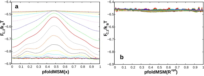
to penalize overfitting during RC optimization.9,33,34 Fig. 1 illustrates the criterion on the extensively sampled model system with two parallel one-dimensional pathways, where now D1 = D2 = 0.0001,
F1(x) = 2 exp[−9(3x−1)2],F2(x) = 2 exp[−9(3x−2)2] andxis not the optimal RC.22
−6.9 −6.8 −6.7 −6.6 −6.5 −6.4
0 0.1 0.2 0.3 0.4 0.5 0.6 0.7 0.8 0.9 1
F /k TC,1
pfoldMSM(x)
B
a
−6.9 −6.8 −6.7 −6.6 −6.5 −6.4
0 0.1 0.2 0.3 0.4 0.5 0.6 0.7 0.8 0.9 1
F /k TC,1
pfoldMSM(R )
B
[image:7.612.107.503.176.325.2]opt
b
Figure 1: FC,1criterion applied to a model system. (a)FC,1increases with increasing ∆tindicating thatx coordinate is sub-optimal. (b)FC,1is approximately constant, indicating that the putative coordinateRopt closely approximates the committor. The plots were prepared with the fep1d.py script.40. Reproduced with permission from Ref.22
The criterion suggests a general optimization idea - to minimizeZC,1(r) or maximize FC,1(r).
Min-imization of ZC,1(r) makes dynamics less sub-diffusive and thus more Markovian. One option is to
maximize∫rB
rA dr/ZC,1(r), where rA andrB denote positions of free energy minima alongr.
34 Since the
main contribution to this functional comes from points with lowZC,1(r), the optimization is focused on
the transition state regions. An additional bonus is that this functional is invariant to monotonous trans-formations of RC, which simplifies the task of approximating the committor.33,34 A different functional with analogous properties, which was used originally, is ∫rB
rA ZH(r)dr/ZC(r).
3,33,38 Another option is to
minimize∫rB
rA ZC,1(r)dr= 1/2 ∑
k[r(∆t+k∆t)−r(k∆t)]2, i.e., the TSD under constraintsrA = 0 and rB = 1.9,22,39The fact that the minimum of the TSD is attained for the committor can be easily verified
using the following expression for the TSD for an MSM∑
ijnij(ri−rj)2, wherenij =nji=Pij(∆t)Peq,jis
the equilibrium number of transitions between statesiandj.22 Differentiating the TSD byr
k and
equat-ing to zero one obtains Eq. 4. The main contribution to the TSD functional comes from the points with highZC,1(r), i.e., the optimization is focused on free energy minima. An advantage of such a functional
is that its optimum can be found analytically when the RC is a weighted sum of basis functions.22,39This feature lead to a new method which optimizes the RC over the entire range, not just around the transition state regions.22 From Eq. 13 it follows that the TSD of the committor equals 2N
AB, i.e., one obtains a
simpler though less stringent optimality criterion.22
An advantage of the approach of using cut profiles ZC,1 is that a single framework is used to derive theoretical results, to determine and validate optimal coordinates and to determine the diffusion coefficient. Another advantage is that the approach can be straightforwardly extended to optimal RCs with a ring topology.
optimality. It follows that ZC,1(q(r)) = const. If the flux is reproduced then NAB = ZC,1(q(r)) =
1/2∑
k[q(r(∆t+k∆t))−q(r(k∆t))]2. The TSD attains its minimum value of 2NAB only when the RC q(r(X)) is optimal (we assume there is no overfitting), which means thatris optimal.22
Bayesian criterion p(TP|q). A Bayesian criterion quantifies the quality of an RC by calculating the probabilityp(T P|r) of being on the transition path (TP)32,35
p(T P|X) =p(X|T P)p(T P)/peq(X),
where p(X|T P) is the probability density of X on the TP, p(T P) is the fraction of time spent on the TP, and peq(X) is the equilibrium probability density at point X of configuration space. For diffusive
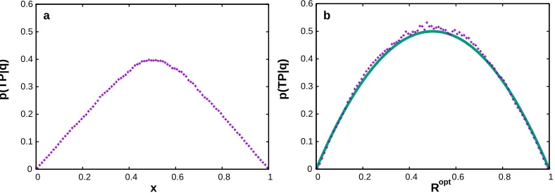
dynamics p(T P|X) = 2q(X)(1−q(X)), which reaches its maximum of 0.5 exactly at the points of the stochastic separatrixq(X) = 0.5.35For a good reaction coordinater=R(X),p(T P|r) should have a single sharp and high peak, collapsing the transition states with a high value ofp(T P|X) into a single value ofq.32 The stochastic separatrix, is a reasonable definition of the transition state ensemble for systems with one dominant barrier. However caution should be used for systems with more complex landscapes. For example, in a system with two approximately equal barriers,33q(X) = 0.5 describes an intermediate state, rather than the transition states. Fig. 2 illustrates the criterion on the model system with two pathways.22
0 0
0.1 0.1
0.2 0.2
0.3 0.3
0.4 0.4
0.5 0.5
0.6 0.6
0
0 0.2 0.4 0.6 0.8 1 0.2 0.4 0.6 0.8 1
p(TP|q)
p(TP|q)
R
x opt
[image:8.612.110.504.289.426.2]a b
Figure 2: p(T P|q) criterion applied to a model system (symbols) using a sub-optimal coordinate (a) and putative optimal coordinate (b). The line shows the theoretical maximum of 2q(1−q). The plots were prepared using the fep1d.py script.40
It is straightforward to turn the Bayesian criterion into an optimization method: one optimizes the parameters of a putative reaction coordinater to make p(T P|r) maximal.32 Once the optimal RC has been determined, the associated free energy profile and diffusion coefficient are determined using a different Bayesian procedure.43
Likelihood maximization. The maximum likelihood method can be used to screen reaction coor-dinates based on an ensemble of trajectories generated by an aimless shooting variant of transition path sampling (TPS).36 The likelihood for optimizing a model of the committor ˜qis
L=∏
k
˜
q(Xk)
∏
k′
(1−q˜(Xk′)),
wherekandk′ denote trajectories that reached states B and A, respectively. Inspired by the exact result
for a parabolic barrier, the following model is used ˜q(X) = 1/2 erfc[−(r(X)−r†)/∆r], where r(X) is
the putative reaction coordinate, r† is the transition state location and ∆r is the width of the barrier.
Parametersr† and ∆rare optimized together with the parameters of RC, which the RC being taken as a
linear combination of various collective variables. The optimization stops when the Bayesian Information criterion identifies the point of diminishing return. The inertial likelihood maximization method37which is more accurate in the regime of inertial barrier crossing dynamics employs the following model for the committor: ˜q(X) = 1/2 erfc[−(r(X)−r†)/∆r+br˙], where ˙r= ˙X∇rdenotes the velocity along the putative
the TPS may become inefficient, one may study each barrier separately.44,45 The likelihood methods are discussed in more detail in two recent reviews.11,46 While the likelihood function can be used to compare two putative RCs there is no straightforward way to use it as a validation criterion. One drawback of using a TPS ensemble of trajectories for training an RC is that such an optimized RC is not likely to be transferable for analysis of trajectories from equilibrium simulations which sample the entire configuration space.
Dynamical self-consistency test. This test inspects whether averaging during projection on a putative reaction coordinate does not change the dynamics, or in other words that similar dynamics are combined. Specifically, the dynamics of short trajectories launched from an ensemble of configurations (Xi) on isosurfaces of a trial coordinater(Xi) =r0are projected back onto the trial coordinate to estimate numerically the propagatorPi(r, t|Xi). The trial coordinate has a dynamically self-consistent projection
property if the dynamics of individual swarms at each point evolve like swarms initiated from all other points on the same trial coordinate isosurfacePi(r, t|Xi)∼P(r, t|r0), whereP(r, t|r0) =⟨Pi(r, t|Xi)⟩i.47
The propagators are compared by computing the Kullback-Leibler divergence between the distributions. Note that while intuitively appealing, this criterion is probably as stringent as the requirement of projected dynamics to be Markovian. For example, it is violated by the committor coordinate for the model system with two parallel pathways described in the previous section.
Approximation of the committor by eigenvectors. Berezhkovskii and Szabo have shown that for a system with two states and a large free energy barrier, the committor can be approximated around the transition state by a second left eigenvector.48This can be determined by a number of approaches currently under active development.22,30,31 Such eigenvectors, in particular, can be useful as seed coordinates to start RC optimization, especially in cases where the boundary states are not straightforward to define.22 In summary, a number of practically efficient tests for validation of optimal RCs have been devel-oped. Some of them (ZC,1 = const and p(T P|q)) have been implemented in the fep1d script http: //sourceforge.net/projects/fep1d/developed for the analysis of one-dimensional reaction coordinates and the resulting dynamics along them.40 However, the development of efficient and robust methods to determine the committor for complex realistic systems which can pass the validation tests is still mostly work in progress.
Other dimensionality reduction techniques.
It is instructive to compare methods that seek optimal RCs with other popular dimensionality reduction techniques. The techniques can be divided roughly into two groups: techniques that use dynamical information during dimensionality reduction and those that do not. Coordinates obtained with the former are likely to reproduce the dynamics more accurately than those obtained with the latter. The latter group, in particular, includes all the methods, where results do not change if points in a trajectory are reshuffled, e.g., PCA and its various modifications,49multidimensional scaling,50 Laplacian eigenmaps,51 locally linear embedding,52Isomap,53 and Sketchmap.54
Some methods aim at obtaining accurate Markov models of the dynamics in the projected space. This is a stronger result than is guaranteed with optimal coordinates. In particular, it means that all quantities of the projected dynamics could be computed exactly. The methods usually assume either a separation of times scales or the existence of a low-dimensional manifold to which the dynamics is confined after some initial lag time.55In practice, at least in atomistic simulations of protein folding, it is not straightforward to test the validity of these assumptions.
Interestingly, the related method of diffusion maps designates the eigenfunctions of the backward Fokker-Planck operator as optimal coordinates.58 They are optimal in a different sense compared to the committor. They provide the best approximation to the probability distribution in the formP(x, t|x0) = ∑
jαj(x0)vj(x) in a specific diffusion distance metric.58
Illustrative examples
The examples below have been chosen to illustrate the broad applicability of the framework of optimal coordinates. They show that the free energy as a function of the optimal RC provides a simple, visually appealing picture of complex dynamics and can be used to accurately determine some quantities of interest.
Protein folding.
In spite of many decades of studying how proteins fold, widely differing opinions exist even for the funda-mental issues and interpretation of many folding experiments.59 One can argue that we have determined few (if any) quantitatively accurate protein folding free energy landscapes. In particular, there is no direct estimation of the folding free energy barrier or the pre-exponential factor. Direct determination of these quantities from experiment has been hampered by very limited spatial and temporal resolution even with state of the art techniques. The situation has significantly improved recently, e.g., one can now directly estimate the transition path times during folding events by counting single photons.60,61 However, inter-pretation of the experiment still assumes a particular shape of the folding free energy landscape, which can not be established in a direct manner.
Atomistic simulations have practically unlimited spatial and temporal resolution and thus, in principle, should allow one to determine these quantities in a rigorous and direct manner. One should just take a protein, simulate its folding-unfolding dynamics for a sufficiently long time (hundreds of events), deter-mine the optimal reaction coordinate (herepf old), validate it by the optimality criteria and compute the
associated free energy profileF(pf old) with diffusion coefficientD(pf old). There are, naturally, challenges
associated with this approach: the accuracy of force-fields, sampling problems, and rigorous analysis.62 However, the steady development of theory, analysis and simulation algorithms and hardware make this approach very promising. In particular, Shaw and coworkers, using the custom build supercomputer An-ton, have been able to perform direct (brute-force) equilibrium folding simulations of 12 proteins.63This means that the force fields are already good enough to fold some of the proteins to their native structures. Note that reasonably small errors in force-fields can be tolerated if one is interested in generic properties of protein folding free energy landscapes. Below we show application of optimal RCs to the analysis of equilibrium simulations of proteins FIP35 and HP35, obtained by Shaw and coworkers.21,64
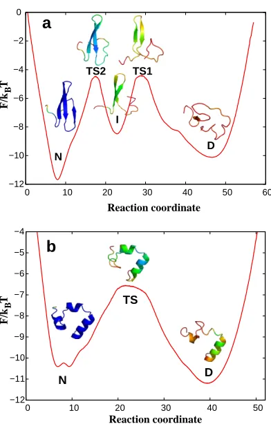
Fig. 3a shows the free energy as a function of the optimal coordinate for a FIP35 folding simulation.33 The 200µs trajectory contains 15 folding-unfolding events.21The complex landscape suggests that FIP35 is not an incipient downhill folder, it folds via a populated on-pathway intermediate separated by high free energy barriers; the high free energy barriers rather than landscape roughness are a major determinant of the rates for conformational transitions; the pre-exponential factor for the first transition state (TS1) isk−1 0 ∼10 ns. Direct detailed comparison of the pre-exponential factor with the experimental estimate of∼1
µs is complicated by the presence of the intermediate state which can not (yet) be detected experimentally. In particular, an alternative interpretation suggests to describe both the intermediate state and barriers as a single broad smooth transitions state with some roughness taken into account by an ”effective” diffusion coefficient.21,65 Multiple free energy barriers on a free energy landscape (roughness) can be described by an effective diffusion coefficient when ”many fluctuations in roughness take place in the distance of interest“.66 Whether such a description is preferable for the system with just two barriers is not clear.
In this respect the HP35 Nle/Nle double mutant (Fig 3b) is a better alternative.67 The trajectory contains many more folding-unfolding events (160) due to faster folding rate and longer length of trajectory. The profile has a single major transition state with a high broad free energy barrier. The pre-exponential factor for this barrier, estimated by four different methods, is in the range of 18 - 63 ns.
−12 −12
−11 −10
−10 −8
−9 −6
−8 −4
−7 −2
−6 0
−5 0
D TS2
I
b
a
N
−4
10
0
20
10
30
20
40
30
50
40
60
50
F/k T
F/k T
Reaction coordinate Reaction coordinate
B
B
N
TS
[image:11.612.207.403.194.501.2]D TS1
may contain additional unresolved complexity, i.e., sub-minima separated by small barriers. The mfpt determined from the profile by using Kramers equation is about 2 times shorter than that determined directly from trajectories, which means that the coordinate is close topf old but not yet equal to it.
More applications of optimal RCs to the analysis of atomistic simulations of biomolecules can be found elsewhere.3,21,32,44,63,68,69Applications to the analysis of atomistic simulations of crystallization have been reviewed in Refs. 11,46.
As mentioned above, obtaining long equilibrium trajectories for systems with complex landscapes (e.g., protein folding, large conformation changes in biomolecules) is a very difficult problem. A number of ap-proaches have been suggested to overcome the sampling problem, for a recent review see Ref. 70. Among the most popular approaches are the transition path sampling71, umbrella sampling72 and metadynam-ics73. Here we briefly touch upon the subject of how such approaches can be used to optimize RCs. The maximum likelihood approach has been suggested to optimize RCs based on transition path sampling trajectories, as described above. Umbrella sampling and metadynamics improve sampling by biasing it along collective variables. While it is relatively straightforward to recover equilibrium properties from biased simulations, the determination of dynamics properties is much more difficult. Using the biased simulations to optimize RCs is correspondingly difficult. One possibility is to use such an obtained equi-librium ensemble as starting configurations to run short unbiased MD trajectories, which then are used to optimize RC. It was used in the spectral gap optimization approach.74The optimized RC can then be used, in turn, to bias sampling, suggesting an iterative scheme. A general problem associated with biased sampling is how to ensure and validate that the biased sampling has covered all the important parts of configuration space of the original unbiased ensemble. If most of the reactive trajectories are concentrated in a narrow tube, one can use the finite temperature string method.75 Its application to conformational transitions in myosin is presented in Ref.76.
The game of chess.
Analysis of the game of chess38is interesting for several reasons. It is a model for human decision-making. Its complex dynamics is not generated by a physical system (e.g., Eqs. 1 and 3) and thus the applicability of the free-energy landscape framework is not evident. Additional complexity comes from the dynamics being inherently non-equilibrium, i.e., the games proceed from the starting position to a checkmate and never backward.
A chess program value function was used as a functional form for the RC. It gives a quantitative estimation of the value of a position as a weighted sum of various factors, with the largest factor being the difference in material. For example, a pawn has a material value of 100 and a queen of 1100. The dynamics projected on the value function with parameters used in the chess program was found to be sub-diffusive, i.e., an indication of a sub-optimal reaction coordinate. The coordinate was optimized using an ensemble of 10000 games, ending in a victory of black or white, played by the computer against itself. The equilibrium free energy profile was obtained by re-equilibrating the projected dynamics, assuming diffusive motion or using a MSM.
Fig. 4a shows the free energy as a function of the optimal RC. The game of chess is described as diffusion on the free-energy profile. Starting from the middle, the game continues until either the right (white wins) or the left (black wins) end of the profile has been reached. A lower barrier for white indicates that white has more chances to win: 59% of analyzed games ended in white’s victory. While the starting position is symmetric, white has the inherent advantage of the first move. Fig. 4b shows that the winning probability (for white) for a given position computed using three different approaches are in excellent agreement.
Knowing the winning probability (the committor) suggests an easy strategy to play chess: select a move that (after the best answer by the opponent) has the largest committor. In fact, there are many similarities between the artificial intelligence research on board games and finding an optimal RC, which suggests that mutual exchange of state of the art ideas could be useful. With that in mind we summarize below an important recent progress.
rmblkans opopopop 0Z0Z0Z0Z Z0Z0Z0Z0 0Z0Z0Z0Z Z0Z0Z0Z0 POPOPOPO SNAQJBMR
0Z0Z0Z0Z Z0Z0Z0Z0 0Z0Z0Z0Z Z0Z0Z0Z0 0Z0Z0Z0Z Z0Z0ZkZ0 0Z0Z0ZqZ Z0Z0Z0ZK
0Z0Z0Z0Z S0Z0Z0Z0 0Z0Z0Z0Z Z0Z0Z0Z0 0Z0Z0Z0Z j0J0Z0Z0 0Z0Z0Z0Z Z0Z0Z0Z0
0.01
0 −6
0.2 −5
0.4 −4
0.6 −3
0.8 −2
0.1 1
−1
−20 0
−10 1
0 10 20
1
−12
Probability to win
black wins white wins
F/kT
−8 −4 0
X
b
a
[image:13.612.208.404.210.496.2]final positions, analogous to computing the committor from an MSM. For games where an exhaustive search is impossible, one tries to approximate ν(s). For the chess game a good approximation can be found with relative ease (e.g., the major contributing factor is the material value). For the game of Go, it is much more difficult since the effect of putting a stone could be seen only much later in the game. Combined with the much larger search space, this explains why a computer program has defeated the best human player in Go just very recently, while for chess that happened almost 20 years ago. The progress is due to mainly two ideas.77The first idea is to use Monte Carlo approaches to estimateν(s) by playing a number of games from the current position. It is analogous to the direct way of estimating the committor. Second, is to approximate the value function by using deep convolutional neural networks instead of a linear combination of input features. The associated techniques could be very useful for the determination of optimal RCs.
Disease dynamics.
The evolution of disease or the progress of recovery of a patient is a complex process, which depends on many factors. A quantitative description of such a process in real-time by a single, clinically measurable parameter (biomarker) would be helpful for early, informed and targeted treatment. Conventionally, a biomarker is sought by finding a difference between two cohorts of patients, the one with the disease and a control. While undoubtedly useful, such biomarkers provide too coarse-grained a description: a patient is either healthy or has the disease, e.g., similar to order parameters with similar shortcomings. If something starts to go wrong, one may need to wait a long time to be certain about the onset of disease: until the change of a biomarker is sufficiently large, or a biomarker is well inside the abnormal state.
Considering disease dynamics as a Markovian process in the configuration state of an organism (i.e., the genome, proteome, metabolome, epigenome, age, environment, and whatever additional information may be required) it is natural to find an optimal coordinate that provides a description of the transition dynamics between two boundary states: healthy and abnormal. Interestingly, the optimal coordinate in this case - the likelihood of a positive outcome can be considered as an ideal biomarker. It can be used for monitoring purposes and maximization of such a function can serve as a basic guiding principle of targeted therapeutic intervention.
The possibility of using the framework of optimal RCs to determine such biomarkers has been demon-strated recently by analyzing the recovery dynamics after kidney transplant.39 Based on NMR spectra of blood from 18 patients, taken immediately before and in a week-long period after kidney transplant, an optimal biomarker was determined in an unsupervised way, which allows one to predict the likelihood of transplant organ success or failure earlier than with standard invasive methods (Fig. 5). The clinical group to which each patient could be ascribed is apparent from about the second day after surgery. The likelihood of a positive outcome estimated directly from patient trajectories and by describing the disease dynamics as diffusion on the free energy profile are in very good agreement.
The functional form of the RC was taken as x = ∑
jαjIj, where Ij is the intensity of the NMR
signal in bin j logarithmically transformed as Ij = log(106Ij+ 1). While the cohort contained only 18
patients, the robustness of the analysis was demonstrated by repeating it with different transformations (e.g., Ij = √Ij) or without transformation, with different bin sizes, in a supervised or unsupervised
1 2 3 4 5 6 7 8 9 10 11 12 13 14 16 17 18 21
−1
−2 0 1 2
0.0 0.4 0.6 0.8 1.0
0.2
P
1
0
−1
−2
−3
X F
t (days)
1
2
3
4
5
6
7 0
a
b
Figure 5: a) Time evolution of kidney transplant patient trajectories projected on the optimal biomarkerx
[image:15.612.210.406.175.521.2]Conclusion.
Optimal reaction coordinates can be used to provide simple and intuitive while quantitatively accurate pictures of complex dynamics as diffusion on a free energy landscape. While systematic research into optimal RCs has started only recently,10 this review demonstrates significant progress in theory and method development as well as a broad range of applications. Below we list some questions, which we believe, deserve to be attacked next.
While one may conclude that a number of practically efficient criteria to validate RC optimality have been developed, the same can not be said about methods to determine the optimal RC. There is a major practical need for efficient and robust methods to determine the committor and associated free energy profile and diffusion coefficient with high accuracy as validated by the optimality criteria. In particular, these methods are required for the analysis of state of the art atomistic simulations63 and other types of Big Data (e.g., whole brain neural recordings78) which are becoming increasingly available. A related question is how to select an appropriate functional form for a putative RC.11 It should provide a good approximation to the committor using a relatively small number of parameters. The complexity of the task becomes apparent if one recalls that the function should be able to accurately project a few million snapshots from a very high dimensional space. It is likely that the best functional forms will be system specific. However, it could also be useful to borrow from the vast experience in multidimensional function approximation of the machine learning31,77 and quantum physics79 communities. An alternative could be to avoid the usage of functional forms altogether. Such a non-parametric approach for variational optimization of reaction coordinates, has been suggested recently.22 Another pressing practical problem is how can one obtain an optimal RC from low resolution experimental data? A promising approach is to consider short term dynamics to lift the degeneracy of the projection and to construct an MSM, which is used to determine an optimal RC.80
What is the optimal coordinate for the barrier crossing dynamics when the inertial effects are impor-tant? Peters has shown that using a model for the committor that takes these effects into account improves the description, and in particular, increases the transmission coefficient.37 Lu and Vanden-Eijnden have extended the results obtained for the over-damped case to systems with inertia, by considering the com-mittor as a function of coordinates and momenta (phase space).16In particular, the equilibrium reaction flux can be described as driftless diffusion on the committor. Is it possible to combine these results, i.e., to find such an optimal RC, depending on coordinates only, where the equilibrium flux is reproduced by using the Langevin equation with inertia?
A more fundamental question is how to generalize the notion of the optimal RC or committor? The committor is an optimal RC for equilibrium dynamics between any two boundary states. What are the optimal coordinates for dynamics without boundaries or non-equilibrium dynamics, which are ubiquitous in living matter? What quantities should they reproduce? For cyclic dynamics projected on a ring one may expect the reaction coordinates to be multi-valued. Additive eigenvectors have been suggested as a possible multi-valued time-dependent generalization of the committor.19 One can show that both the committor and additive eigenvectors can be used to reconstruct exactly time intervals from untimed trajectories,19 which can serve as a generic defining principle. Another peculiarity of non-equilibrium dynamics, where the direct and time-reversed processes are statistically different, is that one has two committor functions, forward (q+) and backward (q−).15,19 How can one describe the dynamics in this case? Should the two committor functions be combined into a single optimal coordinate, or should both coordinates be used for the description?
ACKNOWLEDGMENTS
The authors are grateful to Martin Karplus and Attila Szabo for their comments on the manuscript.
References
[1] Krivov SV, Karplus M. Hidden complexity of free energy surfaces for peptide (protein) folding.PNAS
[2] Krivov SV, Karplus M. Diffusive reaction dynamics on invariant free energy profiles. PNAS 2008, 105:13841–13846. doi:10.1073/pnas.0800228105.
[3] Krivov SV. Is Protein Folding Sub-Diffusive? PLoS Comput Biol 2010, 6:e1000921. doi:10.1371/ journal.pcbi.1000921.
[4] Cote Y, Senet P, Delarue P, Maisuradze GG, Scheraga HA. Nonexponential decay of internal rota-tional correlation functions of native proteins and self-similar structural fluctuations. PNAS 2010, 107:19844–19849. doi:10.1073/pnas.1013674107.
[5] Hu X, Hong L, Dean Smith M, Neusius T, Cheng X, Smith JC. The dynamics of single protein molecules is non-equilibrium and self-similar over thirteen decades in time. Nat Phys 2016, 12:171– 174. doi:10.1038/nphys3553.
[6] Mori H. Transport, Collective Motion, and Brownian Motion. Prog Theor Phys 1965, 33:423–455. doi:10.1143/PTP.33.423.
[7] Zwanzig R.Nonequilibrium Statistical Mechanics. Oxford University Press, Oxford ; New York, 2001.
[8] Darve E, Solomon J, Kia A. Computing generalized Langevin equations and generalized Fokker–Planck equations. PNAS 2009, 106:10884–10889. doi:10.1073/pnas.0902633106.
[9] Krivov SV. On Reaction Coordinate Optimality. J Chem Theory Comput 2013, 9:135–146. doi: 10.1021/ct3008292.
[10] Li W, Ma A. Recent developments in methods for identifying reaction coordinates. Molecular Simu-lation 2014, 40:784–793. doi:10.1080/08927022.2014.907898.
[11] Peters B. Reaction Coordinates and Mechanistic Hypothesis Tests. Annual Review of Physical Chemistry 2016, 67:669–690. doi:10.1146/annurev-physchem-040215-112215.
[12] Onsager L. Initial Recombination of Ions. Phys Rev 1938, 54:554–557. doi:10.1103/PhysRev.54.554.
[13] Du R, Pande VS, Grosberg AY, Tanaka T, Shakhnovich ES. On the transition coordinate for protein folding. J Chem Phys 1998, 108:334. doi:doi:10.1063/1.475393.
[14] E W, Vanden-Eijnden E. Towards a Theory of Transition Paths. J Stat Phys 2006, 123:503–523. doi:10.1007/s10955-005-9003-9.
[15] Metzner P, Sch¨utte C, Vanden-Eijnden E. Transition Path Theory for Markov Jump Processes.
Multiscale Model Simul 2009, 7:1192–1219. doi:10.1137/070699500.
[16] Lu J, Vanden-Eijnden E. Exact dynamical coarse-graining without time-scale separation. J Chem Phys 2014, 141:044109. doi:10.1063/1.4890367.
[17] Berezhkovskii AM, Szabo A. Diffusion along the Splitting/Commitment Probability Reaction Coor-dinate. J Phys Chem B 2013, 117:13115–13119. doi:10.1021/jp403043a.
[18] Szabo A. personal communication.
[19] Krivov SV. Method to describe stochastic dynamics using an optimal coordinate. Phys Rev E 2013, 88:062131. doi:10.1103/PhysRevE.88.062131.
[20] Tian P, J´onsson SÆ, Ferkinghoff-Borg J, Krivov SV, Lindorff-Larsen K, Irb¨ack A, Boomsma W. Ro-bust Estimation of Diffusion-Optimized Ensembles for Enhanced Sampling. J Chem Theory Comput
2014, 10:543–553. doi:10.1021/ct400844x.
[22] Banushkina PV, Krivov SV. Nonparametric variational optimization of reaction coordinates.J Chem Phys 2015, 143:184108. doi:10.1063/1.4935180.
[23] Metzner P, Sch¨utte C, Vanden-Eijnden E. Illustration of transition path theory on a collection of simple examples. J Chem Phys 2006, 125:084110. doi:10.1063/1.2335447.
[24] Geissler PL, Dellago C, Chandler D. Kinetic Pathways of Ion Pair Dissociation in Water. J Phys Chem B 1999, 103:3706–3710. doi:10.1021/jp984837g.
[25] Bolhuis PG, Dellago C, Chandler D. Reaction coordinates of biomolecular isomerization. PNAS
2000, 97:5877–5882. doi:10.1073/pnas.100127697.
[26] Ma A, Dinner AR. Automatic method for identifying reaction coordinates in complex systems. J Phys Chem B 2005, 109:6769–6779. doi:10.1021/jp045546c.
[27] Li W, Ma A. Reducing the cost of evaluating the committor by a fitting procedure. J Chem Phys
2015, 143:174103. doi:10.1063/1.4934782.
[28] Peters B. Using the histogram test to quantify reaction coordinate error. J Chem Phys 2006, 125:241101. doi:10.1063/1.2409924.
[29] Krivov SV, Muff S, Caflisch A, Karplus M. One-Dimensional Barrier-Preserving Free-Energy Pro-jections of a β-sheet Miniprotein: New Insights into the Folding Process. J Phys Chem B 2008, 112:8701–8714. doi:10.1021/jp711864r.
[30] N¨uske F, Keller BG, P´erez-Hern´andez G, Mey ASJS, No´e F. Variational Approach to Molecular Kinetics. J Chem Theory Comput 2014, 10:1739–1752. doi:10.1021/ct4009156.
[31] Schwantes CR, Pande VS. Modeling Molecular Kinetics with tICA and the Kernel Trick. J Chem Theory Comput 2015, doi:10.1021/ct5007357.
[32] Best RB, Hummer G. Reaction coordinates and rates from transition paths. PNAS 2005, 102:6732– 6737. doi:10.1073/pnas.0408098102.
[33] Krivov SV. The Free Energy Landscape Analysis of Protein (FIP35) Folding Dynamics.J Phys Chem B 2011, 115:12315–12324. doi:10.1021/jp208585r.
[34] Krivov SV. Numerical Construction of the pfold (Committor) Reaction Coordinate for a Markov Process. J Phys Chem B 2011, 115:11382–11388. doi:10.1021/jp205231b.
[35] Hummer G. From transition paths to transition states and rate coefficients. J Chem Phys 2003, 120:516–523. doi:10.1063/1.1630572.
[36] Peters B, Trout BL. Obtaining reaction coordinates by likelihood maximization. J Chem Phys 2006, 125:054108. doi:10.1063/1.2234477.
[37] Peters B. Inertial likelihood maximization for reaction coordinates with high transmission coefficients.
Chem Phys Lett 2012, 554:248–253. doi:10.1016/j.cplett.2012.10.051.
[38] Krivov SV. Optimal dimensionality reduction of complex dynamics: The chess game as diffusion on a free-energy landscape. Phys Rev E 2011, 84:011135. doi:10.1103/PhysRevE.84.011135.
[39] Krivov SV, Fenton H, Goldsmith PJ, Prasad RK, Fisher J, Paci E. Optimal Reaction Coordinate as a Biomarker for the Dynamics of Recovery from Kidney Transplant. PLoS Comput Biol 2014, 10:e1003685. doi:10.1371/journal.pcbi.1003685.
[40] Banushkina PV, Krivov SV. Fep1d: A script for the analysis of reaction coordinates. J Comput Chem 2015, 36:878–882. doi:10.1002/jcc.23868.
[42] Rao F, Settanni G, Guarnera E, Caflisch A. Estimation of protein folding probability from equilibrium simulations. J Chem Phys 2005, 122:184901. doi:10.1063/1.1893753.
[43] Hummer G. Position-dependent diffusion coefficients and free energies from Bayesian analysis of equilibrium and replica molecular dynamics simulations. New J Phys 2005, 7:34. doi:10.1088/ 1367-2630/7/1/034.
[44] Vreede J, Juraszek J, Bolhuis PG. Predicting the reaction coordinates of millisecond light-induced conformational changes in photoactive yellow protein.PNAS2010, 107:2397–2402. doi:10.1073/pnas. 0908754107.
[45] Du W, Bolhuis PG. Equilibrium kinetic network of the villin headpiece in implicit solvent. Biophys J 2015, 108:368–378. doi:10.1016/j.bpj.2014.11.3476.
[46] Peters B. Common Features of Extraordinary Rate Theories. J Phys Chem B 2015, 119:6349–6356. doi:10.1021/acs.jpcb.5b02547.
[47] Peters B, Bolhuis PG, Mullen RG, Shea JE. Reaction coordinates, one-dimensional Smoluchowski equations, and a test for dynamical self-consistency. J Chem Phys 2013, 138:054106. doi:doi: 10.1063/1.4775807.
[48] Berezhkovskii A, Szabo A. Ensemble of transition states for two-state protein folding from the eigenvectors of rate matrices. J Chem Phys 2004, 121:9186–9187. doi:10.1063/1.1802674.
[49] Mu Y, Nguyen PH, Stock G. Energy landscape of a small peptide revealed by dihedral angle principal component analysis. Proteins 2005, 58:45–52. doi:10.1002/prot.20310.
[50] Cox TF, Cox MAA. Multidimensional Scaling, Second Edition. CRC Press, 2000,
[51] Belkin M, Niyogi P. Laplacian eigenmaps for dimensionality reduction and data representation.
Neural Comput 2003, 15:1373–1396. doi:10.1162/089976603321780317.
[52] Roweis ST, Saul LK. Nonlinear Dimensionality Reduction by Locally Linear Embedding. Science
2000, 290:2323–2326. doi:10.1126/science.290.5500.2323.
[53] Das P, Moll M, Stamati H, Kavraki LE, Clementi C. Low-dimensional, free-energy landscapes of protein-folding reactions by nonlinear dimensionality reduction. PNAS 2006, 103:9885–9890. doi: 10.1073/pnas.0603553103.
[54] Ceriotti M, Tribello GA, Parrinello M. Simplifying the representation of complex free-energy land-scapes using sketch-map. PNAS 2011, 108:13023–13028. doi:10.1073/pnas.1108486108.
[55] Kevrekidis IG, Gear CW, Hyman JM, Kevrekidid PG, Runborg O, Theodoropoulos C. Equation-Free, Coarse-Grained Multiscale Computation: Enabling Mocroscopic Simulators to Perform System-Level Analysis. Commun Math Sci 2003, 1:715–762.
[56] Williams MO, Kevrekidis IG, Rowley CW. A Data-Driven Approximation of the Koopman Op-erator: Extending Dynamic Mode Decomposition. J Nonlinear Sci 2015, 25:1307–1346. doi: 10.1007/s00332-015-9258-5.
[57] Rowley CW, Mezic I, Bagheri S, Schlatter P, Henningson DS. Spectral analysis of nonlinear flows.J Fluid Mech 2009, 641:115–127. doi:10.1017/S0022112009992059.
[58] Coifman RR, Lafon S. Diffusion maps. Appl Comput Harmon Anal 2006, 21:5–30. doi:10.1016/j. acha.2006.04.006.
[59] Sosnick TR, Barrick D. The folding of single domain proteins–have we reached a consensus? Curr Opin Struct Biol 2011, 21:12–24. doi:10.1016/j.sbi.2010.11.002.
[61] Chung HS, Piana-Agostinetti S, Shaw DE, Eaton WA. Structural origin of slow diffusion in protein folding. Science 2015, 349:1504–1510. doi:10.1126/science.aab1369.
[62] Freddolino PL, Harrison CB, Liu Y, Schulten K. Challenges in protein-folding simulations. Nat Phys
2010, 6:751–758. doi:10.1038/nphys1713.
[63] Lindorff-Larsen K, Piana S, Dror RO, Shaw DE. How Fast-Folding Proteins Fold. Science 2011, 334:517–520. doi:10.1126/science.1208351.
[64] Piana S, Lindorff-Larsen K, Shaw DE. Protein folding kinetics and thermodynamics from atomistic simulation. PNAS 2012, 109:17845–17850. doi:10.1073/pnas.1201811109.
[65] Liu F, Nakaema M, Gruebele M. The transition state transit time of WW domain folding is controlled by energy landscape roughness. J Chem Phys 2009, 131:195101. doi:10.1063/1.3262489.
[66] Zwanzig R. Diffusion in a rough potential. PNAS 1988, 85:2029–2030.
[67] Banushkina PV, Krivov SV. High-Resolution Free-Energy Landscape Analysis ofα-Helical Protein Folding: HP35 and Its Double Mutant. J Chem Theory Comput 2013, 9:5257–5266. doi:10.1021/ ct400651z.
[68] Huang D, Caflisch A. The Free Energy Landscape of Small Molecule Unbinding.PLoS Comput Biol
2011, 7:e1002002. doi:10.1371/journal.pcbi.1002002.
[69] Radou G, Enciso M, Krivov S, Paci E. Modulation of a Protein Free-Energy Landscape by Circular Permutation. J Phys Chem B 2013, 117:13743–13747. doi:10.1021/jp406818t.
[70] Maximova T, Moffatt R, Ma B, Nussinov R, Shehu A. Principles and Overview of Sampling Methods for Modeling Macromolecular Structure and Dynamics. PLOS Comput Biol 2016, 12:e1004619. doi:10.1371/journal.pcbi.1004619.
[71] Bolhuis PG, Chandler D, Dellago C, Geissler PL. TRANSITION PATH SAMPLING: Throwing Ropes Over Rough Mountain Passes, in the Dark. Annual Review of Physical Chemistry 2002, 53:291–318. doi:10.1146/annurev.physchem.53.082301.113146.
[72] Torrie GM, Valleau JP. Nonphysical sampling distributions in Monte Carlo free-energy estimation: Umbrella sampling. Journal of Computational Physics 1977, 23:187–199. doi:10.1016/0021-9991(77) 90121-8.
[73] Valsson O, Tiwary P, Parrinello M. Enhancing Important Fluctuations: Rare Events and Meta-dynamics from a Conceptual Viewpoint. Annual Review of Physical Chemistry 2016, 67:159–184. doi:10.1146/annurev-physchem-040215-112229.
[74] Tiwary P, Berne BJ. Spectral gap optimization of order parameters for sampling complex molecular systems. PNAS 2016, 113:2839–2844. doi:10.1073/pnas.1600917113.
[75] E W, Ren W, Vanden-Eijnden E. Transition pathways in complex systems: Reaction coordinates, isocommittor surfaces, and transition tubes. Chemical Physics Letters 2005, 413:242–247. doi: 10.1016/j.cplett.2005.07.084.
[76] Ovchinnikov V, Karplus M, Vanden-Eijnden E. Free energy of conformational transition paths in biomolecules: The string method and its application to myosin VI. The Journal of Chemical Physics
2011, 134:085103. doi:10.1063/1.3544209.
[78] Freeman J, Vladimirov N, Kawashima T, Mu Y, Sofroniew NJ, Bennett DV, Rosen J, Yang CT, Looger LL, Ahrens MB. Mapping brain activity at scale with cluster computing. Nat Meth 2014, 11:941–950. doi:10.1038/nmeth.3041.
[79] N¨uske F, Schneider R, Vitalini F, No´e F. Variational tensor approach for approximating the rare-event kinetics of macromolecular systems. J Chem Phys 2016, 144:054105. doi:10.1063/1.4940774.
[80] Schuetz P, Wuttke R, Schuler B, Caflisch A. Free Energy Surfaces from Single-Distance Information.