Eclipsing binaries from the cstar project at Dome A, Antarctica

ECLIPSING BINARIES FROM THE CSTAR PROJECT AT DOME A, ANTARCTICA

Ming Yang(杨明)1, Hui Zhang1,2, Songhu Wang1, Ji-Lin Zhou1,2, Xu Zhou3,4, Lingzhi Wang3, Lifan Wang5, R. A. Wittenmyer6, Hui-Gen Liu1, Zeyang Meng1, M. C. B. Ashley6, J. W. V. Storey6, D. Bayliss7, Chris Tinney6, Ying Wang1, Donghong Wu1, Ensi Liang1, Zhouyi Yu1, Zhou Fan3,4, Long-Long Feng5, Xuefei Gong8, J. S. Lawrence6,9,

Qiang Liu3, D. M. Luong-Van6, Jun Ma3,4, Zhenyu Wu3,4, Jun Yan3, Huigen Yang10, Ji Yang5, Xiangyan Yuan8, Tianmeng Zhang3,4, Zhenxi Zhu5, and Hu Zou3,4

1

School of Astronomy and Space Science, Key Lab of Modern Astronomy and Astrophysics, Nanjing University, Nanjing 210046, China;[email protected],[email protected]

2

Collaborative Innovation Center of Modern Astronomy and Space Exploration, Nanjing 210046, China

3

National Astronomical Observatories, Chinese Academy of Sciences, Beijing 100012, China

4

Key Laboratory of Optical Astronomy, National Astronomical Observatories, Chinese Academy of Sciences, Beijing 100012, China

5

Purple Mountain Observatory, Chinese Academy of Sciences, Nanjing 210008, China

6

School of Physics, University of New South Wales, NSW 2052, Australia

7

Research School of Astronomy and Astrophysics, Australian National University, Canberra, ACT 2611, Australia

8

Nanjing Institute of Astronomical Optics and Technology, Nanjing 210042, China

9

Australian Astronomical Observatory, NSW 1710, Australia

10

Polar Research Institute of China, Pudong, Shanghai 200136, China

Received 2014 July 16; accepted 2015 February 24; published 2015 April 15 ABSTRACT

The Chinese Small Telescope ARray(CSTAR)has observed an area around the Celestial South Pole at Dome A since 2008. About 20,000 light curves in the i band were obtained during the observation season lasting from 2008 March to July. The photometric precision achieves about 4 mmag ati=7.5 and 20 mmag ati=12 within a 30 s exposure time. These light curves are analyzed using Lomb–Scargle, Phase Dispersion Minimization, and Box Least Squares methods to search for periodic signals. False positives may appear as a variable signature caused by contaminating stars and the observation mode of CSTAR. Therefore, the period and position of each variable candidate are checked to eliminate false positives. Eclipsing binaries are removed by visual inspection, frequency spectrum analysis, and a locally linear embedding technique. We identify 53 eclipsing binaries in thefield of view of CSTAR, containing 24 detached binaries, 8 semi-detached binaries, 18 contact binaries, and 3 ellipsoidal variables. To derive the parameters of these binaries, we use the Eclipsing Binaries via Artificial Intelligence method. The primary and secondary eclipse timing variations(ETVs)for semi-detached and contact systems are analyzed. Correlated primary and secondary ETVs confirmed by false alarm tests may indicate an unseen perturbing companion. Through ETV analysis, we identify two triple systems(CSTAR J084612.64-883342.9 and CSTAR J220502.55-895206.7). The orbital parameters of the third body in CSTAR J220502.55-895206.7 are derived using a simple dynamical model.

Key words:binaries: eclipsing –catalogs– methods: data analysis– site testing–stars: statistics – techniques: photometric

1. INTRODUCTION

Binaries have made great contributions to stellar funda-mental parameters and evolutionary models. Eclipsing binaries are systems whose component stars eclipse mutually along the line of sight to the observer. Light curves of eclipsing binaries contain information on orbital inclination, eccentricity, bright-ness ratio, relative stellar sizes, etc. Mass and radius can be determined to high accuracy by combining radial velocity and multi-band photometry (Andersen 1991). With accurate fundamental parameters, stellar structure and evolution theories can be tested (Pols et al.1997; Guinan et al. 2000; White & Ghez 2001; Torres & Ribas 2002). The analysis of eclipsing binaries can help us to understand many astrophysical problems, e.g., the O’connell effect (O’Connell 1951; Milone 1968; Davidge & Milone 1984), which refers to the different maxima in brightness of some binary light curves; and the Algol Paradox(reviewed by Pustylnik2005), which refers to the phenomena that binaries seem to evolve in discord with the established theories of stellar evolution. Therefore eclipsing binaries contribute to variousfields of astronomy.

The solution of an eclipsing binary light curve is a mature field. Kallrath & Milone (1999) reviewed some important physical models and codes. The most widely used is the WD code(Wilson & Devinney1971). This code is also the engine of the PHysics Of Eclipsing BinariEs (PHOEBE, Prša and Zwitter 2005) package. PHOEBE is accurate but time-consuming when data volumes grow and the number of light curves increases. Compared to PHOEBE, the Eclipsing Binaries via Artificial Intelligence (EBAI, Prša et al. 2008) method is time-saving. It will learn from the modeled eclipsing binary light curves generated by PHOEBE, then recognize parameters of unknown eclipsing binaries. EBAI is appropriate for wide-field photometric surveys, especially when the data volumes are very large. To calculate eclipsing binary parameters automatically and efficiently, we choose the EBAI pipeline.

More and more projects provide astronomers chances tofind eclipsing binaries, e.g., the Optical Gravitational Lensing Experiment (OGLE, Udalski et al. 1997), Massive Astro-physical Compact Halo Objects (Alcock et al.1997), the All Sky Automated Survey (Pojmanski 2002), and Kepler The Astrophysical Journal Supplement Series,_217:28(_16pp)_{, 2015 April doi:10.1088/0067-0049/217/2/28}

© 2015. The American Astronomical Society. All rights reserved.

(Borucki et al. 2004). Kepler is one of the most successful space telescopes which was launched in 2009 and has already found 2165 eclipsing binaries (Prša et al. 2011; Slawson et al. 2011; Matijevič et al. 2012; Conroy et al. 2014). Circumbinary planets have also been confirmed in several

Kepler systems (Doyle et al. 2011; Welsh et al.2012; Orosz et al. 2012a, 2012b). The success of Kepler should be attributed to the steady space conditions and its continuous observation, which is unmatched by ground-based surveys.

In the past several years, the Antarctic plateau has attracted the attention of many astronomers. It is extremely cold and dry, and has continuous polar nights. Dome A is located at longitude 77 06 57 ¢  E, latitude 80 25 08 ¢  S, 4093 m above the sea level. All of the results from site testing indicate that it has great potential for astronomical observations (Lawrence et al.2008,2009; Saunders et al.2009; Yang et al.2009; Zou et al. 2010). In 2008, the Chinese Small Telescope ARray

(CSTAR) was installed in Dome A and a large amount of scientific data have been returned since then. Previous works based on the CSTAR data have corrected some systematic effects and found many variable stars (Wang et al. 2011, 2013, 2012, 2014a; Meng et al. 2013). In this paper, we present our work on identifying eclipsing binaries from the CSTAR data.

This paper is arranged as follows. Section 2 describes instruments, the strategy of observations, and data preparation. Section 3 shows the methods of searching eclipsing binaries and gives the eclipsing binary catalog. Section 4 computes parameters for different types of eclipsing binaries. Section 5 analyzes the eclipse timing variations(ETVs)of semi-detached and contact binaries. Section6presents parameter distributions and discusses several interesting systems. Section7 concludes our work.

2. INSTRUMENTS AND OBSERVATIONS

CSTAR is the first Antarctic telescope array designed and constructed by China. It contains four Schmidt–Cassegrain telescopes. Each CSTAR telescope has a pupil entrance aperture of 14.5 cm with a focal ratio of f 1.2. The small aperture allows CSTAR to cover a largefield of view(FOV)of 4◦_{. 5 × 4}◦_{. 5. Each focal plane has a1 k´1 k frame-transfer}

CCD with a pixel size of 13 m, giving a plate scale ofμ



-15 pix 1. Three of the CSTAR telescopes have fixed filters:

g r, , and i, similar to those used by the Sloan Digital Sky Survey(SDSS). Their effective wavelengths are470, 630, and 780 nm(see Zhou et al.2010b, Table 1). The fourth telescope has no filter. All the telescopes are fixed pointing at the direction near the Celestial South Pole. Therefore, stars travel circularly in the FOV.

After tested at Xinglong Observatory in 2007 September, CSTAR was shipped to Antarctica and commissioned at Dome A in 2008 January. CSTAR has no mechanical shutter to minimize risk. The exposure time was 20 s before 2008 April 4 and 30 s thereafter. No useful data in theg, r, and open bands were obtained because of intermittent problems with the CSTAR computers and hard disks (Yang et al. 2009). Fortunately, one telescope with an i-band filter worked well from 2008 March 20 to July 29. In polar nights, observations were continuous for 24 hr. When the solar elevation angle gradually increased, observation error increased and decreased diurnally. Technical problems resulted in two gaps in the observations, of 10 and 15 days. Finally, more than 287,800

images were taken with a total integration time of 1615 hr in 2008(Zhou et al. 2010a).

Preliminary image processing and photometry include bias subtraction, and flat-field and fringe correction (Zhou et al. 2010a, 2010b). Dark current is negligible under low-temperature conditions. Due to the continuous, shutterless observation mode, there are no real-time bias or dailyflat-field frames. They were created using the images obtained during the four test observation nights in Xinglong Observatory from 2007 September 3 to 7. The variations of theflatfield are more complicated due to different observation sky areas and the lower temperature of Antarctica. Fortunately, this can be corrected using all of the circular traces of the stars(see Zhou et al.2010b, Figure 8).

The USNO-B1.0 catalog(Monet et al.2003)contains well-calibrated magnitudes of the point sources in the observedfield of CSTAR. Monet et al.(2003)have derived a transformation Figure 1.Detached RS Canum Venaticorum variable in the CSTAR FOV. The top panel is the folded and binned light curve. The bottom panel is the residuals after removing the strongest periodic signal. The period of the system is 3.111666±0.000207 days.

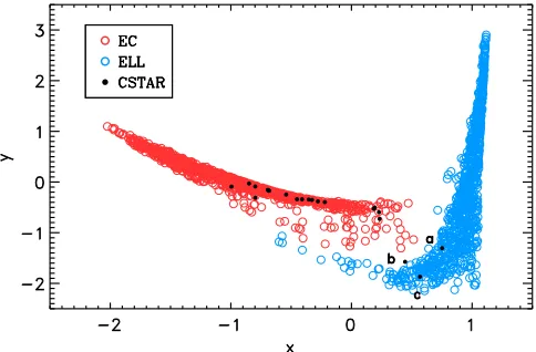
Figure 2.Two-dimensional LLE projection of the EC and ELL light curve space. Red and blue circles are sampled EC and ELL light curves, respectively. Black dots are light curves from CSTAR. Three CSTAR light curves fall into the ELL region:(a)CSTAR J100121.80-881330.8,(b)CSTAR J022530.81-871311.9, and (c) CSTAR J191753.08-885111.2. Note that the new coordinates(x, y)of each light curve do not depend on global translations, rotations, and scalings.

2

from USNO-B1.0 magnitudes to SDSS magnitudes. Because thefilters of CSTAR are similar to those of SDSS, the USNO-B1.0 catalog can be used to determine the photometric calibration directly. Time calibration was taken using the position of each star as a clock. The corrected Julian date(JD) at the mid-exposure point of every image was presented in each catalog. The accuracy can reach several seconds (Zhou et al.2010a).

Wang et al. (2012) correct the inhomogeneous effect of clouds on the CSTAR photometry, including the high cirrus and the fog near the ground surface. Meng et al.(2013)correct the ghost images, which are caused by the Schmidt–Cassegrain optical structure. As CSTAR wasfixed pointing to the Celestial South Pole, daily stellar movements in CCD will cause diurnal variation for each light curve due to the CCD unevenness. This has been removed by Wang et al. (2014a). After these corrections, the photometric precision can reach about 4 mmag ati=7.5 and 20 mmag ati=12(Wang et al.2014b). About 20,000 sources down to 16 mag were detected. The revised CSTAR catalog and data of 2008 are available athttp://explore. china-vo.org. The following work is based on the detrended light curves after these corrections.

3. ECLIPSING BINARY CATALOG

Eclipsing binaries are not easy to distinguish from other kinds of variables. Therefore, it is necessary to automatically search variables first and then manually select out eclipsing binaries from the variables. However, false positives caused by contaminating stars and the observation mode of CSTA may appear as a variable signature. They should be removed from the variable candidates before confirming eclipsing binaries. In this section, we describe the design of the eclipsing binary catalog.

3.1. Searching Periodic Signals

In thefirst step, periodic signals are extracted from each light curve. A bin size offive minutes has been adopted tofilter out extremely high-frequency noises because CSTAR has a very short cadence. Periodic signals are recognized using three methods: Lomb–Scargle (Lomb 1976; Scargle 1982), Phase

Dispersion Minimization (PDM; Stellingwerf 1978; Schwar-zenberg-Czerny1989), and Box Least Squares (BLS; Kovács et al. 2002). We set the range of period scan from 0.1 to 30 days for the PDM and BLS methods. Meanwhile, for the Lomb–Scargle method the lower limit is increased to 1.05 days. For each light curve, we calculate its Lomb–Scargle signal-to-noise ratio (S/N) R, PDM statistic Θ (see Stelling-werf 1978, Equation (3)), and Signal Detection Efficiency

(SDE; see Kovács et al.2002, Equation (6)). A false alarm probability (FAP) of 10−4 is assigned to the Lomb–Scargle method to obtain the power thresholdsLS. We set

s

=

R SLS LS,

where SLS is the power of the highest peak in the Lomb–

Scargle periodogram. A higher R value indicates more significant periodic signal. Θis between 0 and 1. A lowerΘ value indicates a more significant periodic signal. SDE can reflect the effective S/N of eclipses. This has been discussed in detail by Kovács et al.(2002). We choose the criteria

= Q = =

Rc 10, c 0.85, SDEc 6,

where the subscript “c” represents “criteria.” The Lomb– Scargle, PDM, and BLS methods contribute 225, 107, and 244 variable candidates, respectively. Ninety-three of them are detected using two methods and 27 are detected by all the three methods. Therefore, there are 429 variable candidates in total when any one of the condition is met.

3.2. Rejecting False Positives

False positives come from four sources. Thefirst source is diurnal variation. Though very weak after detrending, it still should be taken into consideration. Second, stars at the edges of the FOV have regular gaps because stars move in and out of the FOV repeatedly every day. This may cause additional periodic variations. Third, an exposure time of 20 or 30 s is too long for a bright variable star, which can pollute its neighborhood. A typical phenomenon is that they appear to have the same variations. Therefore, when two or more targets show nearly the same period, it is necessary to check if they are very close and if their light curves vary simultaneously. Additionally, a Table 1

Ellipsoidal Variables

CSTAR ID mag HJD Period

(JD-2454500) (days)

CSTAR J022530.81-871311.9 13.349(±0.031) 49.964260(±0.006070) 0.456869(±0.000035)

CSTAR J100121.80-881330.8 11.855(±0.014) 49.311958(±0.000269) 0.652239(±0.000002)

CSTAR J191753.08-885111.2 11.824(±0.014) 49.339306(±0000433) 0.372034(±0000002)

Note.Columns 1–4 represent CSTAR ID, magnitude, the reference time of the primary minimum, and period. J represents J2000.0.

Table 2

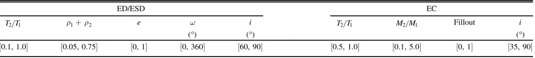
Ranges of Parameters

ED/ESD EC

T T2 1 r1+r2 e ω i T T2 1 M M2 1 Fillout i



( ) ( ) ( )

[0.1, 1.0] [0.05, 0.75] [0, 1] [0, 360] [60, 90] [0.5, 1.0] [0.1, 5.0] [0, 1] [35, 90]

Note.Columns 1–5 are parameter ranges of EDs and ESDs: temperature ratio, the sum of fractional radii, eccentricity, the argument of periastron, and inclination. Columns 6–9 are parameter ranges of ECs: temperature ratio, mass ratio,fillout factor, and inclination.

3

Table 3

Parameters of Eclipsing Detached Binaries

CSTAR ID mag HJD Period Crowding T T2 1 r1+r2 esinw ecosw sini

(JD-2454500) (days)

CSTAR J000116.84-874402.9 11.911(±0.015) 51.595627(±0.000812) 9.480642(±0.000146) 0.045 0.994 0.076 0.051 0.126 1.000 CSTAR J022528.30-875808.9 13.580(±0.033) 55.026981(±0.002729) 16.129131(±0.001444) 0.016 0.091 0.085 −0.382 0.295 0.999 CSTAR J031401.11-883253.1 14.491(±0.070) 50.940662(±0.001158) 1.208837(±0.000021) 0.087 0.565 0.260 0.027 −0.003 1.000 CSTAR J033130.30-880424.4 13.997(±0.050) 47.732536(±0.002857) 1.444413(±0.000062) 0.006 0.752 0.234 −0.117 0.000 0.993 CSTAR J061801.34-873953.9 13.371(±0.031) 55.336460(±0.017812) 6.048977(±0.001605) 0.009 0.940 0.114 −0.040 0.003 0.998 CSTAR J062842.76-880241.7 12.336(±0.017) 55.236904(±0.000568) 7.249134(±0.000062) 0.095 0.596 0.117 0.056 0.011 1.000 CSTAR J080846.28-880002.0 13.623(±0.034) 50.397514(±0.001443) 0.822784(±0.000016) 0.006 0.574 0.423 0.005 0.004 0.945 CSTAR J083940.85-873902.3 12.174(±0.016) 57.158970(±0.001962) 7.164405(±0.000241) 0.011 0.357 0.079 −0.256 0.063 0.999 CSTAR J090220.82-873741.0 12.355(±0.017) 44.738434(±0.004217) 1.627418(±0.000089) 0.022 0.542 0.555 0.199 −0.023 0.943 CSTAR J095836.02-882359.9 12.785(±0.020) 50.778557(±0.001152) 2.065943(±0.000035) 0.025 0.461 0.289 0.006 0.003 0.976 CSTAR J103232.73-882502.6 13.660(±0.023) 53.738533(±0.008547) 7.069140(±0.000943) 0.015 1.045 0.109 0.138 −0.001 0.998 CSTAR J104016.05-872929.8 11.102(±0.013) 49.466064(±0.000481) 0.868841(±0.000006) 0.032 0.821 0.425 −0.029 −0.001 0.948 CSTAR J130158.40-873956.3 8.984(±0.004) 55.650978(±0.000596) 5.800400(±0.000059) 0.003 0.825 0.208 0.057 −0.002 0.998 CSTAR J150537.60-873551.6 12.345(±0.016) 52.568558(±0.001329) 7.450763(±0.000322) 0.088 0.647 0.125 0.112 0.001 0.997 CSTAR J155705.55-873005.2 11.915(±0.014) 51.797089(±0.005051) 3.111666(±0.000207) 0.004 0.500 0.230 −0.332 −0.011 0.993 CSTAR J155917.54-880042.5 14.146(±0.056) 48.417747(±0.015527) 6.852954(±0.001552) 0.013 0.629 0.106 0.086 0.002 0.999 CSTAR J163136.82-874007.7 12.078(±0.015) 58.014969(±0.002532) 10.771624(±0.000552) 0.006 0.988 0.061 0.054 −0.001 1.000 CSTAR J183057.87-884317.5 9.839(±0.007) 53.714790(±0.002772) 9.922610(±0.000403) L L L L L L CSTAR J193827.80-885055.9 12.884(±0.021) 49.421947(±0.001194) 6.752321(±0.000111) 0.024 0.163 0.118 −0.139 −0.198 0.997 CSTAR J200218.84-880250.0 11.977(±0.015) 62.606724(±0.003508) 19.141005(±0.001177) 0.038 0.739 0.059 0.577 −0.357 1.000 CSTAR J202830.07-874616.5 11.805(±0.009) 51.365967(±0.000346) 2.192940(±0.000012) 0.000 0.417 0.340 0.196 −0.001 0.984 CSTAR J205410.67-890348.2 10.030(±0.008) 51.062473(±0.001411) 1.857557(±0.000038) 0.059 0.400 0.419 0.066 0.004 0.939 CSTAR J224601.56-880459.2 13.823(±0.040) 49.954193(±0.003384) 7.760361(±0.000409) 0.004 0.559 0.107 −0.013 0.005 0.999 CSTAR J235727.17-882454.5 12.396(±0.017) 50.875061(±0.002693) 6.199004(±0.000262) 0.008 0.291 0.131 0.007 −0.002 0.997

Note.Columns 1–10 represent CSTAR ID, magnitude, the reference time of primary minimum, period, crowding, temperature ratio, the sum of fractional radii, the radial component of eccentricity, the tangential component of eccentricity, and the sine of inclination. J represents J2000.0. The errors of the physical parameters follow the distributions as shown in Figure3.

4

The

Astrophysical

Journal

Supplement

Series,

217:28

(

16pp

)

,

2015

April

Y

ang

et

Table 4

Parameters of Eclipsing Semi-detached Binaries

CSTAR ID mag HJD Period Crowding T T2 1 r1+r2 esinw ecosw sini

(JD-2454500) (days)

CSTAR J074354.49-890737.3 12.538(±0.018) 49.325817(±0.000537) 0.797987(±0.000006) 0.007 0.481 0.669 0.003 0.006 0.948 CSTAR J084028.89-884700.4 13.807(±0.039) 52.206177(±0.029051) 13.027298(±0.004186) 0.001 0.828 0.723 0.001 −0.003 0.913 CSTAR J090359.29-883307.6 11.361(±0.013) 49.491791(±0.000177) 0.873754(±0.000002) 0.000 0.596 0.677 0.000 0.000 0.871 CSTAR J093334.26-865501.1 12.676(±0.022) 52.293953(±0.057799) 4.427421(±0.003756) 0.022 0.748 0.609 0.000 0.000 0.987 CSTAR J110803.52-870114.0 12.233(±0.017) 49.716991(±0.000752) 0.511559(±0.000005) 0.018 0.506 0.615 0.066 0.021 0.915 CSTAR J122135.82-880014.5 12.172(±0.016) 50.905312(±0.000439) 1.892200(±0.000011) 0.002 0.582 0.613 0.000 0.000 0.913 CSTAR J132349.26-881604.3 12.260(±0.016) 51.587410(±0.001441) 2.509739(±0.000051) 0.003 0.835 0.689 0.000 0.000 0.907 CSTAR J220502.55-895206.7 13.070(±0.023) 79.778481(±0.003821) 1.988110(±0.000091) 0.000 0.473 0.575 0.039 0.000 0.919

Note.Columns 1–10 represent CSTAR ID, magnitude, the reference time of primary minimum, period, crowding, temperature ratio, the sum of fractional radii, the radial component of eccentricity, the tangential component of eccentricity, and the sine of inclination. J represents J2000.0. The errors of the physical parameters follow the distributions as shown in Figure3.

5

The

Astrophysical

Journal

Supplement

Series,

217:28

(

16pp

)

,

2015

April

Y

ang

et

large plate scale of15 pix -1_{may also produce false eclipses}

induced by a nearby non-variable star. Other sources of contamination include solar brightness or moonlight at some epochs and the occasional aurora, all of which can brighten the sky background. Images with high background have been discarded in the data reduction process. Therefore, such contaminations have little effect.

All variable stars are checked in three ways. Their positions, periods, and variable trends are compared. False positives are confirmed if any one of the following conditions is met.

1. Distance less than 10 pixels to a saturated star. 2. Period equals one Sidereal Day or diurnal harmonics. 3. Variable trend resembles that of its neighborhood.

3.3. Classification of Eclipsing Binaries

All remaining light curves after culling false positives are manually inspected to exclude variables with similar shapes as eclipsing binaries, e.g.,γDoradus,δScuti, RR Lyrae, etc. To check if there exist eclipsing binaries in other types of variable stars, we subtract the strongest period of each variable star and analyze the residuals using the same method described above. A detached RS Canum Venaticorum variable is found as shown in Figure1.

The visual inspection of variables is carried out by two groups of authors (M. Yang et al. and S. Wang et al.) independently. Eclipsing binaries are selected out and classified into four types according to their morphologies (Paczyński et al.2006; Prša et al.2011):

1. Eclipsing Detached binary(ED)—neither componentfills its Roche Lobe;

2. Eclipsing Semi-detached binary(ESD)—only one com-ponentfills its Roche Lobe;

Table 5

Parameters of Eclipsing Contact Binaries

CSTAR ID mag HJD Period Crowding T T2 1 M M2 1 Fillout sini

(JD-2454500) (days)

CSTAR J005240.76-891732.4 13.997(±0.044) 51.531921(±0.000272) 0.292963(±0.000002) 0.006 0.941 0.287 0.898 0.959 CSTAR J031348.84-891511.7 13.047(±0.023) 49.405579(±0.000492) 0.344662(±0.000002) 0.011 0.922 0.646 0.016 0.598 CSTAR J042011.85-882503.5 12.647(±0.019) 55.389160(±0.000478) 0.395481(±0.000003) 0.001 1.008 1.012 0.842 0.714 CSTAR J051329.62-871942.6 11.939(±0.016) 75.154015(±0.000354) 0.384112(±0.000003) 0.003 0.987 0.483 0.570 0.893 CSTAR J051503.40-893226.6 14.431(±0.079) 49.452221(±0.001148) 0.358253(±0.000006) 0.002 0.954 0.272 0.953 0.910 CSTAR J061954.94-872047.5 12.399(±0.019) 49.499104(±0.001138) 0.491358(±0.000008) 0.000 0.759 0.892 0.364 0.631 CSTAR J064047.15-881521.3 11.721(±0.014) 49.455452(±0.000166) 0.438606(±0.000001) 0.003 0.988 0.849 0.856 0.936 CSTAR J071652.61-872856.4 13.472(±0.035) 50.483288(±0.000911) 0.383167(±0.000005) 0.007 0.936 0.508 0.943 0.909 CSTAR J073412.18-874037.3 13.218(±0.021) 50.181190(±0.000760) 0.331216(±0.000003) 0.000 0.858 0.531 0.984 0.828 CSTAR J084612.64-883342.9 11.997(±0.015) 49.312592(±0.000119) 0.267121(±0.000000) 0.003 0.921 1.077 0.872 0.960 CSTAR J123242.99-872622.8 11.100(±0.013) 49.395302(±0.000284) 0.338527(±0.000001) 0.003 0.975 1.256 0.973 0.983 CSTAR J124916.22-881117.6 13.834(±0.040) 55.331085(±0.000464) 0.352423(±0.000002) 0.002 0.998 0.889 0.788 0.883 CSTAR J135318.49-885414.6 12.783(±0.020) 49.365437(±0.000142) 0.266899(±0.000001) 0.004 0.978 1.087 0.922 0.959 CSTAR J142052.04-881433.4 12.599(±0.018) 49.326588(±0.000607) 0.400883(±0.000003) 0.000 0.970 0.979 0.254 0.498 CSTAR J142901.63-873816.2 13.542(±0.032) 55.409655(±0.000463) 0.348147(±0.000003) 0.004 0.699 1.293 0.532 0.830 CSTAR J181735.42-870602.2 10.819(±0.012) 49.649178(±0.002350) 0.352821(±0.000012) 0.001 0.703 1.398 1.082 0.796 CSTAR J195026.13-874450.7 12.832(±0.021) 49.474827(±0.000413) 0.416432(±0.000002) 0.002 1.022 0.792 1.017 0.879 CSTAR J223707.30-872849.9 11.624(±0.014) 50.040791(±0.001524) 0.848425(±0.000017) 0.005 0.910 1.058 1.014 0.959

Note.Columns 1–9 represent CSTAR ID, magnitude, the reference time of primary minimum, period, crowding, temperature ratio, mass ratio,fillout factor, and the sine of inclination. J represents J2000.0. The errors of the physical parameters follow the distributions as shown in Figure5.

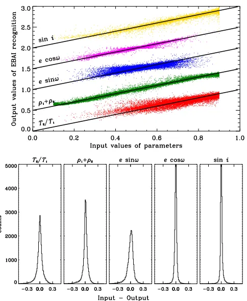
Figure 3. EBAI performance and parameter error distributions of simulated detached and semi-detached binaries. For accurate calculation, all the original parameters are linearly scaled to the[0.1, 0.9]interval by EBAI. The ranges of the original parameters are shown in Table2. Top panel: recognition results for 30,000 exemplars. TheXaxis represents the input values of parameters, and the

Yaxis represents the output values after recognition by EBAI. The parameters are offset by 0.5 in theYaxis for clarity. Bottom panels: error distributions of the parameters. The parameter errors are obtained by comparing the input values and the output values in the top panel.

6

3. Eclipsing Contact binary (EC)—both components fill their Roche lobes;

4. Ellipsoidal variable(ELL)—low-inclination binaries with close ellipsoidal components.

ED light curves are nearlyflat-topped with separate eclipses. ESD light curves are continuously variable with a large difference in depth between the primary and the secondary eclipses. Therefore, detached and semi-detached systems are easy to be recognized due to their distinct eclipses. However, for a contact system with indistinct ingress and egress points of the eclipses, visual inspection is not reliable. Challenges mainly come fromδScuti variables and ELLs because bothδScuti and ELL light curves exhibit sinusoidal variations. If a contact system appears with approximately equal primary and secondary eclipses, it is difficult to distinguish the EC light

curve from the δ Scuti and ELL light curves. We adopt the methods of frequency spectrum analysis and the Locally Linear Embedding(LLE; Roweis & Saul2000)technique to solve the problem.

The frequency spectra of ECs and δScutis are different. δ Scuti light curves exhibit variations due to both radial and non-radial pulsations of the star’s surface. Therefore, the frequency spectrum of aδScuti usually contains more peaks caused by multi-mode pulsations. On the other hand, the frequency spectrum of an EC light curve contains only one strong signal and harmonics of the signal. For CSTAR data with a short cadence of ∼30 s, the harmonics are usually very weak. We calculate the frequency spectra of all sinusoidal variables using the Lomb–Scargle method from 0.025 day to 0.95 day for further reference.

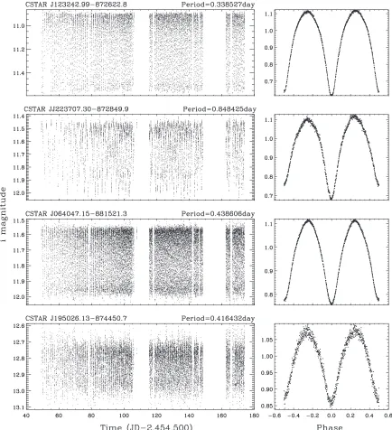
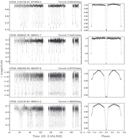
Figure 4.Example light curves of detached and semi-detach systems. The left-hand panels show the star brightness in magnitudes during the whole observation season. The right-hand panels show the phased and binned light curves in relativeflux. CSTAR IDs and periods are given on top of every light curve.

7

ELL light curves exhibit sinusoidal variations due to the changing emitting area toward the observer. We adopt the LLE method proposed by Matijevičet al.(2012)to distinguish ECs and ELLs. LLE is a nonlinear dimensionality reduction technique. This method has been applied to KEPLER data to classify eclipsing binary light curves and has turned out to be successful. LLE can remember the local geometry of a higher-dimensional data set and reconstruct a lower-higher-dimensional projection with the same local geometry. Therefore, light curves with similar features will stay adjacent to each other in the lower dimensional projection. We generate 1000 EC light curves and 1000 ELL light curves using the PHOEBE package, respectively. The amplitudes of these light curves are scaled to the [0, 1] interval. The light curves are sampled at 100 equidistant phases; in other words, each light curve can be treated as a point in aD=100 dimensional space. To preserve the local geometry, every light curve is characterized by a linear combination of its k = 20 neighbors. We reduce the

D=100 dimensional space to ad=2 dimensional space. The final two-dimensional LLE projection is shown in Figure 2. Each point represents a light curve sampled at 100 equidistant phases. Sampled EC light curves(red circles)are clustered in the red region, and sampled ELL light curves (blue circles)in blue region. Three light curves fall into the ELL region. They are listed in Table1. The periods and ephemerides of the ELLs are derived in Section4.

Combining visual inspection, frequency spectrum analysis, and the LLE technique, eclipsing binaries are selected out and voted on by all members. Finally, 53 systems are classified into 24 EDs (45%), 8 ESDs (15%), 18 ECs (34%), and 3 ELLs

(6%). Compared with other projects, the fractions of different types of eclipsing binaries from the University of New South

Wales (UNSW) Extrasolar Planet Search are 43.1% for EDs and ESDs, and 56.9% for ECs (Christiansen et al. 2008);

Keplerfractions are58.2%for EDs, 7% for ESDs,21.7%for ECs, 6.3% for ELLs, and6.8% for uncertain types(Slawson et al. 2011). The longer observation time and unprecedented precision ofKepler make it sensitive to long-period EDs. Our result lies between the two projects.

4. ECLIPSING BINARY PARAMETERS

In this section, we give the binary parameters as shown in Tables2–5. Two methods are applied to determine the accurate periods and ephemerides. The first one is the classical O-C method. Epochs of minimum light are given by the K-W method(Kwee & van Woerden1956). Then, a linearfit of the epochs is performed to derive the period and ephemeris as described by Zhang et al.(2014). For the second method, prior to the linear fit, we adopt a polynominal fit to determine the epochs of the light minima instead of the K-W method. Details are described in Section5.1. These two methods are performed separately and the results with higher precisions are adopted.

With the previously obtained periods and ephemerides, the physical parameters of these eclipsing binaries are computed using the EBAI method. EBAI introduces artificial neural networks to learn the characteristics by training on large data sets. Then, the knowledge is applied to recognize the physical parameters of new eclipsing binaries. Prša et al.(2008)have described the principles of the method. Test results of applying it to EDs from the CALEB and OGLE database point to significant viability. Prša et al. (2011) and Slawson et al.

(2011)have discussed how to choose principal parameters for ED, ESD, and EC(see Prša et al. 2011, Table 2). We use the parameters they recommended. First, we ran the PHOEBE package to generate modeled eclipsing binary light curves for the training process. PHOEBE is a modeling package for eclipsing binaries based on the Wilson–Devinney program. It retains all Wilson–Devinney codes as the lowermost layer, the extension of physical models and technical solutions as the intermediate layer, and the user interface as the topmost layer. Parameters for different types of eclipsing binaries are calculated with different methods.

4.1. Parameters of Detached and Semi-detached Binaries

For EDs and ESDs, we choosefive principal parameters: the temperature ratioT2 T1, which determines the eclipse depth

ratio; the sum of fractional radii r₁+r₂, which determines eclipse width; the eccentricityeand the argument of periastron

ωin orthogonal formse· sinwande· cosw, which determine the separation between primary and secondary eclipse; and the sine of inclinationsini, which determines the eclipse shape. We generate 30,000 simulated light curves by randomly sampling thefive parameters as a training set for EBAI. After 200,000 training iterations, a correlation matrix which can recognize parameters from eclipsing binary light curves is generated. We test the correlation matrix with 30,000 unknown light curves. The recognition results and the parameter error distributions are shown in Figure 3. All the parameters have been linearly scaled to the [0.1, 0.9] interval by EBAI. The ranges of the parameters are shown in Table2.

We fold the observed light curves to one period, normalize theflux and time, andfit the profiles with a bin size which is the same with the modeled light curves. Parameters are obtained Figure 5.Similar to Figure3but for ECs. The parameters are linearly scaled to

the[0.1, 0.9]interval by EBAI. Their actual ranges are given in Table2.

8

rapidly by applying the trained EBAI matrix to the folded light curves, as shown in Tables3and4. The light curve of CSTAR J183057.87-884317.5 only shows primary eclipses. However, it has been found as an ED system with a high radial velocity amplitude of 12 km s−1by Wang et al.(2014b). We list it in the ED catalog but do not calculate its parameters. Figure 4 illustrates some ED and ESD light curves. The left-hand panels show the star brightness in magnitudes during the whole observation season. The right-hand panels show the phased and binned light curves in relativeflux. Periods and CSTAR IDs are given at the top of every left-hand panel.

4.2. Parameters of Contact Binaries

For ECs, there is no handle on eccentricity and argument of periastron. Instead, the lobe-filling configuration of a contact

system links the Roche model with the radii of the components. As a result, the photometric mass ratioq can be estimated. In order to describe the contact degree, thefillout factorFis given by Prša et al.(2011):

=

-F Ω Ω

Ω Ω , (1)

L

L L

2

1 2

whereΩ(see Wilson & Devinney1971, Equation(1))is the surface potential of the common envelope,ΩL1is the potential at the inner Lagrangian surface, andΩL2is the potential at the outer Lagrangian surface. A star in a contact system will transfer mass to its companion through the the inner Lagrangian point L1, or lose mass through the the outer

Lagrangian pointL2.

Figure 6.Example light curves of contact systems. CSTAR IDs and periods are given on top of every light curve.

9

From the above consideration, four principal parameters are chosen for EC:T2 T1,q,F, andsini. The network is trained on

20,000 simulated light curves for 1,000,000 iterations. We test the correlation matrix with 10,000 unknown EC light curves. The recognition results and the parameter error distributions are shown in Figure5. We apply the correlation matrix to EC light curves of CSTAR. The parameters are given in Table 5. Figure6shows some EC light curves.

5. ECLIPSE TIMING VARIATIONS

Companions are common around binary stars. It is suggested that close binaries are formed as a result of tidal friction and Kozai cycles in a multiple-star system (Bonnell 2001; Fabrycky & Tremaine2007). Spectroscopic observations also support such a scenario (Tokovinin 1997; Tokovinin et al. 2006). The perturbation of the tertiary companion may change the eclipse mid-times. By calculating ETVs, we may find the tertiary companion. Other origins contributing to ETVs include star spots, mass transfer, spin–orbit transfer of angular momentum, and orbit precession. The spin–orbit transfer of angular momentum is ignored in this paper because it changes the eclipse mid-times on the order of 10−5of the orbital period

(Applegate1992). The eccentricities of our short-period ECs and ESDs are close to zero due to tidal friction. Therefore, their orbit precession can also be ignored. ETVs caused by star spots are discussed in Section5.2. We do not calculate ETVs for EDs because of limited eclipses during the observation span.

5.1. Computing Method of ETVs

To estimate the primary eclipse mid-times, a simple linear increment is applied with known eclipse epoch and period. Then, the whole light curve is divided into many small segments. Each segment centers around a primary eclipse mid-Figure 7. Primary (blue), secondary (red), and synthetic(black)ETVs of

CSTAR J220502.55-895206.7. The synthetic ETV is half of the sum of the primary and secondary ETVs. The parameters of the third body are derived by fitting Equation(5)with Synthetic ETV. ETV data are marked usingfilled circles with error bars, and thefit result of the synthetic ETV is marked using a thick line.

Figure 8.Anti-correlated primary(blue)and secondary(red)ETVs of CSTAR J122135.82-880014.5(top)and J132349.26-881604.3(bottom). Primary and secondary ETVs arefitted using Equation (3), respectively. ETV data are marked usingfilled circles with error bars, andfit results are marked using thick lines.

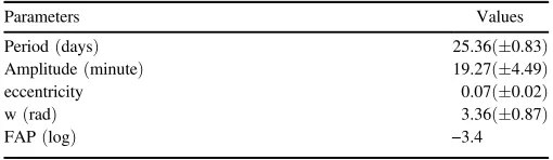
Table 6

Parameters of the Potential Companion around CSTAR J220502.55-895206.7

Parameters Values

Period(days) 25.36(±0.83)

Amplitude(minute) 19.27(±4.49)

eccentricity 0.07(±0.02)

w(rad) 3.36(±0.87)

FAP(log) −3.4

10

time. We exclude segments with fewer points because such segments can reduce the fit precision. To obtain the eclipse template, we fold all of the remaining segments. The template isfit using the following function(see Rappaport et al.2013, Equation(2)):

a b

= - + - +

f (t t0)2 (t t0)4 f0, (2)

where f is the eclipse flux, f0 is the minimum flux, t is the

eclipse time, andt0is the eclipse mid-time. Observed mid-times

are obtained by comparing each segment with the theoretical template. All the other parameters except the eclipse mid-time are fixed to be the same as the template when comparing. A linearfit is applied to all of thefitted mid-times. The differences between the fitted mid-times and their linear trend are ETVs.

The same processes are applied to secondary eclipses to derive secondary ETVs.

5.2. Analysis of ETVs

The relationship between the primary and the secondary ETVs for a binary system may be correlated or anti-correlated. The correlation can be explained with a tertiary companion(Conroy et al.2014)and the anti-correlation may be attribute to sunspots

(Tran et al.2013). However, when observed ETVs are less than one cycle, it is necessary to consider the probability of mass transfer. Conroy et al. (2014) adopt a Bayesian Information Criterion to distinguish between the two cases.

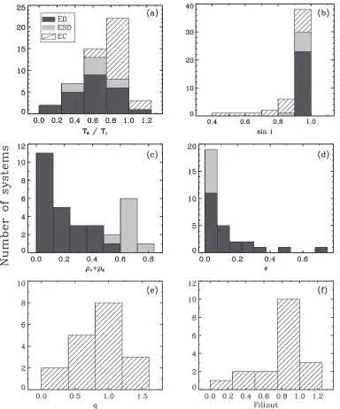
To check the relationship between the primary and the secondary ETVs, we choose a similar method as for searching planets (Steffen et al. 2012). ETVs are fitted using the Figure 9.Statistics of the number of eclipsing binaries with different physical parameters:(a)temperature ratio,(b)the sine of orbital inclination,(c)the sum of fractional radii,(d)eccentricity,(e)mass ratio, and(f)fillout factor.

11

following function(see Ming et al.2013, Equation(2)):

= æ

è ççç öø÷÷÷ +

æ è

ççç öø÷÷÷ + +

f A πt

P B

πt

P Ct D

sin 2 cos 2 , (3)

where A,B,C, andD are model parameters andP is the test period.P is increased from 20 to 100 days with a step of 0.1 day. The degree of correlation is estimated by

s s s s

X( )P = A Ap s + B B , (4)

A A

p s

B B

p s p s

where the subscript“p”represents“primary”and“s”represents

“secondary”;sA,sB,sC, andsDare the uncertainties ofA,B,C,

and D. The maximum ∣ ∣X is adopted, which represents the degree of correlation. Positive Ξ represents correlation and negative Ξ represents anti-correlation. To confirm correlated ETVs, we calculate the FAPs by a bootstrap randomization process: the ETVs are randomly scrambled 104times to obtain the corresponding X¢max. The proportion of X¢max larger than

Xmax represents the FAP. Induced periods are calculated to

exclude the effect of sampling cadence. Finally, two systems pass the FAP criteria of 10−3. CSTAR J084612.64-883342.9 has a FAP lower then 10−4and CSTAR J220502.55-895206.7 has a FAP of about10-3.4. Qian et al.(2014)also claimed that a third body may exist around CSTAR J084612.64-883342.9. Figure 7 shows correlated ETVs of CSTAR J220502.55-895206.7 and Figure 8 shows anti-correlated ETVs. For a correlated system, we sum its primary and secondary ETVs and divide the sum by two as the synthetic ETV of the binary system. If there is only a primary eclipse or only a secondary eclipse in one orbital period, then the ETV of the available eclipse is approximated as the synthetic ETV directly. To derive the parameters of the third companion, the synthetic ETV isfitted using a triple-star model (Rappaport et al. 2013; Conroy et al.2014):

w

w

= é ë ê

-+ - ù_û

(

)

(

)

A e u t

u t e

ETV 1 sin ( ) cos

cos ( ) sin , (5)

3 2 1 2

3 3

3 3 3

Figure 10.Example light curves of eccentric detached binaries. The light curves are folded and binned to 5000 points. CSTAR IDs are given at the top of each panel.

Figure 11.Eccentricities and orbital periods of the detached and semi-detached binaries. The black line is the upper envelope derived by Mazeh (2008)to constrain the binary region. All 2751 binaries from the SB9 catalog are used to obtain the expression of the upper envelope. EDs and ESDs in this paper are marked with black dots.

12

where

= +

u t3( ) M t3( ) e3sinu t3( ), (6)

=

-M t t t π

P

( ) ( )2 , (7)

3 0

3

= é

ë ê ê

ù

û ú ú

A G

c π m

m i P

(2 )

sin , (8)

LTTE

1 3

2 3 3

1232 3

3 32 3

where subscript “3” represents the third companion,A is the amplitude, e3 is eccentricity, P3 is orbital period, u t3( ) is

eccentric anomaly,M t3( )is mean anomaly,i3is inclination,w3

is argument of periastron, and m123 is the mass of the whole

system. The parameters we choose to give areA,e3,P3, andw3.

We fix the period corresponding to the maximum Ξ. Other parameters are changeable. For a more reliablefit, we choose the Markov Chain Monte Carlo method instead of the Figure 12.Light curves with O’Connell effect∣Dm∣ ⩾0.01.D =m mII-mIin the lower left of each panel represents the difference between the maxima, wheremI

is the peak magnitude after primary minimum andmIIis the peak magnitude after secondary minimum. The light curves are folded and binned to 5000 points. CSTAR

IDs are given at the top of each panel.

13

Levenberg–Marquardt algorithm. The results are shown in Table6.

6. RESULTS

We identify and classify 53 eclipsing binaries, containing 24 EDs, 8 ESDs, 18 ECs, and 3 ELLs. The distributions of their physical parameters are shown in Figure9. Some EDs may be in the dynamically hot stage because of high eccentricities. We plot four EDs with eccentricities higher than 0.1 (CSTAR J000116.84-874402.9, J200218.84-880250.0, J083940.85-873902.3, and J193827.80-885055.9) in Figure 10 and give the period-eccentricity diagram in Figure11. Many folded light curves present asymmetry in brightness as shown in Figure12. ETV analyzes the present systems with correlation and anti-correlation between the primary and the secondary eclipses, respectively. The systems mentioned above are discussed as follows.

6.1. Binary Parameters and Typical Characteristics

Eclipsing binary parameters are given in Tables 3–5. The distributions of the physical parameters (see Table 2) are shown in Figure 9. Because samples in this paper are limited, we use a large bin size to test some typical characteristics.

For detached and semi-detached systems, the eclipse depth ratio reflects the temperature ratio. In equal depth eclipses, its value is one. The temperature ratios of the EDs and ESDs in this paper center around a value lower than one. Prša et al.

(2011)explain that it is because the orbital eccentricity and star radii can affect the eclipse depth, thus increasing the scatter when the temperature ratio approaches one. The inclinations are close to 90°for detached and semi-detached systems. This is because eclipses can only be seen in the edge-on geometrical configuration when the two components are not very close. The sum of the fractional radii distribute around 0.1 for EDs and 0.6 for ESDs.

What is interesting for EDs and ESDs is their eccentricity distribution. Most of the eccentricities are close to zero. However, the highest eccentricity can reach 0.679 (CSTAR J200218.84-880250.0). Hut(1981)analyzes the tidal evolution of binaries and concludes that the timescale of circularization can be a relatively slow process. Mazeh (2008) plots the eccentricities as a function of the orbital periods using all 2751 binaries from the official IAU catalog of spectroscopic binaries

(SB9). He derives an“upper envelope”to constrain the binary eccentricity(see Mazeh2008, Equation(4.4)):

= -

₍

₎

f P( ) E Aexp (pB)C , (9)

whereE=0.98,A=3.25, B=6.3, andC=0.23. The EDs and ESDs in this paper are all below the upper envelope as shown in Figure 11. Two detached systems (CSTAR J200218.84-880250.0 and J022528.30-875808.9)at the upper right of Figure11have longer periods and larger eccentricities. Such systems have experienced less of the circularization process. Therefore, they are important to investigate how the circularization process can affect the binary components by comparing high-eccentricity binaries with circular binaries

(Shivvers et al.2014).

For contact systems, the two lobe-filling components can transfer mass to each other through the inner Lagrangian point. They can easily reach a thermal contact because of the common envelope. Therefore their temperature ratios center around one as shown in Figure9(a). The relatively larger size of the Roche lobe also relax the limitation of edge-on geometrical require-ment. ECs with lower inclinations can be detected as shown in Figure9(b). The photometric mass ratios of ECs peak at 1. The fillout factors for the ECs are not roughly uniform because overcontact systems and close-to-contact systems contribute to the peak at 1.

6.2. Light Curves with O’Connell Effect

Many CSTAR phased light curves of ECs and ESDs appear different maxima in brightness as shown in Figure 12. These light curves have been phased and binned to 5000 equally spaced points. Such a phenomenon is called the O’Connell effect (O’Connell 1951; Davidge & Milone 1984). The O’Connell Effect can be quantitatively expressed by measuring the difference between the two out-of-eclipse maxima

D =m mII-mI, (10)

where mI and mII are the peak magnitude after primary

minimum and secondary minimum, respectively. To derivemI

andmII, we fold each light curve with its orbital period andfit

the parts centered around each maximum using Equation(2). Table7presents the contact and semi-detached systems with D

∣ m∣greater than 0.01. Nearly half of the contact systems are listed in this table. Therefore, the O’Connell Effect is common among eclipsing binary systems. The reasons for O’Connell effect are still debatable. Mullan (1975) proposed that large toroidal magneticfields may be generated because of enforced rapid rotation in deep convection zones of contact binaries. The toroidal magnetic fields can cause active low-temperature zones, namely, spots. The spots can be used to explain the reason for the O’Connell effect. However, not all the ESDs have deep convection zones like the ECs. Instead, they may Table 7

Contact and Semi-detached Systems with the O’Connell Effect

CSTAR ID _Dm Type CSTAR ID _Dm Type

(mag) (mag)

CSTAR J031348.84-891511.7 0.015 EC CSTAR J061954.94-872047.5 0.036 EC

CSTAR J071652.61-872856.4 −0.016 EC CSTAR J073412.18-874037.3 0.015 EC

CSTAR J084612.64-883342.9 −0.022 EC CSTAR J124916.22-881117.6 0.015 EC

CSTAR J135318.49-885414.6 0.023 EC CSTAR J142901.63-873816.2 0.024 EC

CSTAR J181735.42-870602.2 −0.019 EC CSTAR J223707.30-872849.9 0.017 EC

CSTAR J110803.52-870114.0 0.030 ESD CSTAR J132349.26-881604.3 0.037 ESD

CSTAR J220502.55-895206.7 0.022 ESD L L L

Note.D =m mII-mI, wheremIis the peak magnitude after primary minimum andmIIis the peak magnitude after secondary minimum.

14

have hot spots because of mass transfer. In addition, the O’Connell effect can also be found in some EDs. Davidge & Milone (1984) have discovered that the O’Connell effect of detached systems is significantly correlated with the color index. Therefore, the O’Connell effect may be caused by more than one mechanism. More eclipsing binaries with a different color index are needed to study it.

6.3. ETVs for Binaries

ETVs are useful for studying the apsidal motion, mass transfer and loss, solar-like activities in late-type stars, light-time effect of a third companion, etc. They are helpful in understanding the formation and evolution of binary systems. The light curves of short-period binaries from Antarctica are available for tens of days thanks to the polar nights. Therefore, their ETVs are more continuous.

We only calculate ETVs for semi-detached and contact binaries. The spin–orbit transfer of angular momentum

(Applegate 1992)does not create observable signals because their orbital periods are very short and the best precision of our ETVs is one minute, as shown in Figure 7. Apsidal motion is ignored because the eccentricities of semi-detached and contact binaries are close to zero.

Systems with potential large spots are shown in Figure8. For each system, we can see obvious anti-correlation between the primary and the secondary eclipses. We find two eclipsing binary systems with a potential third body: CSTAR J084612.64-883342.9 and CSTAR J220502.55-895206.7. Recently, Qian et al. (2014) also claimed that CSTAR J084612.64-883342.9 is a triple system and derived the parameters of the third body with more observations(see Qian et al.2014, Table 5). In this paper, we analyze the other system CSTAR J220502.55-895206.7. The ETVs of CSTAR J220502.55-895206.7 are given in Figure 7. The parameters of the close-in third body are given in Table 6. The orbital period of the third body is 25.36 days, indicating a close distance from the binary. Because the mass of the third companion and the orbital inclination are coupled in the amplitude, we cannot discern the nature of the third companion.

7. CONCLUSIONS

CSTAR, with an aperture of 14.5 cm (effective aperture 10 cm), was fixed to point in the direction near the Celestial South Pole at Dome A. After analyzing i-band data of CSTAR observed in 2008, a master catalog containing 22,000 sources was obtained. There are about 20,000 sources between 8.5 and 15 mag. The polar night condition of Dome A and the large aperture of CSTAR make it more suitable to search and analyze eclipsing binaries.

In this work, we analyze each light curve using the Lomb– Scargle, PDM, and BLS methods to search variables. To pick out binaries from the variables, the period, the CCD position, and the morphology of the light curves are compared and checked. Finally, we discover53eclipsing binaries in the FOV of CSTAR. Therefore, the binary occurrence rate is 0.26% concerning the ∼20,000 sources in the master catalog. It is lower compared with 0.8%ofHipparcosand1.2%ofKepler, but close to the OGLE binary occurrence rate of 0.2%for all stars. There are more EDs and ESDs than ECs, as indicated by

Kepler.

The parameters of the eclipsing binaries are calculated using the PHOEBE package and EBAI pipeline. For different types of eclipsing binaries, we choose different parameters. The general statistical characteristics of the parameters are similar with KEPLER. Since the number of eclipsing binaries in this paper is limited, it is not possible to investigate detailed statistical characteristics. However, individual systems on the edge of the parameter distributions are still of concern. Some detached binaries are found to be very eccentric. We check their eccentricities in the period-eccentricity diagram offered by Mazeh (2008), and the eccentricities are all within the restricted area. An eccentric binary orbit indicates a dynamical hot stage. Therefore, such systems are valuable to study the evolution of binaries and the impact of the circularization process on binary components.

Antarctic polar nights also offer good opportunities to investigate light curves continuously and in detail. For short-period variables, observations can be taken during the whole orbital period without interruption. Therefore, it is very efficient to analyze the variations of some physical quantities, such as ETV. We calculate the ETVs for all semi-detached and contact systems. The precision of CSTAR ETVs can achieve 1 minute at 9 mag, which can reveal the existence of a massive third companion. The ETV analyses present (1) two systems with correlated primary and secondary ETVs, implying potential companions; and (2)another two systems with anti-correlated primary and secondary ETVs, implying star spots. The orbital parameters of the third boy in system CSTAR J220502.55-895206.7 are derived using a triple-star dynamical model.

We are grateful to Andrej Prša for helpful discussions and for sharing his PHOEBE script with us. We thank Xiaobin Zhang and Changqing Luo for their helpful comments. We sincerely appreciate the crew involved in the CSTAR project and the Chinese Antarctic Science team who delivered and set up CSTAR at Dome A for thefirst time. We are also grateful to the High Performance Computing Center(HPCC)of Nanjing University for doing the numerical calculations in this paper on its IBM Blade cluster system. This research has been supported by the Key Development Program of Basic Research of China

(No. 2013CB834900), the National Natural Science Founda-tions of China (Nos. 10925313, 11003010, and 11333002), Strategic Priority Research Program “The Emergence of Cosmological Structures”of the Chinese Academy of Sciences

(grant No. XDB09000000), the Natural Science Foundation for the Youth of Jiangsu Province (No. BK20130547), Jiangsu Province Innovation for PhD candidate(No. KYZZ_0030 and KYLX_0031), 985 Project of Ministration of Education and Superiority Discipline Construction Project of Jiangsu Province.

REFERENCES

Alcock, C., Allsman, R. A., Alves, D., et al. 1997,AJ,114, 326 Andersen, J. 1991, A&ARv,3, 91

Applegate, J. H. 1992,ApJ,385, 621

Bonnell, I. A. 2001, in IAU Symp. 200, The Formation of Binary Stars, ed. H. Zinnecker, & R. D. Mathieu(San Francisco, CA: ASP),23

Borucki, W., Koch, D., Boss, A., et al. 2004, in Stellar Structure and Habitable Planet Finding, ed. F. Favata, S. Aigrain, & A. Wilson(ESA SP-538; Noordwijk: ESA),177

Christiansen, J. L., Derekas, A., Kiss, L. L., et al. 2008,MNRAS,385, 1749 Conroy, K. E., Prša, A., Stassun, K. G., et al. 2014,AJ,147, 45

Davidge, T. J., & Milone, E. F. 1984,ApJS,55, 571

15

Doyle, L. R., Carter, J. A., Fabrycky, D. C., et al. 2011,Sci,333, 1602 Fabrycky, D., & Tremaine, S. 2007,ApJ,669, 1298

Guinan, E. F., Ribas, I., Fitzpatrick, E. L., et al. 2000,ApJ,544, 409 Hut, P. 1981, A&A,99, 126

Kallrath, J., & Milone, E. F. 1999, Eclipsing Binary Stars: Modeling and Analysis(New York: Springer)

Kovács, G., Zucker, S., & Mazeh, T. 2002,A&A,391, 369 Kwee, K. K., & van Woerden, H. 1956, BAN,12, 327

Lawrence, J. S., Allen, G. R., Ashley, M. C. B., et al. 2008,Proc. SPIE,7012, 701227

Lawrence, J. S., Ashley, M. C. B., Hengst, S., et al. 2009, RScI,80, 064501 Lomb, N. R. 1976,Ap&SS,39, 447

Matijevič, G., Prša, A., Orosz, J. A., et al. 2012,AJ,143, 123 Mazeh, T. 2008,EAS Publications Series,29, 1

Meng, Z., Zhou, X., Zhang, H., et al. 2013,PASP,125, 1015 Milone, E. E. 1968,AJ,73, 708

Monet, D. G., Levine, S. E., Canzian, B., et al. 2003,AJ,125, 984 Mullan, D. J. 1975,ApJ,198, 563

O’Connell, D. J. K. 1951, PRCO,2, 85

Orosz, J. A., Welsh, W. F., Carter, J. A., et al. 2012a,ApJ,758, 87 Orosz, J. A., Welsh, W. F., Carter, J. A., et al. 2012b,Sci,337, 1511 Paczyński, B., Szczygieł, D. M., Pilecki, B., & Pojmański, G. 2006, MNRAS,

368, 1311

Pojmanski, G. 2002, AcA,52, 397 Prša, A., & Zwitter, T. 2005,ApJ,628, 426

Prša, A., Batalha, N., Slawson, R. W., et al. 2011,AJ,141, 83 Prša, A., Guinan, E. F., Devinney, E. J., et al. 2008,ApJ,687, 542 Pols, O. R., Tout, C. A., Schroder, K.-P., Eggleton, P. P., & Manners, J. 1997,

MNRAS,289, 869

Pustylnik, I. B. 2005,Ap&SS,296, 69

Qian, S.-B., Wang, J.-J., Zhu, L.-Y., et al. 2014,ApJS,212, 4 Rappaport, S., Deck, K., Levine, A., et al. 2013,ApJ,768, 33 Roweis, S. T., & Saul, L. K. 2000, Sci,290, 2323

Saunders, W., Lawrence, J. S., Storey, J. W. V., et al. 2009,PASP,121, 976 Scargle, J. D. 1982,ApJ,263, 835

Schwarzenberg-Czerny, A. 1989,MNRAS,241, 153

Shivvers, I., Bloom, J. S., & Richards, J. W. 2014,MNRAS,441, 343 Slawson, R. W., Prša, A., Welsh, W. F., et al. 2011,AJ,142, 160

Steffen, J. H., Fabrycky, D. C., Ford, E. B., et al. 2012,MNRAS,421, 2342 Stellingwerf, R. F. 1978,ApJ,224, 953

Tokovinin, A. A. 1997, AstL,23, 727

Tokovinin, A., Thomas, S., Sterzik, M., & Udry, S. 2006,A&A,450, 681 Torres, G., & Ribas, I. 2002,ApJ,567, 1140

Tran, K., Levine, A., Rappaport, S., et al. 2013,ApJ,774, 81 Udalski, A., Kubiak, M., & Szymanski, M. 1997, AcA,47, 319 Wang, L., Macri, L. M., Krisciunas, K., et al. 2011,AJ,142, 155 Wang, L., Macri, L. M., Wang, L., et al. 2013,AJ,146, 139 Wang, S.-H., Zhou, X., Zhang, H., et al. 2014a,RAA,14, 345 Wang, S., Zhang, H., Zhou, J.-L., et al. 2014b,ApJS,211, 26 Wang, S., Zhou, X., Zhang, H., et al. 2012,PASP,124, 1167 Welsh, W. F., Orosz, J. A., Carter, J. A., et al. 2012,Natur,481, 475 White, R. J., & Ghez, A. M. 2001,ApJ,556, 265

Wilson, R. E., & Devinney, E. J. 1971,ApJ,166, 605

Yang, H., Allen, G., Ashley, M. C. B., et al. 2009,PASP,121, 174 Yang, M., Liu, H.-G., Zhang, H., Yang, J.-Y., & Zhou, J.-L. 2013, ApJ,

778, 110

Zhang, X. B., Deng, L. C., Wang, K., et al. 2014,AJ,148, 40 Zhou, X., Fan, Z., Jiang, Z., et al. 2010a,PASP,122, 347 Zhou, X., Wu, Z.-Y., Jiang, Z.-J., et al. 2010b,RAA,10, 279 Zou, H., Zhou, X., Jiang, Z., et al. 2010,AJ,140, 602

16