A local field correlated and Monte Carlo based shallow neural network model for nonlinear time series prediction

Time series forecasting has remained a challenging prob-lem in environmental research. Since the late 1980, not only shallow neural networks but also multi-layer perceptions (MLP)have been widelydeployed totimeseries forecasting. Later on, feed-forward neural networks and support vector machinesarewelldeveloped.Inthepastyears,deeplearning, which was derived from multi-layer perceptions, has been consideredasamostbrain-likeartificialneuralnetworkandis appliedtomanyapplicationfieldsinmachinelearninganddata analysis.Simultaneously alotof algorithms aimingtodesign an efficientartificialneural networkhave alsobeen proposed andbeen adopted tocorresponding data sets, such as “Back-Propagation”, “Extreme Learning Machine” and “Boltzmann”[1]. Neural network model is suitable for analyzing internal relations in dealing with a variety of data, not only in pattern recognition, but also in time series forecasting. It has been considered as a powerful tool to solve the problems including classification, forecasting in most of the areas, such as com-puter vision, text mining, ubiquitous computing[2] and also web service[3, 4]. A proper design of ANN models could also serve as a robust and efficient tool in water resources modeling and forecasting [5].

Most of the ancient civilizations have made use of wells, spring water and groundwater since theBronze Age [6]. Groundwater is being considered as the most valuable natural resources in the future, and it becomes more importantformanydifferentclimaticregionsallovertheworld [7]. Nowthat groundwatersupply isbeing indanger, howto make asustainable management of groundwaterresources is by farthe utmostimportant issuefor us.Groundwater usein irrigationisavitalprobleminmanyaridandsemi-aridregions especially when we take adeep lookin the HeiheRegion in Gansu Province of China. In this paper, we mainly focus on theHeiheRegion andallthe datarangesfrom1986to2008.

As model validation is a main tool in optimization, for groundwater management there are several models being used to help optimizing groundwater usage [8]. Box-Jenkins Model [9], ANN, autoregressive integrated moving average (ARIMA) [10] and Physical Based Model [11] are used for groundwater research including time series forecasting.

In this paper, we proposed a new algorithm for conventional artificial neural network, which was different from Back Propagation, SVM and others. With its simple architecture and powerful performance, we have shown its experimental result in the Heihe River dataset. The rest of the paper was organized as follows. In next section, we will review the Box-Jenkins Model, ARIMA model, Physical Based Model and

on Scalable Information Systems

Research Article

A Local Field Correlated and Monte Carlo Based

Shallow Neural Network Model for Nonlinear

Time Series Prediction

Qingguo Zhou

, Huaming Chen

_{, Hong Zhao}

_{, Gaofeng Zhang}

, Jianming Yong

_{and Jun Shen}

*

Corresponding author. Email: [email protected]

Received on 01December 2015, accepted on 05 June 2016, published on 09 August 2016

Copyright © 2016 Vimalachandran et al., licensed to EAI. This is an open access article distributed under the terms of the Creative Commons Attribution licence (http://creativecommons.org/licenses/by/3.0/), which permits unlimited use, distribution and reproduction in any medium so long as the original work is properly cited.

doi: 10.4108/eai.9-8-2016.151634

1_{School of Information Science and Engineering, Lanzhou University, Lanzhou, China}

2_{School of Computing and Information Technology, University of Wollongong, Wollongong, NSW, Australia} 3_{Department of Physics, Xiamen University, Xiamen, China}

4_{School of Management and Enterprise, University of Southern Queensland, Toowoomba, QLD, Australia}

Abstract

Water resource problems currently are much more important in proper planning especially for arid regions, such as Gansu in China. For agricultural and industrial activities, prediction of groundwater status is critical. As a main branch of neural network, shallow artificial neural network models have been deployed in prediction areas such as groundwater and rainfall since late 1980s. In this paper, artificial neural network (ANN) model within a newly proposed algorithm has been developed for groundwater status forecasting. Having considered previous algorithms for ANN model in time series forecast, this new Monte Carlo based algorithm demonstrated a good result. The experiments of this ANN model in predicting groundwater status were conducted on the Heihe River area dataset, which was curated on the collected data. When compared with its original physical based model, this ANN model was able to achieve a more stable and accurate result. A comparison and an analysis of this ANN model were also presented in this paper.

1. Introduction

EAI Endorsed Transactions on

Scalable Information Systems

ANN to time series forecasting. The newly proposed algorithm is introduced in Section III. We will also report and discuss empirical results from Heihe River data sets in Section IV. Section V will conclude with these empirical results.

II. RELATEDWORK

Among many approaches to time series forecasting, linear models and non-linear models are two major branches. For linear models, it is a smooth mapping from data space to feature space for ARIMA model to predict the future values from past values, which are constrained in a specific linear functions [10]. It is simple to match different data sets. However in the real world, linear models would not be able to fit and match many data sets because they include not only internal structure but also lots of different signals, such as noises. A simple addition of several ARIMA models could not solve this problem. For certain non-linear patterns observed in real problems, bilinear model, threshold autoregressive model (TAR) and auto regressive conditional heteroscedastic model (ARCH) are derived from ARIMA model.

Even though these expanded models have been proposed for non-linear time series forecasting, they are mostly based on simple linear models and their performance is not satis-fying. Especially when they deal with other non-linear time series data sets, these models such as TAR, ARCH are only developed for specific non-linear time series patterns.

Since artificial neural network has been developed, it has been expected to be an excellent alternative to time series forecasting. Its non-linear modeling ability shows its power in both linear and non-linear time series forecasting. Since 1980s, ANN, especially feedforward neural network, is not only applied in time series forecasting but also other compu-tational intelligence areas. With as many variants as multi-layer perception (MLP), recurrent neural networks (RNN) and classical feed forward neural network, currently ANN is one of the most promising tool. To deal with non-linear time series forecasting, ANN could be a better model than ARIMA models. Universal Approximation Theorem states that a feedforward neural network with one single hidden layer can approximate continuous functions when activation functions are set properly on each hidden layer neurons [12]. Several proofs have been given and further proof shows that neural networks have the potential of being universal approximation regardless of activation functions when it comes to multilayer architecture.

In [13] and [14], authors proposed using Back Propagation algorithm to train a neural network to predict the water level. The basis of BackPropagation algorithm mostly focus on the parameters and learning rate settings. Also the activation functions in the hidden layer and the output layer are important in this algorithm. In this paper, we will compare our model while the Back Propagation is our baseline method.

However [1] also discussed a few existing problems of ANN from several aspects. How to define a proper ANN structure for time series forecasting is well known for introducing the over fitting. To solve this problem we depend mostly on the operator’s practical experience. The other problem is about

a suitable learning rate for training. Either too high or too low of the learning rates will always lead to different learning optimal problems. In this paper, we propose a new algorithm in ANN models and apply this model in time series forecasting in Heihe River data sets.

III. ALGORITHM

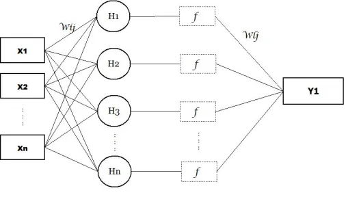
For a classic artificial neural network, its basic structure is shown as Figure. 1. Only one single hidden layer is deployed and the number of neurons is usually playing a key role in performance of every different algorithm.

Fig. 1: Classic ANN Diagram

In Figure. 1, {xi,yi} represents input and output layer units in this traditional model. For this type of feed-forward network, formulas between these three layers are shown below.

hi= n

X

1

Wij*xi-bi (1)

hi=f(βi∗hi) (2)

yi= n

X

1

Wlj*hj (3)

From these formulas, there is a bunch of parameters namely

{Wij,Wlj,hi,bi,βi,ε, f}. Wij shows the connection strength between the input layer unitsxi and the hidden layer unitshj. Accordingly Wlj shows the connection strength between the hidden layer unitshland the output layer unitsyj. Formula (1) shows how the input layer units impact the hidden layer units neurons. Every input layer units show its effect on these hidden layer neurons. And Formula (2) contains an activation function f which is considered as a reaction to these inputs. Actually these output of hidden layers neurons are defined by bi,βi,f. Back-propagation (BP) algorithm and support vector machine (SVM) methods are normally used in this ANN model.

In our design, we use this classic artificial neural network for our groundwater prediction model. Similar to our earlier work[15], Monte Carlo Algorithm substitutes classic algo-rithms such BP and SVM for parameter searching. It can be regarded as a computational algorithm based on repeating random sampling to approach an optimal result. While in [15] we have used this algorithm in classification problem, we can also adapt it to our prediction model. In our experiments it

EAI Endorsed Transactions on

Scalable Information Systems

shows powerful ability in time series learning not only in underground water prediction but also Smart Grid prediction. In this paper we will focus on underground water prediction. Unlike that SVM searches support vector and the best fit kernel function for model, Monte Carlo Algorithm will conduct the general vector searching task and finally mapping data task, as much and precise as it can, into the model. As support vectors always demonstrate a good performance for its structure, once a suitable kernel function is found for the dataset, in this paper, Monte Carlo Algorithm is also deployed in a shallow network. With an acceptable time consumption, this structure could lead to a better prediction result.

In our original algorithm, all the parameters in this bunch,

{Wij,Wlj,hi,bi,βi,ε, f}, could be updated to suit its goal. In this paper, we simply fix parameters Wlj which is between hidden layer and output layer. The rest of these parameters, including {Wij,bi,βi,ε} could be updated for one parameter each time when the cost function leads to a better performance. We herein use a different cost funtion from [15] to approach the final result.

In this shallow model,WijandWljstand for two connected layers, including input layer and hidden layer, and hidden layer and output layer. bi represents the bias of each hidden layer units. The βi correspond to the transfer function coefficients.

εis a correcting unit for each parameters used in Monte Carlo Algorithm. In each iteration we updateεto other parameters, herein it is mainly about{Wij,bi,βi}. When usingεto adjust other parameters to fit data relationships, each time only one random paramter is selected and being tried to update. Only if the cost function gets a not-worse result should the parameter be updated. In other words, we accept this adjustment only when the cost function ∆ reduces or holds.

As shown below Formula (4) is the cost function ∆.

∆ = v u u t 1 n n X 1

(yi−yi0)2 (4)

A main procedure of this Monte Carlo Algorithm is pre-sented in detail below.

A. Initialization

Network requires an initial value to start working. Here we set these parameters Wij, Wlj, bi, βi, ε to random values within a fixed interval. These intervals are selected empirically and they are critical in our analysis.

B. Update parameters

Choose one group of the parameters from{Wij,Wlj,bi,βi}. Model randomly chooses one parameter from this bunch, adjusts it with the ε and calculates yi and ∆. If ∆ is not becoming worse, then we accept this change and move on to next round. This step stops after a Monte Carlo Steps.

C. Repeat Monte Carlo Steps on other parameters

Change to other types of parameters from{Wij,Wlj,bi,βi} after a Monte Carlo Steps.

D. Stop training

Repeatedly train this shallow neural network via B and C steps and stop when either a critical time runs outt ≥t0 or cost function∆≤∆0.

In our work, this shallow neural network is applied to underground water time series prediction problem. The orig-inal underground water data has been obtained for decades [16, 17]. In [15] we used a modified cost function instead of square root value to overcome the over-fitting problem. In this paper, square root as shown in Formula (4) is used to approximate the best prediction model for underground water. Cost function is the key factor in Monte Carlo Algorithm. It varies a lot to fit different situations for its practical results taking into the consideration of time consumption and accuracy. We have shown a powerful ability of this Monte Carlo Algorithm to fit different situations in our studies in different applications. In next section we will focus on datasets and its experiments.

IV. DATASETS ANDEXPERIMENTS

Even though data is collected in a reliable method, there is a data sparsity problem due to inadequate measuring methods in the past decades. Hence we reconstruct these data in a reasonable way.

There is not any pre-processing with these data and its inner noise, which is inevitably existing in these data and is however overcome by our Monte Carlo Algorithms. We show our result without any pre-processing. And the local field theory demonstrate that noise could be used to facilitate model’s learning and optimize its result as [18] and [19] had illustrated. Therefore via curating a dataset from the original data, we get a model containing enough units.

A. Dataset

In previous decades, exactly 1986-2008, the underground water data of 26 related spots had been collected. They are all located in Heihe River basin, which means these 26 related spots data could have some internal relationship. Our curated data comes from a sub group of these 26 observa-tion spots, namely Banqiaodongliu spot, Pingchuangongcheng spot, Shandanqiao spot, Wangqizha spot, Xiaohe spot, Xingou spot, Yaruanzhangwan spot, Zhangyenongchang spot and Sha-jingzi spot.

In this paper, we build a dataset including eight observation feature spots and one observation label spot for a time series prediction. Overall noises exist in this dataset resulted from its data collection technology. However we still input them directly into this shallow neural network for training. It is a bit different from [15]. The cost function used in this paper and output layer setting have been changed accordingly.

B. Model

As shown in Figure. 2, this is the original shallow neural network with 8 units input, 1 units output and 200/500 hidden neural units.

EAI Endorsed Transactions on

Scalable Information Systems

Fig. 2: Original Neural Network

C. Parameters Value Interval

It is an empirical issue for selecting suitable parameters value interval. And in our paper,{Wij,bi,βi}are chosen to be positively updated for a better cost function whileWljremains the same once it is decided at initialization stage.

Wlj is fixed into two groups of experiments, for {+0.10, -0.10}and{+0.01, -0.01}. Also through the change of neural transfer function, we have modified hidden neural units to observe its performance.

D. Procedure

In this subsection, the main procedure of our Monte Carlo Algorithm (see Algorithm 1) is presented.

E. Experiments

Experiments are conducted under four different settings but all achieve a good performance in their results. In our experiments, we deploy two different transfer neural functions asx2_{+xandx. Below we will show the results with different} settings.

As a baseline work, we chose Back Propagation algorithm as our comparison method, since most of literatures [13, 14] used BP as their method. As shown in Fig. (3) was the training result and Fig. (4) was the test result. The MSE result of the test dataset was 0.56, while in our model it was 0.113.

Fig. 3: Training on Back Propagation algorithm

Algorithm 1 Monte Carlo algorithm

init supervised model: Calculate Output Layer statusyi with a pre-setting values of all parameters.

Calculate Cost Function: Calculate Cost Function value∆1.

1: if ∆1 ≥∆0 then

2: ifstep < M onteCarloStep then 3: ε= random(+ε0,-ε0);

4: Select a randomWij from Wij matrix; 5: Wij = Wij +ε;

6: update Output Layer statusyi; 7: Calculate Cost Function value∆; 8: while ∆ ≤∆0 :

9: updateWij; 10: update∆1; 11: end if 12:

13: ifstep < M onteCarloStep then 14: ε= random(+ε0,-ε0);

15: Select a randomβi fromβi matrix; 16: βi = βi + ε;

17: update Output Layer statusyi; 18: Calculate Cost Function value∆; 19: while ∆ ≤∆0 :

20: updateβi; 21: update∆1; 22: end if 23:

24: ifstep < M onteCarloStep then 25: ε= random(+ε0,-ε0);

26: Select a randomWij from Wij matrix; 27: bi = bi + ε;

28: update Output Layer statusyi; 29: Calculate Cost Function value∆; 30: while ∆ ≤∆0 :

31: updatebi; 32: update∆1; 33: end if 34: end if

Fig. 4: Test on Back Propagation algorithm

EAI Endorsed Transactions on

Scalable Information Systems

As shown in Fig. (5) and (6), a 200 hidden neural units layer was allocated for our first experiment. In this network, ax2_{+xtransfer function was used and also the value ofW}

lj is{+0.1, -0.1}. It delivered a good performance of prediction.

Fig. 5: Training under 200 hidden units andx2_+xfunction

Fig. 6: Result under 200 hidden units andx2_+xfunction

In the next, we slightly changed the parameter of Wlj from {+0.1, -0.1} to {+0.01, -0.01}, the results showed an almost same result as we can tell from Fig. (7) and (8). It demonstrated that under Monte Carlo Algorithm category, this shallow neural network had a better learning and fitting ability for understanding the data. The high scalability could be obtained via a bunch of parametersWij, bi, βi, εeven when Wlj is fixed.

Fig. 7: Training under 200 hidden units andx2+xfunction

Fig. 8: Result under 200 hidden units andx2+xfunction

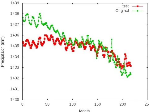
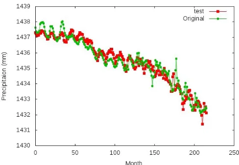
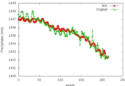
Fig. (9) and (10) demonstrated a better performance for our prediction in the case when we changed the transfer function fromx2_{+xtox. The trends and values in our test have shown} a better result under the construction of x transfer neural function. Furthermore, we also tried to configure a different size of hidden neural units. As shown in Fig. (11) and (12), the x transfer neural function got a better ability to fit data regardless of the hidden neural units size. In our previous test wherex2_{+xset as the transfer neural function, the best result} came from 200 hidden neural units.

From Fig. (9) and (10), a suitable transfer neural function achieved a even better and stable result with 200 and 500 hidden neural units. It showed that searching for general vectors in this shallow neural network was much easier with the deployment of Monte Carlo Algorithm. But for its perfor-mance, it would strongly depend on its neural network and cost function for a positive updating process.

EAI Endorsed Transactions on

Scalable Information Systems

Fig. 9: Training under 200 hidden units andxfunction

Fig. 10: Result under 200 hidden units andxfunction

Fig. 11: Training under 500 hidden units and xfunction

Fig. 12: Result under 500 hidden units and xfunction

V. CONCLUSION

Tackling water prediction problem nowadays is more important for a proper regional development strategy, especially in the arid Heihe River basin. In this paper, we have curated a dataset from two decades of collected data. A consideration of area related relationship is important in this paper. We tried to figure out the relationship between these nine observation spots selected out of the whole 26 spots. The Monte Carlo Algorithm [15] is an efficient approach as shown in our paper and we also discussed the internal settings and structure of the deployed shallow neural network.

The baseline work in our paper is Back Propagation algorithm. We achieve a better result than BP while in BP the MSE result is 0.56 and in our model it is 0.113. The results is promising in dealing with the difficulties in such problem.

In the future work, expanding this method to other data curated not only from our own data but also other researchers’ available data is under consideration. Also introducing bio-inspired algorithm [20] to facilitate the training speed and performance of Monte Carlo algorithm. And a comparison between our approach and the state of art of deep learning methods will also be undertaken.

ACKNOWLEDGMENT

This work is supported by a scholarship from the China Scholarship Council while the second author pursues his PhD degree in University of Wollongong. This work was supported by National Natural Science Foundation of China under Grant No. 61402210 and 60973137, Program for New Century Excellent Talents in University under Grant No. NCET-12-0250, ”Strategic Priority Research Program” of the Chinese Academy of Sciences with Grant No. XDA03030100, Gansu Sci.&Tech. Program under Grant No. 1104GKCA049, 1204GKCA061 and 1304GKCA018. The Fundamental Research Funds for the Central Universities under Grant No. 2014-49, 2013-k05, 2013-43, 2013-44, 2014-235 and

lzujbky-EAI Endorsed Transactions on

Scalable Information Systems

Faculty Award, China. This work is also facilitated by the help of University of Wollongong’s University Internationalisation Committed’s UIC Linkage program and Global Challenge Program’s Travel Fund.

REFERENCES

[1] T. Kuremoto, S. Kimura, K. Kobayashi, and M. Obayashi, “Time series forecasting using a deep belief network with restricted Boltzmann machines,”

Neurocomputing, vol. 137, pp. 47–56, 2014.

[2] H. Wang, Y. Zhang, and J. Cao, “Access control man-agement for ubiquitous computing,” Future Generation Computer Systems, vol. 24, no. 8, pp. 870–878, 2008. [3] L. Wang, J. Shen, and J. Yong, “A survey on bio-inspired

algorithms for web service composition,” in Computer Supported Cooperative Work in Design (CSCWD), 2012 IEEE 16th International Conference on. IEEE, 2012, pp. 569–574.

[4] M. Li, X. Sun, H. Wang, Y. Zhang, and J. Zhang, “Privacy-aware access control with trust management in web service,”World Wide Web, vol. 14, no. 4, pp. 407– 430, 2011.

[5] I. N. Daliakopoulos, P. Coulibaly, and I. K. Tsanis, “Groundwater level forecasting using artificial neural networks,” J. Hydrol., vol. 309, no. 1-4, pp. 229–240, 2005.

[6] L. W. Mays, “Groundwater Resources Sustainability: Past, Present, and Future,”Water Resour. Manag., vol. 27, no. 13, pp. 4409–4424, 2013.

[7] D. K. Todd,Ground water hydrology. New York : Wiley, 1959, includes bibliography.

[8] S. Mohanty, M. K. Jha, A. Kumar, and K. P. Sudheer, “Artificial neural network modeling for groundwater level forecasting in a river island of eastern India,” Water Resour. Manag., vol. 24, no. 9, pp. 1845–1865, 2010. [9] C. Hamzac¸ebi, “Improving artificial neural networks’

performance in seasonal time series forecasting,”Inf. Sci. (Ny)., vol. 178, no. 23, pp. 4550–4559, 2008.

vol. 50, pp. 159–175, 2003.

[11] E. Coppola Jr., M. Poulton, E. Charles, J. Dustman, and F. Szidarovszky, “Application of Artificial Neural Net-works to Complex Groundwater Management Problems,”

Nat. Resour. Res., vol. 12, no. 4, pp. 303–320, 2003. [12] M. Baker and R. Patil, “Universal approximation theorem

for interval neural networks,”Reliable Computing, vol. 4, no. 3, pp. 235–239, 1998.

[13] R. Bustami, N. Bessaih, C. Bong, and S. Suhaili, “Ar-tificial neural network for precipitation and water level predictions of bedup river,”IAENG International journal of computer science, vol. 34, no. 2, pp. 228–233, 2007. [14] S. Rani and F. Parekh, “Predicting reservoir water level using artificial neural network,”International Journal of Innovative Research in Science, Engineering and Tech-nology, vol. 3, pp. 14 489–14 496, 2014.

[15] H. Chen, H. Zhao, J. Shen, R. Zhou, and Q. Zhou, “Supervised machine learning model for high dimen-sional gene data in colon cancer detection,” inBig Data (BigData Congress), 2015 IEEE International Congress on, June 2015, pp. 134–141.

[16] X. Wu, J. Zhou, H. Wang, Y. Li, and B. Zhong, “Eval-uation of irrigation water use efficiency using remote sensing in the middle reach of the heihe river, in the semi-arid northwestern china,” Hydrological Processes, vol. 29, no. 9, pp. 2243–2257, 2015.

[17] X. H. Wen, Y. Q. Wu, L. J. E. Lee, J. P. Su, and J. Wu, “Groundwater flow modeling in the Zhangye Basin, Northwestern China,”Environ. Geol., vol. 53, pp. 77–84, 2007.

[18] H. Zhao and T. Jin, “A global algorithm for training mul-tilayer neural networks,” arXiv preprint physics, 2006. [19] H. Zhao, “Designing asymmetric neural networks with

associative memory,”Physical Review E, vol. 70, no. 6, 2004.

[20] L. Wang, J. Shen, J. Luo, and F. Dong, “An improved genetic algorithm for cost-effective data-intensive ser-vice composition,” in Semantics, Knowledge and Grids (SKG), 2013 Ninth International Conference on. IEEE, 2013, pp. 105–112.

EAI Endorsed Transactions on

Scalable Information Systems