U
U
S
S
I
I
N
N
G
G
A
A
R
R
E
E
M
M
O
O
T
T
E
E
L
L
Y
Y
C
C
O
O
N
N
T
T
R
R
O
O
L
L
L
L
E
E
D
D
P
P
L
L
A
A
T
T
F
F
O
O
R
R
M
M
T
T
O
O
A
A
C
C
Q
Q
U
U
I
I
R
R
E
E
L
L
O
O
W
W
-
-
A
A
L
L
T
T
I
I
T
T
U
U
D
D
E
E
I
I
M
M
A
A
G
G
E
E
R
R
Y
Y
F
F
O
O
R
R
G
G
R
R
A
A
I
I
N
N
C
C
R
R
O
O
P
P
M
M
A
A
P
P
P
P
I
I
N
N
G
G
A Dissertation submitted by
Troy Arnold Jensen
B.Eng (DDIAE)
M.Eng (USQ)
For the award
D
Do
oc
c
t
t
or
o
r
o
of
f
P
Ph
hi
il
lo
os
so
op
ph
hy
y
Dedication
Agricultural crops exhibit within-field spatial variation. This variation partly results from relevant bio-physical and environmental factors that influence the crop during the growing season. The plant integrates the effects of nutrition, water, pests and disease, and displays the results in the foliage. Remote sensing techniques allow the foliage to be monitored and the crop status to be assessed.
While the use of conventional remote sensing systems has found many applications in agriculture, it is constrained by a number of issues and problems related to spatial resolution, repeat cycle, minimum area acquired, timeliness of data, etc. Thus, this research explores the potential of developing and assessing low-cost sensing technologies to overcome these limitations. The specific objectives were to: a) identify, evaluate, and analyse the different options for a low-cost low-altitude (LCLA) remote sensing system that has potential for precision agriculture, b) develop a LCLA remote sensing system that is appropriate for use in mapping selected crop attributes (i.e. grain protein, yield, maturity and crop type), and c) evaluate the accuracy of classification and prediction of the cereal crop attributes.
A low-cost sensor system was developed that incorporated two consumer digital still cameras. One camera captured the colour portion of the spectrum, while the other one (with the addition of a band-pass filter) captured the near infrared light. Both cameras were modified to be remotely triggered and externally powered. This sensor arrangement utilised 1.0 megapixel cameras in the earlier investigations and then 5.0 megapixel cameras in most recent missions. The sensors were equally well suited to mounting on a remotely controlled aircraft or suspended beneath a helium balloon.
classifications.
The results showed that low-cost low-altitude remote sensing systems (incorporating consumer digital cameras with helium balloons or remotely controlled aircraft) have great capacity to quantify variability in cereal grain crops. Excellent relationships were found between the ‘at-harvest’ yield (R2=0.902) and protein content (R2=0.660) of wheat using a single image recorded at flowering. Partial least squares regression, using the cross-validated approach, produced a stronger relationship with a prediction accuracy of 94.2% for yield and 88.5% for protein. This relationship exceeded all other studies reported in the literature.
The same LCLA system has also accurately discriminated (using statistical methods) between: a) different nutrition levels in a wheat crop with 75.6% of the cases correctly classified, and b) between different cereal grain species (with differing nutrition levels) with 86.3% accuracy. These classification accuracies are comparable with, or exceeding other more expensive and/or complicated methods. Attempting to discriminate using image analysis procedures, the pixel-based methods yielded an overall accuracy of 65.9% when classifying cereal grain crop species comprising of nine classes. When merged to six classes, the accuracy improved to 82.1%. Using an
object-orientated approach has improved the overall accuracy to 81.0% for the nine-category classification. This study also demonstrated LCLA’s ability to assess the various growth stages of a barley crop prior to maturity with 83.5% of cases
correctly classified.
I certify that the ideas, experimental work, results, analyses, software and conclusions reported in this dissertation are entirely my own effort, except where otherwise acknowledged. I also certify that the work is original and has not been previously submitted for any other award, except where otherwise acknowledged.
_________________________ ________________
Signature of Candidate Date
ENSORSEMENT
_________________________ ________________
Signature of Supervisor Date
Published International Journal
Jensen, TA, Apan, A, Young, F & Zeller, LC 2007, 'Detecting the attributes of a wheat crop using digital imagery acquired from a low-altitude platform',
Computers and Electronics in Agriculture, vol. 59, no. 1-2, pp. 66-77.
Published Conference Proceedings
Hussain, A, Raine, SR, Henderson, CW & Jensen, TA 2008, 'Evaluation of a proximal vision data acquisition system for measuring spatial variability in lettuce growth', paper presented to Global Issues, Paddock Action - 14th Australian Agronomy Conference, Adelaide, Australia, 21-25 September 2008.
Jensen, TA, Apan, A, Young, F & Zeller, L 2005, 'Grain Crop Attributes Detected Using Digital Imagery Acquired from a Low-Altitude Helium balloon', paper presented to 5th European Conference on Precision Agriculture, Uppsala Sweden, 9-12 June 2005.
Jensen, TA 2004, 'Remote sensing – an innovative balloon platform', paper presented to 8th Annual Symposium on Precision Agriculture Research & Applications in Australasia, Sydney, Australia, 20 August 2004.
Jensen, TA, Apan, A, Young, F, Zeller, LC & Cleminson, K 2003, 'Assessing grain crop attributes using digital imagery acquired from a low-altitude remote controlled aircraft', paper presented to First Spatial Sciences Conference, Canberra, Australia, 22-27 September 2003.
Jensen, TA, Apan, A, Young, F & Zeller, LC 2002, 'Capturing of remotely sensed images to advance the use of yield maps and other spatial information to improve crop management and forecasting.' paper presented to 11th Australasian Remote Sensing and Photogrammetry Conference, Brisbane, Australia, 2-6 September 2002.
Popular Press
Alcorn, G 2004, 'The balloon goes up on crop monitoring', Australian Grain, vol. 14, no. 1, pp. 48-9.
I thank my principal supervisor Associate Professor Armando Apan for his infinite wisdom, direction and motivation throughout this work. My associate supervisor, Associate Professor Frank Young, also provided valuable comments and suggestions.
Les Zeller has provided friendship, motivation, electronic skills, assistance in data collection and was also a great sounding board for ideas.
Ken Cleminson provided advice on things remotely controlled and access to his planes, as well as flying them, during the early development stages of this project.
Dr. Wayne Strong expounded his infinite agronomic wisdom to me when I needed assistance.
Ross and Jordie Milne kindly provided access to their plane, as well as in flying the craft in the later stages of the project.
To the ARCAA team from QUT for the use of their autonomous UAV during the final testing of my concept, my thanks.
My appreciation to the now defunct DPI&F Precision Agriculture team for the access to datasets and funds for this work that ran in parallel to their GRDC-funded projects.
Abstract ... iii
Certification of Dissertation ... v
Publications Related to this Thesis ... vi
Acknowledgements ... vii
List of Figures ... x
List of Tables ... xvi
Abbreviations ... xiii
Chapter 1 Introduction ... 1
1.1 Background ... 1
1.2 Research Problem and its Significance ... 3
1.3 Research Objectives ... 3
1.4 Context, Scope and Delimitation of the Study ... 4
1.5 Organisation of the Thesis ... 6
Chapter 2 Literature Review: Precision Agriculture and Remote Sensing ... 9
2.1 Precision Agriculture ... 9
2.1.1 Definition and Components ... 11
2.1.2 Purpose and Benefits ... 18
2.1.3 Limitations and Opportunities of Precision Agriculture ... 18
2.2 Remote Sensing ... 19
2.2.1 Basic Concepts ... 19
2.2.2 Methods of Remote Sensing ... 23
2.2.3 Problems and Limitations of Using Existing Remote Sensing Systems in Precision Agriculture ... 32
2.2.4 Technologies for use in a Low-Cost Low-Altitude Remote Sensing System ... 33
2.3 Summary ... 37
Chapter 3 Preliminary Evaluation and Assessment of Sensor and Platform Systems ... 38
3.1 Potential Systems ... 38
3.1.1 Platform ... 38
3.1.2 Sensor System ... 43
3.2 Requirements for a LCLA System for Precision Agriculture ... 44
3.2.1 Deployment Considerations ... 44
3.2.2 Crop Considerations ... 45
3.2.3 Legislative Requirements ... 45
3.2.4 Costs ... 47
3.3 Preliminary Deployment and Assessment of a Sensor and Platform System ... 48
3.3.1 Platform System ... 48
3.3.2 Sensor System ... 51
3.4 Conclusions ... 74
Chapter 4 Developing a LCLA Remote Sensing System ... 76
4.1 The Case for the 2-Camera System ... 76
4.1.1 Justification for Adoption ... 76
4.1.2 Specifications for the Improved System ... 77
4.2.2 1.0 Megapixel Digital Camera Sensor System... 81
4.2.3 5.0 Megapixel Digital Camera Sensor System... 94
4.2.4 Tasking and Deployment... 103
4.2.5 Costings for the LCLA System ... 105
4.3 Conclusions ... 106
Chapter 5 Crop Mapping Methods using the LCLA System ... 108
5.1 Introduction ... 108
5.2 Grain Yield and Protein Mapping ... 110
5.2.1 Study Area ... 110
5.2.2 System Deployment ... 116
5.2.3 Image Processing and Analysis ... 123
5.2.4 Statistical Analysis ... 132
5.3 Crop Type Discrimination and Mapping ... 134
5.3.1 Study Area ... 134
5.3.2 System Deployment ... 135
5.3.3 Pixel-Based Image Processing and Analysis ... 143
5.3.4 Object Orientated Image Classification ... 153
5.4 Further Refinement ... 156
5.4.1 Crop Maturity Mapping ... 156
5.4.2 Autopilot Evaluation ... 164
5.5 Conclusions ... 170
Chapter 6 Performance of the LCLA system for Crop Mapping ... 171
6.1 Introduction ... 171
6.2 Grain Yield and Protein Mapping ... 171
6.2.1 The Yield-Protein Relationship ... 172
6.2.2 Analysis of Variance ... 172
6.2.3 Correlation Analysis ... 173
6.2.4 Discriminant Function Analysis ... 180
6.2.5 Partial Least Squares Regression ... 184
6.3 Crop Type Discrimination and Mapping ... 191
6.3.1 Discriminant Function Analysis ... 191
6.3.2 Pixel-Based Image Classification ... 201
6.3.3 Object-Oriented Image Classification ... 228
6.4 Further Refinements ... 236
6.4.1 Crop Maturity Mapping ... 236
6.4.2 Autopilot Evaluation ... 247
6.5 Synthesis of Findings ... 253
6.5.1 Sensor ... 253
6.5.2 Platform ... 254
6.6 Conclusions ... 254
Chapter 7 Conclusions and Recommendations ... 256
7.1 Introduction ... 256
7.2 Summary of Findings ... 256
7.3 Conclusions ... 259
7.4 Recommendations for Future Work ... 261
References ... 262
Figures Page
1.1 The schematic layout of this thesis. ... 8
2.1 The precision agriculture wheel (McBratney & Whelan 2001). ...13
2.2 A simplified cross-section of the human eye (Mather 2004). ... 20
2.3 Trichromatic theory of colour vision (Jensen 2007). ...20
2.4 The visible portion and other components of the electromagnetic spectrum (Jensen 2007). ...21
2.5 Spectral reflectance curves for natural features in the range 400–2500 nm (Geoimage 2005). ... 22
2.6 Bayer filter pattern. ... 36
3.1 The ‘Magic’ UAV and the 36 MHz radio control gear used at UQG (Mission #4). ...50
3.2 The components of the 2.4 GHz surveillance video system–transmitter (left), camera (middle) and receiver (right). ...52
3.3 The analogue video stream is intercepted by the video receiver and recorded on the digital video recorder. The 12 V battery is powering the video receiver. ...52
3.4 The ‘Zephyr’ UAV with wing removed (left), radio control gear (middle) and starter box containing fuel and battery charger (right) prior to deployment. ...53
3.5 The ‘Zephyr’ UAV showing the hole for the mini video camera in the underside of the fuselage (between the two white strips). ... 54
3.6 A frame-grabbed image showing a car driving along a dual carriage-way (note the banding in the image) acquired during Mission #1. ...55
3.7 The spectral response for the Kodak KAI-0340 (Kodak 2008) showing the response for the monochrome sensor in black and that of the blue/green/red sensors in the corresponding colours. ...56
3.8 Transmittance of the Hoya R72 filter for the various wavelengths of light. ...57
3.9 An NIR image collected with the video camera-frame grabber setup on Mission #1 (note the bright signature of the row of trees through the centre of the image). ...57
3.10 A 35 mm instamatic camera, installed in a mounting frame and utilising a servo to depress the shutter button, that was used to take images from a UAV. ...59
3.11 The Kodak DC3200 digital camera. ... 60
3.12 The single DC3200 camera attached to the underside of the 1.4 m wingspan ‘Magic’ UAV. ...61
3.13 The DC3200 mounted underneath the UAV (note the rotary servo to depress the shutter release button). ... 63
3.14 An image capture on Mission #3 showing the layout of the land. ...63
3.15 More detailed information captured during Mission #3. ...64
3.16 A low-level image collected during Mission #3. ...65
location of the car and points A & B both images). ...67
3.20 Image of tree with Hoya R72 filter (left) and in normal mode (right), (Mission #5). ...69
3.21 The camera settings when taking the images in Figure 3.20. ...70
3.22 Spectral response with and without IR cut-out (Vaytek 2003) ...71
3.23 The DC 3200 pulled apart showing the 'blue' IR cut-out filter. ...72
3.24 Testing the output of the 29 MHz 2 channel radio control transmitter. ...73
3.25 The change in the output signal from the receiver when the throttle / rudder stick was moved. The output was noisy, making it difficult to measure. ...74
4.1 The 2-camera sensor system. ...82
4.2 The image pair, with the NIR (top) and CIR image (bottom), taken out of the car window at 60 kph. ...84
4.3 The sensor installed under the ‘Hannibal’ UAV at the TARMAC test, 12 June 2003...85
4.4 Simultaneous images captured from a UAV, utilising a Hoya R72 filter (top) and the CIR (bottom). ...86
4.5 The sensor installed underneath the helium balloon, 14 June 2003. ...88
4.6 The colour (top) and NIR (bottom) image collected from the helium balloon at Argyle, 14 June 2003. ...89
4.7 The 2-camera sensor installed under the 'Hannibal' UAV during the ‘Argyle’ mission, 1 August 2003. ...90
4.8 The 'Hannibal' UAV ready for take-off, 1 August 2003. ...91
4.9 The 2-camera sensor with camera-status detection. ...93
4.10 The Kodak CX7525 digital zoom camera. ...94
4.11 The CX7525 that has been modified to increase sensitivity to near-infrared light and to enable electronic triggering. ...96
4.12 The 2-camera sensor utilising the CX7525 cameras (top view). ...98
4.13 The underside view of the 2-camera sensor and the radio control transmitter. ...99
4.14 The CX7525 2-camera sensor installed in the ‘Milne’ UAV. ...100
4.15 The ‘Milne’ UAV being prepared for takeoff, 20 September 2005. ...100
4.16 The near-infrared image collected on the ‘Daybreak’ mission, 20 September 2005. ... 101
4.17 The matching colour image for Figure 4.16. ...102
5.1 The sequences for digital image analysis adopted in this research. 109 5.2 Location of the Colonsay trial in the Central Darling Downs region of Queensland. ...110
5.3 Schematic layout of 'Colonsay' site for 2003. ...112
5.4 Example of a plot with low nutrition levels (left) and high nutrition levels (right). ...113
5.7 The range of plant available water contents for the various soil depths across the range of nitrogen treatment plots, immediately prior to planting
in 2003...115
5.8 The range of available nitrogen for the various soil depths across the range of nitrogen treatment plots, immediately prior to planting in 2003. ...116
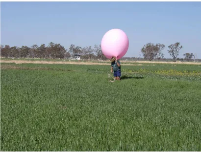
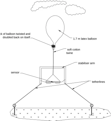
5.9 Tieing-off the inflated latex balloon with soft cotton string. ... 117
5.10 A schematic representation of the sensor as deployed on 2 September 2003. ...118
5.11 Preparing for sensor deployment at 'Colonsay'. ...119
5.12 The sensor is airborne. ...119
5.13 Colour image of the NW corner of the trial site. ...120
5.14 The NIR image that matches with the colour image shown in Figure 5.13. ...120
5.15 A schematic representation of the sensor as deployed on 14 October 2003. ...122
5.16 The balloon attached to the stabilising frame with the sensor suspended underneath prior to deployment at a football stadium. ...123
5.17 The colour image that was further processed. ...124
5.18 The ground control points used to geo-reference the image. ...125
5.19 Ground control points chosen to register the colour to the NIR image. ...127
5.20 Selecting the areas of interest for the whole treatment and the ‘5x5 kernel’ study. ...128
5.21 Box-plots of the digital numbers for the various bands, selected using the ‘5 x 5’ kernel (left) and whole plot (right) AOIs (subplots 45 and 46). ...129
5.22 Selecting the area of interests (AOIs) for each of the plots (note the two pixel margin around each plot). ...130
5.23 Box-plot of the digital numbers for all six bands for plot 41 (0 kg/ha N applied – left) and plot 51 (40 kg/ha N applied – right). ...131
5.24 Box-plot of the digital numbers for all six bands for plot 57 (80 kg/ha N applied – left) and plot 43 (120 kg/ha N applied – right). ... 131
5.25 Location of the ‘Dunkerry South’ trial, near Nindigully, in south-western Queensland. ...134
5.26 Schematic representation of the 'Dunkerry South' farming systems trial showing the treatments and plot layout. ...136
5.27 The sensor being retrieved at Nindigully (note the breeze blowing the balloon)...137
5.28 A schematic representation of the sensor as deployed, 13 September 2004. ...138
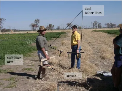
5.29 The sensor ready to be deployed at Nindigully, with two tether-lines for increased stability. ...139
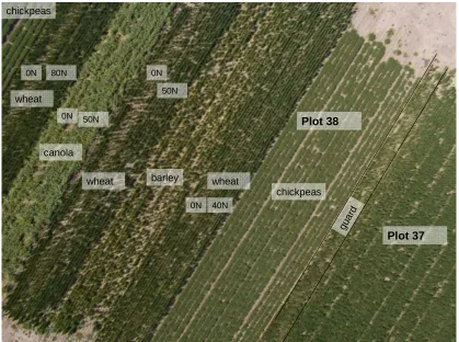
5.30 An image captured on the first mission covering adjacent plots showing a range of species present, as captured by the LCLA remote sensing system. ...140
5.34 Selecting AOIs for each of the subplots within plot 38. ...145
5.35 Box-plots for wheat 40 N (left) and chickpeas (right) for the 6 bands. ...145
5.36 Average digital number values for the sub-plots within plot 38 for the various bands. ...146
5.37 Box-plots of the pixel values for the polyline positioned down the centre of the row for each of the six bands for wheat 40 N (left) and chickpeas (right). ...148
5.38 Plot 41 and surrounding plots showing different species present...149
5.39 The layer stacking procedure of the 2 images in the analysis software. ...150
5.40 A close-up of the polyline area-of-interest for the wheat 50 N plot. ...152
5.41 Signature editor showing the 12 classes. ...152
5.42 Segmentation parameters used in the object-oriented approach (showing the 30 scale as an example) ...154
5.43 Classes adopted in the classification ... 155
5.44 The location of the trial site at ‘Lundavra’ in southern Queensland. ...157
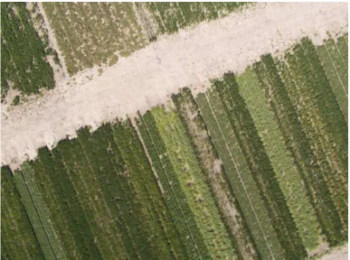
5.45 Conventional aerial image taken of the wheat (top) and barley (bottom) variety trial site at ‘Lundavra’, October 2005. The area indicated in red box is the area analysed. ...158
5.46 Schematic layout of the barley variety trial at ‘Lundavra’ showing the area analysed in the red box. ...159
5.47 Looking into the field towards the wheat trial area (note the advanced stage of the crop). ...160
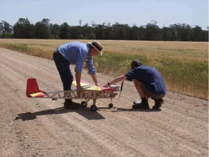
5.48 Preparing the ‘Milne’ UAV for deployment at ‘Lundavra’. ... 161
5.49 Some of the variability evident in the wheat trial area. ...161
5.50 Selecting the AOIs from the individual plots in the investigated area covered by the red box in Figure 5.45. ...163
5.51 Location of the Watts Bridge Memorial Airfield. ...165
5.52 The QUT UAV read for take-off. ...166
5.53 The avionics installed in the QUT UAV. ...167
5.54 The pod opened to remove the SD cards from the LCLA sensors. ...167
5.55 The ground control station software showing the path and the flight details of the UAV being monitored in the autopilot flight software (note the waypoints in pink). ...169
6.1 The relationship between yield and protein for the ‘Colonsay’ dataset. ...172
6.2 Scatterplot of the 6 bands and yield / protein...173
6.3 Scatterplot of the derived indices and yield / protein. ...174
6.4 The relationship between yield and digital number for the NIRR band (left) and DVI (right) for the various N application rates. ...176
6.5 The relationship between protein and digital number for the NIRR band (left) and from DVI (right) for the various N application rates. ...178
the PLS regression model involving vegetation index values. ...185
6.9 Plot of predicted grain protein values vs. measured grain protein values from the PLS regression model involving raw imagery values. ...186
6.10 Plot of predicted grain protein values vs. measured grain protein values from the PLS regression model involving vegetation index values. ...186
6.11 Regression coefficients for the cross-calibrated prediction model involving grain yield and raw imagery values. ... 188
6.12 Regression coefficients for the cross-calibrated prediction model involving grain yield and vegetation index values. ...189
6.13 Regression coefficients for the cross-calibrated prediction model involving grain protein and raw imagery values. ... 190
6.14 Regression coefficients for the cross-calibrated prediction model involving grain protein and vegetation index values. ...190
6.15 The canonical plot for the various species and fertiliser rates. ...194
6.16 The canonical plot for the various species and fertiliser rates. ...198
6.17 The band histogram information for the training sets for the chickpea signature...202
6.18 The band histogram information for the training sets for the wheat 50N signature...202
6.19 The key to the colours used in the histograms and the classification. ...203
6.20 The histograms for the merged signatures of the non-cropped areas ...203
6.21 The histograms for the merged signatures of the cropped areas ...204
6.22 The feature space plot for the 12 classes. ...205
6.23 The alarm mask function of ERDAS Imagine ...209
6.24 The classified image using the 12 classes. ...211
6.25 Performing an accuracy assessment on the image ...212
6.26 The colours chosen and the pixel count for the 9 classes. ... 217
6.27 Histograms for the 9 classes ...219
6.28 Feature space plot for the 9 classes ... 219
6.29 The classification using 9 classes. ...220
6.30 The 6 class signatures. ...222
6.31 The histograms for the 6 classes. ...223
6.32 The area when classified using 6 classes. ...223
6.33 The histograms for the 4 classes. ...226
6.34 The area when classified using 4 classes. ...226
6.35 Objects created after image segmentation at various scales: (a) 30 scale, (b) 50 scale, (c) 80 scale, and (d) 100 scale. ...228
6.36 Classified image from the 30-scale image segmentation ... 231
6.37 Classified image from the 50-scale image segmentation ... 232
6.38 Classified image from the 80-scale image segmentation ... 233
stages. ...242
6.42 The frequency and distribution for the 3 principal growth stage classes. ...245
6.43 The flight paths and target positioning, Watts Bridge 5 March 2008. ...248
6.44 Image 100_4814 taken at 3:27:44 pm. ...249
6.45 Image 100_4815 taken just over 3min after image 100_4814 (shown in Figure 6.44). ...249
Table Page
2.1 Imaging properties of some remote sensing satellites ...24
2.2 Potential vegetation indices that can be calculated with multispectral remotely sensed data ...31
3.1 Comparison of various UAV platform types to perform LCLA remote sensing applications in agriculture (☼☼☼☼ indicates high compliance, ☼ indicates no or low compliance) ... 40
3.2 Some applications of UAVs in remote sensing ...41
3.3 The missions undertaken as part of the preliminary investigation. ...48
3.4 Black and white video camera specifications. ...51
3.5 Specifications and computer requirements for Studio DV Version 7. ...55
3.6 The specifications of the Kodak DC3200 digital still camera. ...61
3.7 The specifications of the Canon PowerShot G2. ...68
4.1 Missions with the LCLA remote sensing system ...78
4.2 The specifications for the Kodak CX7525 digital camera. ... 95
4.3 Comparison between the DC3200 and CX7525 digital cameras...96
4.4 Deployment checklist for completion before each mission. ...104
5.1 The band information for the stacked image. ...150
5.2 Explanation of the growth stages describing the barley crop based on Zadok et al. (1974). ...164
6.1 The analysis of variance (ANOVA) conducted to determine statistical differences between the classes. ...173
6.2 Correlations between yield / protein and the 6 bands and 5 indices. ...175
6.3 Tests of equality of group means. ...180
6.4 Pooled within-group matrices. ...181
6.5 Summary of canonical discriminant functions (Eignenvalues (top) and Wilks’ lambda (bottom)). ...181
6.6 The structure matrix. ...182
6.7 Prediction accuracy of fertiliser treatment classification using discriminant analysis. ...183
6.8 PLS regression results of imagery values and yield and protein ...187
6.9 Tests of equality of group means ...192
6.10 Pooled within-group matrices ...192
6.11 Summary of canonical discriminant functions (Eignenvalues (top) and Wilks’ lambda (bottom)) ...193
6.12 The structure matrix. ...193
6.13 Classification results for the n=50 case study. ...195
6.14 Tests of equality of group means ...196
Wilks’ lambda bottom). ...197
6.17 The structure matrix. ...198
6.18 Classification results for the n=80 case study. ...200
6.19 Contingency matrix for the 12 classes. ...207
6.20 Transformed divergence for the 12 classes. ...209
6.21 The error matrix for the 12 class accuracy assessment. ... 213
6.22 The accuracy totals for the 12 class classification. ...215
6.23 Kappa statistics for the 12 class classification ...216
6.24 The contingency matrix for the 9 classes. ...218
6.25 The accuracy totals including kappa statistics for the 9 class classification. ...221
6.26 The contingency matrix for the 6 classes ...222
6.27 The accuracy totals including kappa statistics for the 6 class classification. ...224
6.28 The contingency matrix for the 4 classes. ...225
6.29 The accuracy totals including kappa statistics for the 4 class classification. ...227
6.30 Results of image segmentation and feature optimisation ... 229
6.31. Accuracy of images classified from the object-oriented approach ...235
6.32 Tests of equality of group means ...237
6.33 Pooled within-group matrices ...238
6.34 Summary of canonical discriminant functions (Eignenvalues top and Wilks’ lambda bottom). ...238
6.35 The structure matrix ...239
6.36 The classification result for the 14 Zadoks class study. ... 240
6.37 The Zadoks range for the grouped secondary growth stages ...242
6.38 The classification accuracy for the grouped secondary growth stages. 244 6.39 The Zadoks range of the 3 principal growth stage classes. ...245
6.40 The classification results for the 3 principal growth stages. ...246
6.41 The classification results for the primary growth stages. ... 246
AGL ... Above ground level
AMSA ... Australian Maritime Safety Authority ANOVA ... Analysis of variance
AOI ... Area-of-interest
ARCAA ... Australian Research Centre for Aerospace Automation
ASTER ... Advanced Spaceborne Thermal Emission and Reflectance Radiometer B ... Blue
BSD ... Best separation distance CASA ... Civil Aviation Safety Authority CCD ... Charged couple device CF ... CompactFlash
CIR ... Colour infrared
CMOS ... Complementary metal–oxide semiconductor DA ... Discriminant function analysis
DAS ... Days after sowing DC ... Direct current DGPS ... Differential GPS DN ... Digital number
DPI&F ... Department of Primary Industries and Fisheries (Queensland) DVI ... Difference Vegetation Index
G ... Green
GCP ... Ground control point
GIS ... Geographic information system GLCM ... Grey level co-occurrence matrix
GNDVI ... Green Normalised Difference Vegetation Index GPS ... Global positioning system
GRDC ... Grains Research and Development Corporation JPEG ... Joint Photographic Experts Group
LCLA ... Low-cost low-altitude LED ... Light emitting diode ML ... Maximum likelihood
NASA ... National Aeronautics and Space Administration NDVI ... Normalised Difference Vegetation Index NiMH ... Nickel-metal hydride
NIR ... Near infrared
PA ... Precision agriculture
PCI ... Peripheral component interconnect
PCMCIA ... Personal Computer Memory Card International Association PLS ... Partial least squares
PPR ... Plant pigment ratio
PSRI ... Plant Senescence Vegetation Index QUT ... Queensland University of Technology R ... Red
RCA ... Remotely controlled aircraft RGB ... Red-green-blue
RMS ... Root mean squared
RMSEP ... Root mean squared error of prediction RTK ... Real-time kinematic
RVI ... Red Ratio Vegetation Index SIPI ... Structure insensitive pigment index SLR ... Single lens reflex
SSCM ... Site-specific crop management
TARMAC ... Toowoomba Amateur Radio Model Club TM ... Thematic mapper
UAV ... Unmanned aerial vehicle
UQG ... University of Queensland Gatton US ... United States
USQ ... University of Southern Queensland UV ... Ultra violet
Introduction
1.1 Background
The ability to measure yield (tonnes / hectare), and more recently the quality (% protein), of cereal crops has lead to an increased understanding of the causes of the spatial variations within a production unit (Jensen et al. 2001a). The main drawback of the current technology is that the quantity and quality information, being obtained as the crop is harvested, can only be used retrospectively, and thus cannot be used to rectify deficiencies encountered during the growing season or plan niche harvesting strategies for consistent quality segregation.
If the crop is the best indicator of its own environment (Legg & Stafford 1998), then a “sensing system that can tap into what the crop is ‘saying’” (Stafford 2000, p. 270) will aid in the understanding of the variability within the cropping system. “Remotely sensed images…can provide information about crop growth and spatial
variations within fields” (NRC 1997, p. 37) and these images can show the spatial
and spectral variations (at the time the images were captured) resulting from soil and crop characteristics.
Remote sensing has been described as “the practice of deriving information using
images acquired from an overhead perspective, using electromagnetic radiation that is emitted or reflected from the earth’s surface” (Campbell 2002, p. 6). Remotely
sensed multispectral imagery can significantly improve the quality and reduce the
Considerable research has been conducted using satellite imagery to observe cropping areas. Such research includes matching multi-temporal yield and image
data (Layrol et al. 2000), predicting wheat grain yield and protein content (Liu et al. 2006), spectral discrimination and separability analysis using ASTER imagery (Apan
et al. 2002), and leaf area index estimations using Landsat TM (Price & Bausch
1995). Despite the advantages, satellite remote sensing has well known limitations including timeliness, cloud cover, cost, poor spatial resolution (Zhang et al. 2002) and a fixed schedule of coverage that may not allow specific events to be captured (Wright et al. 2003). The usefulness of satellite data is further limited when evaluating small areas of interest and small objects.
One of the oldest and most widely applied forms of remote sensing are images captured from aerial platforms (Wright et al. 2003). Examples of research conducted using aerial imagery to evaluate cropping systems include the following: monitoring growth and identifying crop stress in kenaf (Cook et al. 1999); investigating crop stress in cotton (Roth 1993) and peanuts (Wright & Mills 2002); and predicting grain yield (Staggenborg & Taylor 2000) and cotton lint yield (Vellidis et al. 2004). Airborne sensors offer much greater flexibility than satellite platforms by being able to operate under clouds and having a much finer spatial resolution (Lamb & Brown 2001). When the area imaged per flight is large, the cost per hectare is relatively inexpensive (Godwin et al. 2003a). Conversely, when the area imaged per flight is small, the cost increases dramatically. Aerial imagery is still costly when dedicated
‘mobilisation’ of the aircraft is required, especially for remote localities and repeated data acquisition needs.
1.2 Research Problem and its Significance
The recent ability to measure quantity (yield), and more recently, quality (protein) parameters of cereal crops, has sparked interests in determining the causes for variations within a production unit. Knowledge of within-field spatial variability, be it due to nutrition, soil moisture, compaction or pestilence, will allow better crop management to maximise financial returns and in promoting sound environmental practices. However, the main drawback of this yield and protein monitoring technology is that the quantity and quality information is only available as the crop is being harvested or afterwards, and cannot be applied to rectify deficiencies encountered during the growing season of the crop. Hence, this information can only be used retrospectively, and / or to aid with management planning for future crops.
Remotely sensed images have the potential to detect and map variations in crop condition. However, commercially available remote sensing platforms are often limited by their spatial, temporal and spectral resolutions, and the cost of the imagery is a major concern when dealing with small production areas. Thus, there is a need
for a system that has the ability to frequently capture images, has high spatial resolution, and covers the spectral range under investigation. The system should also be cost-effective. An unmanned aerial platform with a suitable sensor could provide the needed management information in a timely fashion, as well as satisfying the technical (spatial, temporal and spectral) and costing criteria. The research conducted in this thesis investigated that possibility.
1.3 Research Objectives
To achieve this goal, the research formed the hypothesis: “ ‘Off-the-shelf’ consumer
camera technologies and low-cost low-altitude platforms can provide selected sets of information appropriate for use in precision agriculture.”
This hypothesis was tested by addressing the following specific objectives:
1. To identify, evaluate and analyse the different options for a low-cost low-altitude (LCLA) remote sensing system that has potential for precision agriculture;
2. To develop a LCLA remote sensing system that is appropriate for use in mapping selected crop attributes; and
3. To evaluate the accuracy of classification and prediction of cereal crop attributes (protein, yield, maturity and crop type) using the LCLA remote sensing system.
1.4 Context, Scope and Delimitation of the Study
The work detailed in this thesis ran in parallel with three research projects conducted by the Department of Primary Industries and Fisheries (DPI&F) Queensland, Australia for the Grains Research and Development Corporation (GRDC) from 1998-2006. These three projects were:
• DAQ434 “Strategies to apply yield maps to identify and correct yield limiting
factors for northern cereal crops”;
• DAQ 528 “Predicting grain quality with yield and protein maps and remotely
sensed imagery”; and
• DAQ00067 “Eye in the sky to revolutionise northern crop production”.
provides only part of the agronomic story for grain crops. The understanding would be greatly enhanced if the grain quality, with protein being the primary measure, of
the crop being harvested was considered. Mapping these two features (i.e. yield and protein) of a cereal crop enables inferences to be drawn regarding two of the most common production-limiting factors for Australian wheat / barley crops: namely water and nitrogen supply.
Satellite and aerial images capture site-specific information that could similarly enhance crop management, provided that the spectral information is closely correlated with crop yield or grain protein or both. With the capability to monitor grain protein at harvest still under development, it was hoped that spectral data from remotely sensed images could provide the means of identifying areas in cereal crops of high and / or low grain protein. This ability to identify differing areas would be invaluable for harvesting selected areas of similar grain protein. As premiums are paid for the higher protein contents in wheat and for the lower protein contents in barley, the return from a crop could be maximised through segregation.
An equally valuable use for this information would be improved forecasting of grain classification for marketing advantage. These prospective applications of remotely sensed imagery enable information to be used predictively (before harvesting) rather than retrospectively (after harvesting), as is the case with the interpretation of yield maps.
Conventional aerial and satellite imagery had limitations (especially in the northern region of Australia) that became evident during the course of the above mentioned
three projects. Being in control of a system that was low-cost, portable, easy to deploy and able to be utilised on a regular basis, was attractive and prompted the research and development that constitutes this thesis.
uniformity and growth rates in a cotton and lettuce crop and looking at the wear patterns and turf growth on football fields. This thesis, however, concentrated on the
application of low-cost low-altitude remotely sensed imagery to cereal crop production. In addition to yield and protein investigations, crop type and maturity discrimination were also evaluated as part of this thesis.
1.5 Organisation of the Thesis
This thesis is organised into seven chapters and this is represented schematically in Figure 1.1.
The First Chapter presents the background to the research and development that was carried out as part of this thesis and also poses the research problem and sets out the objectives.
The Second Chapter reviews the two areas of knowledge that are pertinent to this study: remote sensing and precision agriculture. The use of spatial data layers in
precision agriculture is discussed along with the potential of remote sensing to provide additional in-crop information to aid in management decisions. Existing remote sensing systems and their uses are reviewed. Furthermore, digital imaging technologies and their applicability to low-cost remote sensing systems are investigated.
Chapter Three describes the preliminary investigations that were conducted to
Chapter Four and Chapter Five cover the development of the LCLA system and the
steps taken to collect real-world data using the system. Crop mapping investigations
were carried out to map grain yield, protein and crop maturity, and to discriminate between various cereal crop types.
Figure 1.1 The schematic layout of this thesis.
Introduction
What is remote sensing? What is precision agriculture? How can these two technologies be used
to benefit crop production?
Evaluating the various technologies that may be applicable to a cost
low-altitude remote sensing system
Formulating platform and sensor requirement for a low-cost low-altitude
remote sensing system
Design and development of the low-cost low-altitude remote sensing system
Testing the low-cost low-altitude remote sensing system to:
• map cereal yield, protein and maturity • discriminate between different
crop-types
Quantifying the results of the yield / protein / maturity mapping and crop type
discrimination using statistical and image analysis packages
Conclusions and recommendations Chapter 1
Chapter 2
Chapter 3
Chapter 4
Chapter 5
Chapter 6
Chapter 7
Setting the scene
Literature review
Preliminary evaluation
Development of the system
Crop mapping
Evaluating the system
Conclusion refining
Literature Review: Precision Agriculture and
Remote Sensing
In the first chapter, the potential of a low-cost low-altitude (LCLA) remote sensing system was postulated. This second chapter reviewed the potential for the use of such a system in an agricultural perspective. This review considers both the niche for a LCLA remote sensing system in precision agriculture applications, as well as the relevant sciences and technologies of remote sensing.
2.1 Precision Agriculture
Parameters related to crop production are known to vary across a field. This
within-field spatial variability has been know for centuries (Stafford 2000), with yield variations (Fairfield Smith 1938) and soil conditions / characteristics (Keen & Haines 1925) being mapped as far back as the early 20th Century. Prior to the mechanisation of farming that occurred in the latter half of last century, the size of production units were very small and delineated by natural boundaries, such as water courses and change of soil types (Stafford 2000). This small field size enabled farmers to vary the treatments manually.
As field sizes have continued to grow (e.g. Australian grain farms have increased in size by almost 60 % in the last 25 years, to average just under 2000 ha (ABARE
2006)) by amalgamating these smaller land parcels, so has the potential for within-field variability. Significant spatial variation in crop parameters has been documented to occur within fields (Cook & Bramley 1998; Godwin et al. 2003b; Stafford et al. 1996). This variation is often attributed to differences in plant available water due to rainfall distribution and changes in soil properties (Oliver et
al. 2006; Rodriguez et al. 2005), although other management factors such as
compaction (Jensen et al. 2001b) and fertility (Delin et al. 2005) can also contribute to the variation.
With the development of technologies such as global positioning systems (GPS) and the ability of machinery to differentially apply inputs, it is becoming more feasible to treat areas of the field differently to compensate for the variation, similar to the earlier half of last century, albeit, minus the fences.
Precision agriculture attempts to measure this spatial variability in order to manage it. Variation is a feature of all farming systems, particularly in grain cropping systems, and includes:
• Soils–colour, texture, soil depth, nutrition, compaction;
• Topography–contour, slope, aspect, elevation;
• Crop growth–emergence, vigour, disease, phenology, yield, protein;
• Weeds–species, density, distribution;
• Pests and diseases; and
• Moisture supply–passage of storm rain, run-off events, fallow management.
In addition to spatial variability, there is variability over time (either within a season or from season to season), or temporal variability. These variabilities influences both crop potential and crop performance (Thylen et al. 1999). Crop potential (a function
penalties may be incurred. Alternatively, if too low an application rate is applied in a good year, production penalties may be incurred (Kelly et al. 2004). In both of these
cases, profit will be reduced.
By measuring variation, the farmer is in a better position to manage it. Available management options might include (Jochinke et al. 2007):
• Invest–increase the production potential by overcoming the constraints to production (e.g. soil amelioration, claying or liming);
• Vary–manage according to its current production potential by adjusting the spatial distribution of inputs (e.g. seed, fertiliser and other inputs); and
• Remove–the costs of management may be too high, and an equally viable outcome might be to stop production on these poor areas.
2.1.1 Definition and Components
Definitions
Many definitions of Precision Agriculture (PA) exist and there are many different ideas of what PA should encompass. One such definition is (NRC 1997, p. 17):
“Precision agriculture is a management strategy that uses information technologies to bring data from multiple sources to bear on decisions associated with crop production.”
While the above definition raises important information dimensions, it fails to emphasise the basic premise of PA—the management of spatial and temporal variability. This variability is better incorporated in the following definition which comes from the US House of Representatives (US 1997):
“Precision Agriculture—an integrated information- and production- based
farming system that is designed to increase long-term, site specific and
whole farm production efficiencies, productivity, and profitability while
The bill expands on this definition and explains that this will be achieved by:
• Combining agricultural sciences, agricultural inputs and practices, agronomic production databases, and precision agriculture technologies to efficiently
manage agronomic and livestock production systems;
• Gathering on-farm information pertaining to the variation and interaction of site-specific spatial and temporal factors affecting crop and livestock
production;
• Integrating such information with appropriate data derived from field scouting, remote sensing, and other precision agriculture technologies in a
timely manner in order to facilitate on-farm decision making; or
• Using such information to prescribe and deliver site-specific application of agricultural inputs and management practices in agricultural production
systems.
As the focus of this study is on cereal grain, the livestock and other components of PA (listed above) will not be considered.
The particular form of PA that relates to crop management (Whelan 2007) is often termed Site-Specific Crop Management (SSCM) and is defined as:
“A form of PA whereby decisions on resource application and agronomic practices are improved to better match soil and crop requirements as they vary in the field.”
PA or SSCM can be thought of as a circular process or wheel (see Figure 2.1):
• Firstly, monitoring or measuring;
• Next, mapping;
• From maps, decision making; and
• Finally, these decisions lead to new or altered actions, which are then monitored, and the cycle continues.
At the heart of this system is the spatial referencing (GPS) that occurs with each action or process.
Figure 2.1 The precision agriculture wheel (McBratney & Whelan 2001).
For the use of PA to be justified, there are several criteria that must be satisfied (Plant 2001):
• That significant within-field spatial variability exists and that influences yield and quality;
• The causes of the variability can be determined and quantified; and
The variability that is evident can change from one part of the field to another (spatial) and from one year to the next (temporal) (Blackmore et al. 2003;
Joernsgaard & Halmoe 2003). In one year, a particular part of the field can be the highest yielding and in the following year it can be the lowest yielding. The quality and quantity of crop variability is driven by:
• Field variability due to aspect, slope, elevation;
• Soil variability due to soil fertility; physical properties (density, texture, mechanical strength, moisture content, electrical conductivity), chemical properties (pH, organic matter, salinity, cation exchange capacity, plant
available water content, hydraulic conductivity), and soil depth; and
• Crop variability due to nutrients, water, chlorophyll content, as well as weeds, disease, insects, wind, hail and frost.
Enabling Technologies
The current ability of PA to take into account the variability mentioned above would not have been possible without a revolutionary development in technologies (Stafford 2000) and having several of these technologies converge (Zhang et al. 2002) to provide the data to drive the system. These technologies (i.e. computing capacity, GPS, geographic information system (GIS), sensors, automatic control and remote sensing) will be looked at separately.
Computing
Many technologies support precision agriculture, but none is more important than computers (Pierce & Nowak 1999). PA requires the acquisition, management, analysis and output of large amounts of spatial and temporal data, that would not be possible without the use of computers.
Spatial Referencing
constellation of dedicated satellites, a ground control segment that monitors, manoeuvres and updates the satellites, and a user segment that calculates ground
position (Krüger et al. 1994).
The required accuracy of the GPS depends on the operation being considered, with the following levels of accuracy being recommended (Stafford 1996): 30 m for variable fertiliser application, 10 m for yield mapping, 1 m for variable herbicide application, 10 cm for spray overlap / row crop planting and 5 cm for seed bed forming. The higher accuracies are achievable with differentially corrected GPS and the decimetre-level accuracies achievable with real-time kinematic (RTK) GPS (Schmidt et al. 2003).
Information Management
Once soil, crop and environmental information has been captured (with spatial referencing), it needs to be stored, statistically analysed and interpreted before
management decisions can be made. An information management system such as a geographic information system (GIS) can be employed to meet these requirements. A GIS is an information system capable of integrating, storing, editing, analysing, sharing, and displaying geographically referenced information (Pierce & Nowak 1999).
Because precision agriculture is concerned with spatial and temporal variability, and because it is information-based and decision-focused, it is the spatial analysis capabilities of GIS that enable precision agriculture (Pierce & Nowak 1999). The GIS is the brain of the precision farming system (Clark & McGuckin 1996).
Production Mapping
crop production (Jensen et al. 2001a). These two variables are also expected to contribute to substantial within-field variations where there appears to be little or no
soil variation.
Crop yield is an integrator of the many varying crop and soil parameters (Borgelt & Sudduth 1992) and is measured by integrating several sensor and information sources including grain flow rate, moisture content, forward velocity and grain harvester position. This integrated system is commonly referred to as a yield monitor, which allows yield maps to be produced (Reitz & Kutzbach 1996; Stafford et al. 1996).
The yield as a parameter only provides part of the explanation of what is occurring in the field. If this and other contributing data is correlated with grain quality, our understanding of the soil fertility status is significantly improved (Strong & Holford 1997).
To quantify the yield–protein relationship, numerous methods have been adopted: grain heads have been collected prior to harvest (Stafford 1999); samples taken from the auger as it discharges into the grain bin (Reyns et al. 1999); and an apparatus developed to accurately sub-sample a field (Jensen et al. 2001a). This apparatus was utilised and a protein map produced that, when combined with the yield map, gave a much clearer understanding of the determining factors in the crop production. Sites could now be identified where nitrogen (N) supply was likely to have limited crop
yield (Kelly et al. 2004).
The protein content of grain is a good measure of quality, but measuring grain
protein spatially continues to be a difficult task. Protein monitors are under development, but not commercially available (Thylén et al. 2002; Zhang et al. 2002) and the prototype units that are being used are having problems with the stability of calibrations (Jensen et al. 2005; Taylor et al. 2005) .
Attribute Sensors
success of the development of PA for three important reasons: sensors have fixed cost, can sample at very small scales of space and time, and facilitate repeated
measures (Pierce & Nowak 1999).
Sensors can be in contact or remote, ground based or space based, and direct or indirect. Sensors have been developed to measure machinery, soil, plants, pests, atmospheric properties, and water. Sensors are also capable of detecting the phenomena of motion, sound, pressure, strain, heat, light, and magnetism. These measurements relating to properties such as reflectance, resistance, absorbance, capacitance, and conductance (Pierce & Nowak 1999). Sensors are needed to provide the site-specific data that is the foundation of the PA system (Hummel et al. 1996).
Remote sensing, the detection and measurement of photons of differing energies emanating from distant object (Frazier et al. 1997), comprises one such group of sensors and will be further investigated later in this chapter.
Variable rate application technology (VRT)
Having determined that there is variability within the production area and within a crop, the next step in the PA cycle is to determine what has caused the variability and to try to remedy the situation. Depending on what attributes (e.g. topography, soil type, drainage, soil test results, rainfall, chemical / fertiliser application rates and yield) have been mapped will determine what parameters can be investigated to diagnose the variability. This diagnosis can be undertaken in a GIS which adds the spatial context to generate prescription maps. In turn, these maps enable controllers to automatically adjust the parameter.
2.1.2 Purpose and Benefits
The benefits that precision agricultural technologies offer, as detailed by Cook et al. (2000), include enhanced likelihood of profit, product of consistent quality, and reduced risk to the environment. PA also provides farmers and agronomists with the capacity to monitor conditions across the entire field and / or farm. This ability to quantify parameters aids in the understanding of the variability within fields, and can enhance decisions on crop selection, agronomic management and / or alternative land uses. Such analysis may also identify physical or chemical constraints that are easily managed with appropriate treatments. PA can also provide the tools to assess whether the treatments have had a positive or negative impact on financial returns.
2.1.3 Limitations and Opportunities of Precision Agriculture
Yield monitors have been commercially available for use on combine harvesters since the mid 1990s. Although this has allowed grain growers to collect yield maps over a multiple of years, the difficulty in the interpretation of the results has limited the uptake of this precision agricultural technology both in Australia and overseas. In Chapter 1, it was indicated that the Department of Primary Industries and Fisheries (DPI&F) received project funding (1998–2006) from the Grains Research
and Development Corporation (GRDC). The aim of this research was to identify and correct yield limiting factors. During this research, it became obvious that monitoring yield provided only part of the agronomic story. The understanding
would be greatly enhanced if the quality—with protein being the primary measure— of the crop were considered.
low-cost imaging system, with appropriate spectral / spatial / temporal resolution that can discern differing crop parameters and crop types, was spawned, resulting in the
research detailed in this dissertation.
2.2 Remote Sensing
Remote sensing is the science and art of obtaining information about an object, area
or phenomenon through the analysis of data acquired by a device that is not in contact with the subject under investigation (Lillesand et al. 2004).
2.2.1 Basic Concepts
Human Vision
The human visual system can detect the range of light spectrum from about 400 nm (violet) to about 700 nm (red) (Lillesand et al. 2004) and perceives this range of frequencies as a smoothly varying rainbow of colours. This range of light frequencies is called the visible portion of the light spectrum, as it is detectable by the human eye.
The human eye has a lens and iris diaphragm (see Figure 2.2) which serve similar functions to the corresponding features of a camera. Light reaching the eye passes through the pupil and is focused onto the retina by the lens (Mather 2004). The retina has the ability to separately sense three different portions of the spectrum, and are concentrated around the eye's fovea. These peak sensitivities are identified as red (580 nm), green (540 nm) and blue (450 nm)—the primary colours.
Our perception of which colour we are seeing is determined by which combination of sensors are excited and by how much. This is known as the trichromatic theory of
equally, white light is perceived (see Figure 2.3). Like the human eye, colour televisions, computer monitors and charged coupled devices (CCD) operate on the
principle of additive colour mixing
Figure 2.2 A simplified cross-section of the human eye (Mather 2004).
Figure 2.3 Trichromatic theory of colour vision (Jensen 2007).
The Electromagnetic Spectrum
Remote sensing involves the irradiative interaction of light with the objects of interest (Thorp & Tian 2004). The function of the sensor in remote sensing is very
All matter reflects, absorbs, penetrates and emits electro-magnetic radiation in a unique way and are said to have differing spectral reflectance in the electromagnetic
spectrum, of which several are displayed in Figure 2.5. The signature of healthy vegetation is significantly different to that of dry vegetation, water etc.
Figure 2.4 The visible portion and other components of the electromagnetic spectrum (Jensen 2007).
Interaction of Light with Plant Leaves
When electro-magnetic energy is incident on any given earth surface feature, three
fundamental energy interactions with the feature are possible (Lillesand et al. 2004):
• Reflected–what is bounced off (and detected by our eyes);
• Absorbed– used in chemical processes (e.g. photosynthesis or warming); and
• Transmitted–ready to be reflected, absorbed or transmitted by another
As radiation in the visible portion of the spectrum falls on a healthy leaf, the chlorophyll—contained in the chloroplast—strongly absorbs energy in the
wavelengths centred at about 450 and 670 nm (Lillesand et al. 2004). The energy in the green portion of the visible spectrum is not absorbed, therefore reflected resulting in the bump in the green line at 550 nm in Figure 2.5, and the reason that we perceive healthy plants as green.
Figure 2.5 Spectral reflectance curves for natural features in the range 400–2500 nm (Geoimage 2005).
At the upper end of the visible spectrum, the absorption by chlorophyll begins to
decline and reflectance rises sharply (Campbell 2002). In the range from 700–1300 nm, a plant leaf typically reflects 40–50 % of the energy incident on it, with most of the remaining energy being transmitted. Reflectance in this range results primarily from the internal structure of the plant leaf. Because this structure is highly variable between species, reflectance measurements in this range often permit discrimination between species, even if they appear the same in the visible portion of the spectrum (Lillesand et al. 2004).
2.2.2 Methods of Remote Sensing
A remote sensing system consists of two major components: the sensor or device that is used to detect and record information from the target, and the platform or vehicle which moves the sensor over the target area. There are varying degrees of sophistication of these systems from a simple system (such as the first recorded aerial photograph taken by Gaspard Felix Tournachon from his balloon in 1858) to the most complex hyperspectral space-borne system (such as the current Hyperion instrument onboard NASA’s EO1 earth observing satellite).
As the primary focus of this research is the agricultural application of remote sensing, the literature review will focus on this topic. However, techniques or technologies that have been used for other purposes but have application to agriculture, will also be included. Specific agricultural examples will be included at the end of each subsection.
Platforms
Satellite
The application of satellites as a remote sensing platform commenced with NASA’s
Corona orbital satellite reconnaissance program in the late 1950s. Mission 9009
Table 2.1 Imaging properties of some remote sensing satellites.
Continued….
Satellite Revisit Sensor/Band Spectral range Resolution Swath width Quantisation
(days) (micrometers) (m) (km) (bits)
ASTER 16 VNIR
1 0.52-0.60
2 0.63-0.69 15 60 8
3 0.76-0.86
SWIR
4 1.60-1.70
5 2.14-2.18
6 2.18-2.22 30 60 8
7 2.23-2.28
8 2.29-2.36
9 2.36-2.43
TIR
10 8.12-8.47
11 8.47-8.82
12 8.92-9.27 90 60 12
13 10.25-10.95
14 10.95-11.65
Ikonos 3.5-5 Panchromatic
1 0.45-0.90 1 11 11
Multispectral
1 0.45-0.53
2 0.52-0.61 4 11 11
3 0.64-0.72
4 0.77-0.88
IRS 5 Panchromatic
1 0.50-0.75 5.4 63-70 6
LISS-III
2 0.52-0.59
3 0.62-0.68 23.5 141 7
4 0.77-0.86
5 1.55-1.70 70.5 148 7
WiFS
3 0.62-0.68 188 728-812 7
4 0.77-0.85
Landsat 1,2,3 18 MSS
4 0.50-0.60
5 0.60-0.70 80 183 8
6 0.70-0.80
Table 2.1 (continued) Imaging properties of some higher resolution satellites.
Satellite Revisit Sensor/Band Spectral range Resolution Swath width Quantisation
(days) (micrometers) (m) (km) (bits)
Landsat 4,5 16 MSS (as above)
TM
1 0.45-0.52
2 0.52-0.60 30 183 8
3 0.63-0.69
4 0.76-0.90
5 1.55-1.76
6 10.42-12.50 120 183 8
7 2.08-2.35 30 183 8
Landsat 7 16 TM (as above)
ETM+
6 as above 60 183 8
8 (Pan) 0.52-0.90 15 183 8
QuickBird 1-3.5 Panchromatic
1 0.45-0.90 0.61 16.5 11
Multispectral
1 0.45-0.52
2 0.52-0.60 2.44 16.5 11
3 0.63-0.69
4 0.76-0.90
SPOT 1,2 & 3 1-4 Panchromatic
1 0.50-0.73 10 60 8
Multispectral
1 0.50-0.59
2 0.61-0.68 20 60 8
3 0.78-0.89
SPOT 4 1-4 Panchromatic
1 0.61-0.68 10 60 8
Multispectral
1 0.50-0.59
2 0.61-0.68 20 60 8
3 0.78-0.89
4 1.58-1.75
SPOT 5 1-4 Panchromatic
1 0.48-0.71 5 60 8
Multispectral
1 0.50-0.59 10 60 8
2 0.61-0.68
3 0.78-0.89
The applications to which this satellite remotely sensed data have been put are numerous. Some of the applications described by Lillesand et al (2004) include the
following: land use / land, geologic and soil mapping; applications in agriculture, forestry, rangeland, water resource, urban and regional planning, wildlife ecology and archaeological; and environmental and natural disaster assessments. Some specific examples include: a) policing the illegal use of underground water (Allan 1982); b) estimation of ground cover (Maas & Rajan 2008); c) discrimination of different grasses (Price et al. 2002); d) quantifying land use / land cover in African rainforest (Thenkabail et al. 2004); e) mapping leaf area index (Chen et al. 2002); f) detecting sugarcane “orange rust” disease (Apan et al. 2004); and g) predicting cereal yields (Enclona et al. 2004; Willis et al. 1998).
Inhabited Aerial Vehicles
The modern discipline of remote sensing arose with the parallel development of photography and of flight. The earliest systems were generally lighter-than-air with
the balloonist Gaspard Felix Tournachon (alias Nadar) taking photographs of Paris from his balloon in 1858 and George R. Lawrence using kites to take shots of San Francisco after the earthquake in 1906 (Jensen 2007).
The first heavier-than-air systems involved the use of carrier pigeons (with attached cameras—the syste