Abstract: The theme of this paper is to bring out the mathematical details of fuzzy random variable and its application to model radon transport from soil into buildings. The physical processes that influence radon transport are advection and diffusion. Parameters associated with the governing partial differential equation describing radon transport from soil into buildings are radon diffusion coefficient and advective velocity of radon in air. Both the parameters are imprecise. Imprecision of these parameters is addressed as fuzzy random variable due to presence of inherent randomness within their fuzziness. Handling fuzziness within randomness is an innovative concept of computation to quantify the uncertainty of any physical system. Paper presents the mathematical structure (algebra) of fuzzy random variables. The concept of fuzzy randomness is implemented in developing radon transport model. Numerical solution of radon transport model with fuzzy random parameters is obtained by explicit forward time central space finite difference method. Support, uncertainty index, possibility, necessity and credibility of the spatial and temporal behaviour of the random behaviour of radon concentration are also computed to explore the concept and role of the fuzzy randomness in decision making issue.
Keywords: Fuzziness, Randomness, Advection, Contaminant migration, dispersion, retardation.
I. INTRODUCTION
Experimental measurements of any environmental physical parameter such as diffusion coefficient and advective flow velocity of radon, or any hazardous (radioactive or chemical) elements are always imprecise due to small number of repetitions of the experiment. Accordingly, experimental values cannot dictate the variability of their values. However, performance of the similar experiment with respect to various laboratories under same environmental condition (temperature, humidity, pressure, etc.) yields the variability of parameters. Therefore, it can be envisaged that, measurements are imprecise (fuzzy) with respect to few measurements in one laboratory but the same measurements also address the variability (randomness) with respect to many laboratories. This invites researchers to model those measurements as fuzzy random variable. Randomness is
Revised Manuscript Received on July 08, 2019.
Debabrata Datta ,Radiological Physics & Advisory Division Bhabha Atomic Research Centre ,Mumbai – 400085
Shakeela Sathish*,Department of Mathematics SRM IST (Ramapuram Campus),Chennai - 600089
hod.maths.rmp@ srmist.edu.in
more an instrument of a normative analysis which focuses on the future and fuzziness is more an instrument of a descriptive analysis reflecting the past and its implication. Fuzziness and randomness are complementary which can be brought under same umbrella by employing the great relationship between two named as fuzzy random variable (FRV). This new variable, FRV is a measurable function [1] from a probability space to the set of fuzzy variables [1]. The concept of FRV has been applied to model radon transport into buildings to investigate further the issue of health risks from them. As a preliminary knowledge, radon with its short half-life progeny (222Rn, 220Rn and 219Rn) is the main contributor of 50% of the natural radiation dose received by people. Entry route of 222Rn is mainly by diffusion and advection through cracks occurred in the building materials. Therefore, consequence of this physics results a very high indoor 222Rn concentrations (up to 10 4 Bq/m3) [2]. On the basis of a steady-state radon transport model in porous medium [3] admixture with the local geological and pedagogical parameters, various methodologies for predicting a regional radon concentration are elsewhere found in literatures [4-6].
The numerical solution of the radon transport model provides a fuzzy random concentration of radon that migrates into buildings through soil. Fuzziness is due to imprecise measurement at any laboratory and randomness is due to the variability of the measured value across various laboratories. Randomness of the parameter is characterized by the standard probability distribution such as Gaussian (normal distribution) and fuzziness is attributed as triangular or trapezoidal fuzzy number. The membership function of the fuzziness is always obtained by expert’s opinion. Basically randomness models the variability of all possible outcomes of a situation. Fuzziness, on the other hand, relates to the boundaries of the imprecise parameters of the model and can be traced to sources of uncertainty.
This article explores the mathematical details of FRVs which include concepts of probability, possibility and credibility distribution. The paper also addresses the distinction between fuzziness and randomness required to understand the structure of FRVs. Arithmetic operation of FRVs is also addressed. Finally, a case study of radon transport from soil into buildings is demonstrated as an application of FRV.
Related Mathematical Concepts
Alpha cut and algebraic properties
Algebra of Fuzzy Random Variable and its
Application to Science and Engineering
Problem- Radon Transport from Soil into
Building
Definition 2.1 Let X is a collection of objects denoted
generically by x. A fuzzy set
A
~
in X is defined as a set of ordered pairs:
{(
,
(
))
|
}
~
~
x
x
X
x
A
A
(1)
where,
A~(
x
)
is called the membership functions or grade of membership of x inA
~
. The range of the membership function is a subset of the nonnegative real numbers whosesupremum is finite. As an example, let the fuzzy set,
A
~
is represented as {0.1/2 + 0.4/5 + 0.5/8 + 1.0/10 + 0.7/12.0 + 0.8/20}.Definition 2.2 The -cut of a fuzzy set
A
~
is defined as the setof elements that belong to the fuzzy set
A
~
at least to thedegree . For example,
A
0.5
{
8
,
10
,
12
,
20
}
. Therefore, mathematical representation of -cut of a fuzzyset
A
~
can be written as]
,
[
}
)
(
|
{
~ L UA
x
A
A
X
x
A
. So, -cut of a fuzzy set is represented as a closed interval.
Definition 2.3 The triangular fuzzy number
B
~
is defined bythree numbers
as follows:)
,
,
(
~
B
The membership function representation of this triangular
fuzzy number,
B
~
(Fig. 1) is given by
otherwise
0
,
,
1
,
)
(
~
x
x
x
x
x
x
B
(2)
Definition 2.4 The -cut of a fuzzy number being an interval, the interval arithmetic operation of two fuzzy numbers A and B at its -cut representation is given by
a. Addition :
[
,
]
[
,
]
]
,
[
A
LA
U
B
LB
U
A
L
B
LA
U
B
Ub. Subtraction :
[
,
]
[
,
]
]
,
[
A
LA
U
B
LB
U
A
L
B
UA
U
B
Lc. Multiplication :
[
,
]
[min(
),
max(
)]
]
,
[
A
LA
U
B
LB
U
C
C
, where,
L U U L U U L
L
B
A
B
A
B
A
B
A
C
,
,
,
d. Division :
[
,
]
[
,
]
[
1
/
,
]
]
,
[
A
LA
U
B
LB
U
A
LA
U
B
U1/
B
L=
[min(
D
),
max(
D
)]
,L U L L U U U
L
B
A
B
A
B
A
B
A
D
/
,
/
,
/
,
/
Probability, Possibility, Necessity and Credibility Space
In view of the difference between randomness and fuzziness, let us define formally the probability, possibility and credibility spaces. Basic features of these spaces are presented in Table 1 and following this we define them in the following way:
Definition 2.5 Probability Space
A probability space is defined as the 3-tuple ((, A, Pr), where = {1, 2, 3,….., N} is a sample space (Table 1). A is the -algebra of subsets of and Pr, a probability
measure on , such that it satisfies: Pr() = 1, Pr{} = 0, 0 Pr{A} 1 for any A A. For every countable sequence of mutually disjoint events {Ai| i = 1, 2, …,}
(3)
Table 1: Probability, Possibility and Credibility Spaces
Probability measure satisfies the law of excluded middle (which requires that a proposition be either true or false), the law of contradiction (which requires that a proposition cannot be both true and false), and the law of truth conservation (which requires that the truth values of a proposition and its negation should sum to unity).
Definition 2.6 Possibility Space
A possibility space from Table 1 is defined as the 3 tuple ((,P(), Pos), where = {1, 2,…., N} is a sample space, P(), also denoted as 2, is the power set of , that is, the set of all subsets of , and Pos is a possibility measure [6] defined on . Pos{A}, the possibility that A will occur, satisfies: Pos{} = 1, Pos{} = 0, 0 Pos{A} 1, for any A in P()
(4)
Probability Space Possibility Space Credibility Space
(, A, Pr) is a probability space (,P(), Pos) is a possibility space (,P(), Cr) is a credibility space
: sample space : sample space :sample space
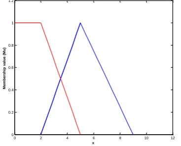
for any collection {Ai} in P(). Figure 1 (red line) represents the possibility of a fuzzy event characterized by x, where = (2,5,9) is a triangular fuzzy variable given by the mathematical form as
x
[image:3.595.80.274.101.317.2]
(5)
Fig. 1. Possibility that is greater than x It can be stated that the possibility of an event is determined by its most favourable case only, in contrast to the probability of an event, where all favourable cases are accumulated. By its very nature, the possibility measure is inconsistent with the law of excluded middle and the law of contradiction and does not satisfy the law of truth conservation.
Definition 2.6 Necessity Space
The necessity measure of a set A often is defined as the impossibility of the opposite set Ac [6]. Formally, let (, P(),Pos) be a possibility space, and A is a set in P(). Then the necessity measure of A is defined by
Nec{A} = 1 – Pos{Ac} (6)
Considering the triangular fuzzy variable = (2,5,9), we can represent Nec{ x} by eq.(7) (The red line of Fig. 2 shows the necessity measure),
(7)
It can be noted from Fig. 2 that, Nec{ x}= 1- Pos{ x}.
Fig. 2. Necessity that is greater than or equal to x
Definition 2.7 Credibility Space
Given the limitations of the possibility measure, Liu and Liu (2002) suggested replacing it with what they termed as credibility measure [7]. The credibility measure takes the form
Cr{X r} = 0.5 (Pos{ X r} + Nec{ X r}) (8)
or, equivalently,
sup
(
)
1
sup
(
)
2
1
}
{
X
r
t
t
Cr
tr
x
tr
xThe set {Cr} on the power set P is called a credibility measure if it satisfies the following four axioms [8]
(1) Normality: Cr{} = 1 (2) Monotonicity: Cr{A} Cr{B} whenever A B
(3) Self-Duality: Cr{A} + Cr{Ac} = 1 for any event A (4) Maximality: Cr{I Ai} = supi Cr{Ai} for any events
{Ai} with supi Cr{Ai} < 0.5
The triplet (, P(), Cr) is called a credibility space. It can be stated that the credibility measure is a special type of non-additive measure with self-duality. In this context, a fuzzy event may fail even though its possibility achieves 1, and may hold even though its necessity is 0. However, the fuzzy event must hold if its credibility is 1 and fail if its credibility is 0. The mathematical representation of the credibility of x can be written with the help of the given triangular fuzzy number (a, b, c) (2,5,9) as
x
(9)
[image:3.595.338.506.519.657.2]The solid red line as shown in Fig. 3 represents the credibility value of the fuzzy event characterized by x.
Fig.3. Credibility that is greater than or equal to x
Concepts of fuzzy number and α-cuts can be found elsewhere in [9] and for that reason let us define Borel sets:
Definition 2.8 Borel Sets
If F is a collection of subsets of the sample space, , then F is said to be a -algebra if the
following conditions hold: F;
0 1 2 3 4 5 6 7 8 9 10 0
0.2 0.4 0.6 0.8 1
x
mu
0 2 4 6 8 10 12
0 0.2 0.4 0.6 0.8 1 1.2
x
M
e
m
be
rs
hi
p
v
a
lue
(
M
u)
0 1 2 3 4 5 6 7 8 9 10 11 0
0.2 0.4 0.6 0.8 1 1.2
x
M
e
m
be
rs
hi
p
v
a
lue
(
M
[image:3.595.77.261.615.763.2]
1
i
A
i and Ai F for i I+, then A F. The Borel -algebra, B is the smallest -algebra that contains the set of all open intervals in R, the set of real numbers. Elements of B are called Borel sets and (R, B) is called Borel measurable space. An example can be given to clear the concept of Borel set. Let us consider the conflict case of consumption of wheat in a typical family in southern region of India. One group gave this figure as [100, 200] kg/yr and the other group said [150, 300] kg/yr. If at least one of these groups is correct, the consumption of wheat will fall within the union of two, i.e., [100,300]. But, if both the groups are correct, the consumption of wheat will fall in the intersection of their estimates, that is, the interval [150, 200]. Borel sets are used to describe these types of data.3. Fuzziness and Randomness – Are they same?
In order to implement the concept of fuzzy random variable for assessing the uncertainty of any physical model, it is mandatory to know whether randomness and fuzziness are connotation or not. It has been already pointed out in section 1 that these two are complementary, so, fuzziness and randomness are not the same. Basically randomness to fuzziness is one kind of paradigm shift. Randomness addresses the variability of the uncertain variable whereas fuzziness describes the ignorance of the variable. Fuzziness can be reduced whereas randomness can’t be reduced. Randomness is described by the probability distribution, whereas, fuzziness is represented by possibility distribution. Therefore, it can be envisaged that there exists a distributional difference as well as membership difference between fuzziness and randomness. Let us first focus on the distributional differences and demonstrate it by a simple example. A representative probability distribution, based on survey of radiation history of occupational workers in any nuclear plant, a probability of 0.94 can be assigned as zero overexposure, a 0.06 probability of one overexposure, and a 0.004 probability of two overexposures. In contrast, one can imagine that the representative possibility distribution of zero and one overexposure of occupational workers each has a high possibility of occurrence, and there is some possibility that the more than two occupational workers will be overexposed. Therefore, it can be concluded that, a probable event is always possible, while a possible event need not be probable. Zadeh (1978) called this heuristic connection between possibilities and probabilities the probability/possibility consistency principle [5]. This informal principle may be translated as: the degree of possibility of an event is greater than or equal to its degree of probability, which must be itself greater than or equal to its degree of necessity. Now consider the membership differences by accounting two groups of members of the public, one is within 5 km and the other is beyond 5 km of the site boundary of a radiochemical facility, and they are being classified as high dose and low dose category on the basis of the ingestion dose received. Ingestion dose received is due to the ingestion of contaminated food. There exists an uncertainty as to whether these groups are categorized perfectly or not in the sense that the dose received by the low dose category is very low and the dose received by the high category is moderately high. Low category is to be classified on the basis of ingestion dose received having
membership of 0.8 whereas high category is to be classified on the basis of probability and is known to have a probability of being a removal category of 0.9. Assuming one or other has to be classified as traditional ingestion dose, which one should be accepted for safety assessment. In this situation an obvious conclusion is that fuzzy degrees are not the same as probability percentages. That is, grade of membership is different from probability of membership.
4.0 Fuzzy Random Models
Three kind of fuzzy random variables such as (1) Kwakernaak model (here “fuzzy random variable” is interpreted as “random variables whose values are not real but fuzzy numbers”), (2) Puri and Ralescu model and (3) Liu and Liu model are cited in the literature [10-12]. Accordingly, we have three kinds of fuzzy random variable models and we present all the FRV models as follows:
4.2.1 Kwakernaak FRV Model
In this model, a FRV is a mapping : F(R) such that for any [0,1] and all , the real valued mapping is as follows:
,
:
inf
R
satisfying
inf
(
)
inf(
(
))
, and,
:
sup
R
satisfying
sup
(
)
sup(
(
))
. These real valued mappings are real valued random variables, that is, Borel-measurable real-valued functions. These -level constraints on may be summarized as].
))
(
sup(
,
))
(
[inf(
)
(
In short, the Kwakernaak FRV takes the form of a mapping from to the left and right hand side of the fuzzy target F(R), where the latter are real-valued random variables. If X
be a FRV and
Ais the collection of all A-measurable random variables of , then the kth moment of Kwakernaak FRV x, E(xk) is a fuzzy set on R withR
x
x
U
U
U
x
k A
x k
x E
},
,
|
)
(
sup{
)
(
) (
The fuzzy variance of X is a fuzzy set Vark(x) on [0,) with
)
,
0
[
},
,
|
)
(
sup{
)
(
2 2 2
2 ) ( var
U
D
U
U
A
x x
k
4.2.2 Puri and Ralescu FRV Model
Prior to present Puri and Ralescu (1986) FRV model [12], it is required to describe Banach space in short. Banach space is a normed linear space which is complete as a metric space. Banach spaces are used to extend the domain of FRVs from the real line to Euclidean n-space. Puri and Ralescu (1986) conceptualized a FRV as a fuzzification of a random set [12]. If (B, |.|) be a separable Banach space, K(B) be a nonempty compact subset of B, this model is addressed a FRV as a mapping : F(B) such that
() = (()) for all ) is a compact random set, that is, it is Borel-measurable with the Borel -field generated by the topology associated with the Hausdorff metric on K(B) [12] |} | inf sup |, | inf sup max{ ) , ( q p q p Q P d Q q P p H
q Q p P
If P and Q are bounded, then the Hausdorff metric becomes
|}
sup
sup
|
|,
inf
inf
max{|
)
,
(
q
p
q
p
Q
P
d
H
4.2.2.1 Expected value of a Puri and Ralescu FRV
It is known that a FRV is said to be an integrably bounded FRV associated with the probability space (, A, P) if an
only if
(
,
,
),
1
0
L
A
P
where, for the function f,
}
,
,
:
|
{
)
,
,
(
1 1
f
dP
measurable
A
R
f
f
P
A
L
Now, given the probability space (, A, P), an integrably bounded FRV associated with (, A, P), and S(F) a nonempty bounded set with respect to the L1(P)-norm, the
expected value of is the unique fuzzy set
(
|
)
~
P
E
of Rn such thatdP
P
E
|
))
(
~
(
for all [0,1],
where
)}
(
|
{
dP
f
dP
f
S
is the Aumann
integral [13] of with respect to P. Puri and Ralescu defined the expected value (EV) of a FRV as a generalization of the EV. Operationally, when a fuzzy random variable : F(R) is integrably bounded, the EV of is unique and for all [0,1], is given by the compact interval [E(inf ), E(sup )].
4.2.2.2 Variance of a Puri and Ralescu FRV
The variance should be used to measure the spread or dispersion of the FRV around its EV [14]. Accordingly, scalar variance of a Puri and Ralescu FRV is defined as
V
X
d
X
V
X
V
[
(
)
(
)]
2
1
)
(
1 0
4.3 The Liu and Liu FRV Model
Liu and Liu(2002, 2003) expressed concern that both the Kwakernaak and Puri and Ralescu FRV models were based on the possibility measure [15], and, as such, did not obey the law of truth conversation and were inconsistent with the law of excluded middle and the law of contradiction [15]. To overcome these perceived shortcomings, they based their FRV on the credibility measure [16], Cr{A} = 0.5(Pos{A} + 1 – Pos{Ac}), which they contended plays the role of probability measure more appropriately than either the possibility and necessity measures. Finally, their FRV model incorporated a scalar, rather than a fuzzy, expected value, since they viewed the latter as problematic from an implementation perspective. On the basis of credibility measure, Liu (2006) defines a fuzzy random variable as a
function from a probability space (, A, Pr) to the set of fuzzy variables such that Cr{()B} is a measurable function of for any Borel set B of R [16].
4.3.1 Expected value of the Liu and Liu FRV
If is fuzzy random variable defined on the probability space (, A, Pr), then the expected value of as per Liu and Liu (2006) is defined as [16-18]
0 0}
{
}
{
]
[
Cr
x
dx
Cr
x
dx
E
provided that at least one of the two integrals is finite. Alternatively, an expected value of can be conceptualized as
)
Pr(
]
}
)
(
{
}
)
(
{
[
]
[
0 0
d
dr
r
Cr
dr
r
Cr
E
provided that at least one of the two integrals is finite and in the event that is a nonnegative fuzzy random variable, expectation of [18] can be written as
0)
Pr(
}
)
(
{
]
[
Cr
r
dr
d
E
According to the definition of the expected value of fuzzy variable, , the equipossible fuzzy variable on [a, b] has an expected value (a + b)/2. The triangular fuzzy variable (a, b, c) has an expected value (a + 2b+ c)/4; this can be derived as follows:
dx
a
b
a
x
dx
c
b
c
x
b
E
b a c b
2
1
2
1
]
[
=
4
2
4
4
c
b
a
b
a
b
c
b
In a similar way, the trapezoidal fuzzy variable (a, b, c, d) has an expected value of (a + b + c + d)/4. As an example, a fuzzy variable, is called exponentially distributed if it has an exponential membership function
0
,
0
,
6
exp
1
2
)
(
1
m
x
m
x
x
; where, m is the parameter of the exponential membership function;
The expected value of the FRV, is
6
m
ln
2
. Further, if is a normal fuzzy variable with normal membership function [18]0
,
,
))
6
exp(
1
(
2
)
(
1
x
x
e
x
R
then, the expected value of is e.
4.3.2 Variance of the Liu and Liu FRV
If is a FRV with finite expected
defined as the expected value of the FRV ( - E[])2.
Therefore, we can write [18]
Var[] = E[( - E[] )2]
If is the fuzzy normal variable [18], then the variance of is
2 1
)
6
exp(
1
(
]
[
r
dr
Var
e5.0 Case Study – Radon Transport Model
Radon transport model in the fuzzy random form can be written as
(10)
where, the radon concentration,
C
~
is signifying as a fuzzy random number due to obvious reason. The tilde (‘~’) sign notifies the variable as fuzzy random variable. Numerical solution of this fuzzy random partial differential equation is obtained by first removing its fuzziness and randomness by the alpha cut value of the associated fuzzy random numbers,
D
~
, andv
~
. The details about a fuzzy set can be found elsewhere in [15].5.1 Formulation of Finite difference radon transport equation
In this work, the explicit forward time and central space (FTCS) finite difference scheme of the governing equation with alpha cut representation of the fuzzy random parameters
(diffusion coefficient
D
~
and flow velocityv
~
) at any percentile value of their randomness has been used. Fuzzy random representation of governing eq. (10) can be written as
(11)
Forward time and central space (FTCS) scheme are used for discretization of the time derivative and space derivative
terms (
)
~
~
,
~
2 2
x
C
and
x
C
t
C
. Since alpha cut representation of the fuzzy parameters are represented as bounded closed interval and positive definite, explicit finite difference scheme used on the alpha cut representation of the radon concentration for its lower and upper bound can be written as
C
Gk
h
k
v
h
k
D
C
h
k
D
k
C
h
k
v
h
k
D
C
iLj L L iL j L iLj L L iL j
2 1, 2 , 2 1,
1 ,
2
1
(12)
C
Gk
h
k
v
h
k
D
C
h
k
D
k
C
h
k
v
h
k
D
C
iUj U U iU j U iUj U U Ui j
2 1, 2 , 2 1,
1 ,
2
1
(13)
where indices i and j refer to the discrete step lengths h = x and k = t for the coordinate x and time t, respectively. The lower and upper bounds of all the fuzzy parameters at its any
-cut representation can be written as
[
D
L,
D
U]
, and respectively. Equation (12) and (13) represent formulae for lower and upper bounds of the radon concentration at the (i, j+1)th mesh points for any -cut in terms of known values along the (i-1)th, (i)th , (i+1)th distances and at jth time. In this way, the truncation error for the difference Eq. (12) and Eq. (13) are reduced to O (k, h2). Using a small enough value of k and h, the truncation error can be reduced until the accuracy achieved is within the error tolerance [16]. The finite difference forms of the initial condition for lower and upper bound of the radon concentration are given by,
0
Lo i
C
and ,
0
Uo i
C
for t = 0; 0 < x < L (14) The finite difference forms of the boundary conditions for lower and upper bound of the radon concentration are given by
C
0,C
0,C
0 Uj L
j
for x = 0; t> 0, (15)
,
,
0
Uj N L
j
N
C
C
for x = L; t > 0 (16)
where N = L/h is the grid dimension in the x direction. L is the total length of the soil slab considered for the computation.
5.2 Computation
Input Data:
Monte Carlo simulation technique is used to generate the sample values of random part of the FRV whereas alpha cut method is used to generate the compact interval of the fuzziness part of FRV. Computational scheme followed to generate the sample values of these FRVs are as follows:
a) The radon diffusion coefficient
)
],
,
,
([
~
~
r m l
N
D
is used as a fuzzy normal random variable, the mean of which is a triangular fuzzy variable and standard deviation is the 20% of the most likely value of the triangular fuzzy number.
The value of D is: {[2.4E-6, 4.0E-6, 5.6E-6], 8.0E-7} To generate sample values of FRV diffusion
coefficient, procedure is as follows:
Alpha cut representation of is first generated for each varying from 0 to 1 with an increment of 0.1. Each such alpha cut values of is a compact interval such as [LB, UB]. Now
D are generated by traditional sampling techniques of a normal distribution, lower bound with N(LB, ) and the other one with N(UB, ).
b)
= U([1.0E-7,
1.0E-6, 1.0E-5], [1.0E-6, 1.0E-5.1.0E-4]) is represented by uniform probability distribution, where lower and upper bounds of uniform distribution are a triangular fuzzy number.
To generate sample values of fuzzy random parameter :
Alpha cut representation of the lower and upper limits of the uniform distribution (both are triangular fuzzy number) of are constructed for each [0,1] with an increment of 0.1. So, here we have the structure as ~ U([LB1, UB1], [LB2, UB2]. All these bound values being positive number, sample values of the lower and upper bound of n are generated by traditional Monte Carlo sampling of an uniform distribution with U([LB1, LB2] and with U[UB1, UB2] respectively.
Output:
Generated values of radon concentration C as fuzzy random output.
The lower and upper bounds of fuzzy random distribution of the radon concentration, C are generated by using these sample values. Cumulative distribution of the randomness of two parameters at any alpha cut are used to obtain 5th and 95th percentiles as bounds of fuzziness of two FRVs. Numerical solution of radon concentrations at the end point of total simulation time (50000 s) for various spatial distances are generated by these intervals. The lower and upper bounds of concentration is populated with all the alpha cuts (i.e., = 0 to 1 with a step size of 0.1) as columns and sample size of the random distributions as rows. Sample size of 1000 values of each of the FRV were generated.
References
1. Rowe, R.K. and Booker, J.R., 1985. 1-D pollutant migration in soils of finite depth. ASCE Journal of Geotechnical engineering, 111 (4), 479-499.
2. Sharma, H.D. and Lewis, S.P., 1994. Waste containment systems, waste stabilisation and landfills: design and evaluation. Wiley, New York. 3. Bedient, P.N., Rifai, H.S., Newell, J.C., 1994. Ground water
contamination transport and remediation. Prentice Hall, Englewood Cliffs, NJ.
4. Gonazalez-Rodriguez, G., Coulbi, A., Gil, M.A., 2006. A fuzzy representation of random variables: An operational tool in exploratory analysis and hypothesis testing, Intl. J. of Computational Statistical Data Analysis, 51, 163-176.
5. Zadeh, L.A., 1968. Probability measures of fuzzy events, Journal of Mathematical Analysis and Applications, 23, 421-427.
6. Dubois, D., and Prade, J., 1980. Fuzzy Sets and Systems: Theory and Applications. In: Mathematics in Science and Engineering, 144, Academic Press, New York.
7. Liu, B., and Liu, Y. K., 2002. Expected value of fuzzy variable and fuzzy expected value models, IEEE Transaction on Fuzzy Systems, vol. 10, pp. 445-450.
8. Liu, B., 2005. Foundations of Uncertainty Theory, Department of Mathematical Sciences, Tsinghua University.
9. Klir, G. J., and Yuan, B., 1995. Fuzzy sets and Fuzzy Logic: Theory and Applications, Prentice Hall, PTR, Upper Saddle River, NJ.
10.Kwakernaak, H., 1978. Fuzzy random variables – I. definitions and theorems, Information Sciences, 15(1), 1-29.
11. Kwakernaak, H., 1979. Fuzzy random variables – II. Algorithms and examples for the discreet case, Information Sciences, 17(3), 253-278. 12. Puri, M.L., Ralescu, D.A., 1986. Fuzzy random variables, Journal of
Mathematical Analysis and Applications, 114, 409-422.
13. Anuman, R.J., 1965. Integrals of set-valued functions, J. Math. Anal. Appl., 12, 1-12.
14. Feng, Y., Hu, L. And Shu, H., 2001. The Variance and Covariance of Fuzzy Random Variables and their Applications, Fuzzy Sets and Systems, 120, 487-497.
15. Liu, Y.K. and Liu, B., 2003. Fuzzy Random Variables: A Scalar Expected Value Operator, Fuzzy Optimization and Decision Making, 2(2), 143-160.
16. Liu, B., 2006. A survey of credibility theory, Fuzzy Optimization and Decision Making, 5(4), 387-408.
17. Moller, B. And Beer, M., 2004. Fuzzy Randomness: Uncertainty in Civil Engineering and Computational Mechanics, Springer, Berlin Heidelberg, New York.
18. Liu, B., 2007, Uncertainty Theory, 2nd ed., Springer-Verlag, Berlin. 19. Shackelford, C.D., 1993. In: Daniel, D.E. (Ed.). Geotechnical practice
for waste disposal. Chapman & Hall, London.
20. Watts, R.J., 1998. Hazardous waste: sources, pathways, receptors. Wiley, New York.
AUTHORSPROFILE
Debabrata Datta ,Radiological Physics & Advisory Division ,Bhabha Atomic Research Centre ,Mumbai – [email protected]
Shakeela Sathish*,Department of Mathematics